

CORDEX Climate projections: evaluating bias in precipitation-based indices for impact models#
Use case: Verification of precipitation indices used as proxies for rainfall erosivity in Europe under future climate scenarios.#
Quality assessment question#
How well do CORDEX projections represent climatology and trends of precipitation-based indices in Europe?
Production date: 29-05-2024
Produced by: CMCC foundation - Euro-Mediterranean Center on Climate Change. Albert Martinez Boti.
Soil erosion stands as one of the primary environmental concerns in Europe [1]. Its accelerated occurrence can precipitate a decline in ecosystem stability, land productivity, and overall land degradation, resulting in diminished income for farmers [2]. This notebook is designed to evaluate the effectiveness of a specific set of models from CORDEX Regional Climate Models (RCMs) in accurately replicating historical precipitation extreme indices. These selected rainfall indicators are recognised as valuable proxies for rainfall erosivity, a factor directly linked to empirical calculations of soil loss, as outlined in an application available through the CDS platform (CDS). The five precipitation-based indices used here are calculated using the icclim package, them being:
Spell length of days with precipitation greater than 1 mm (also known as “Maximum consecutive wet days” - “CWD”)
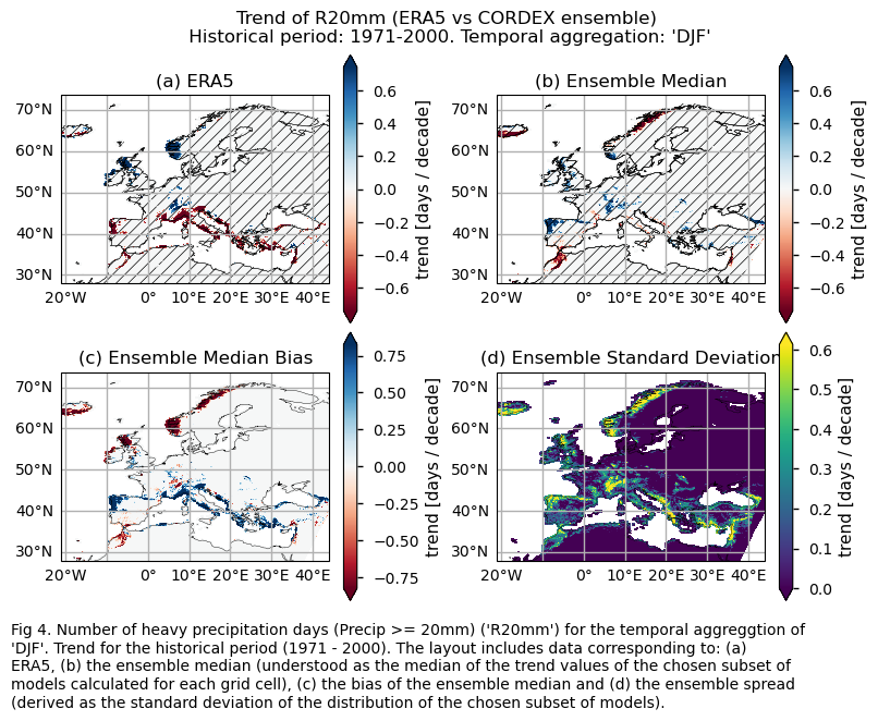
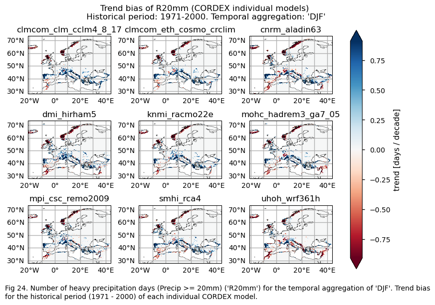
Number of heavy precipitation days (Precip >= 20mm - “R20mm”)
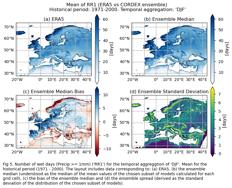
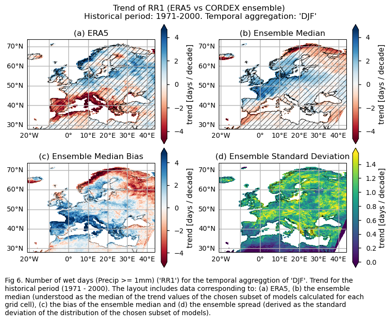
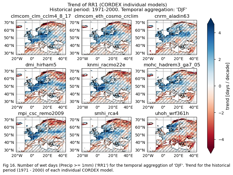
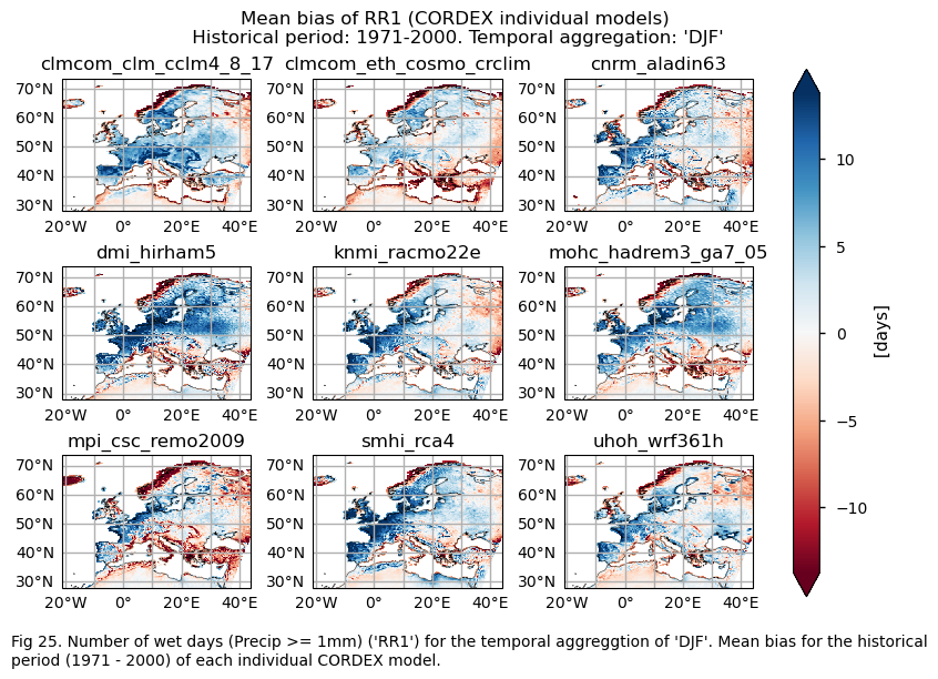
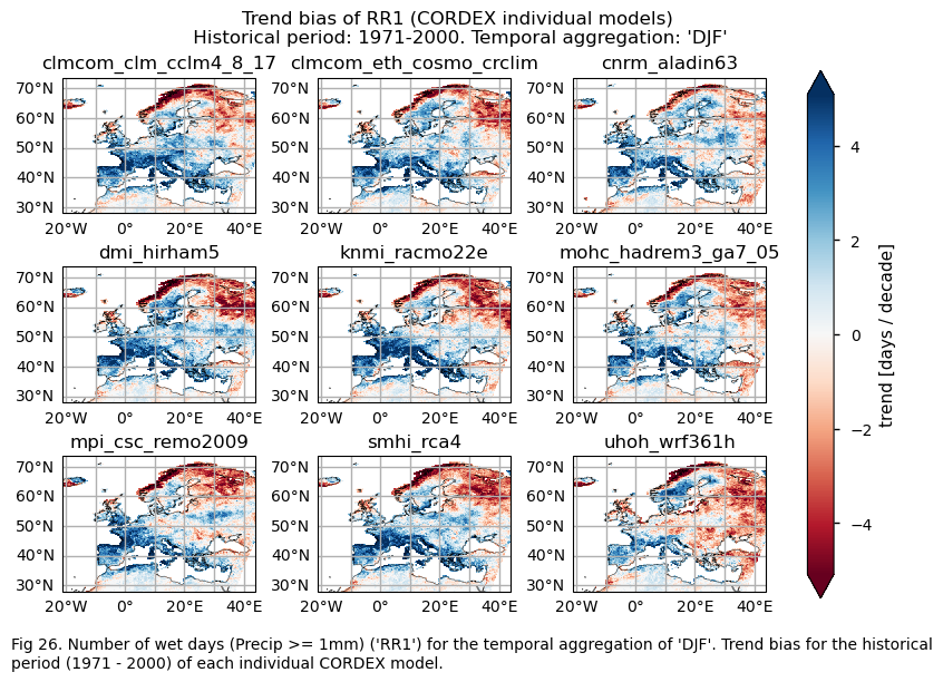
Number of wet days (Precip >= 1mm - “RR1”)
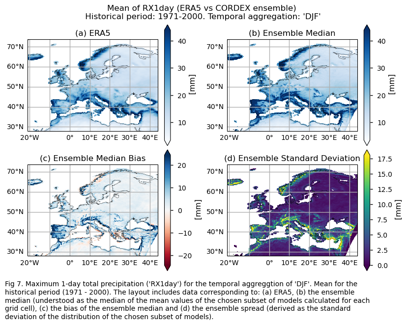
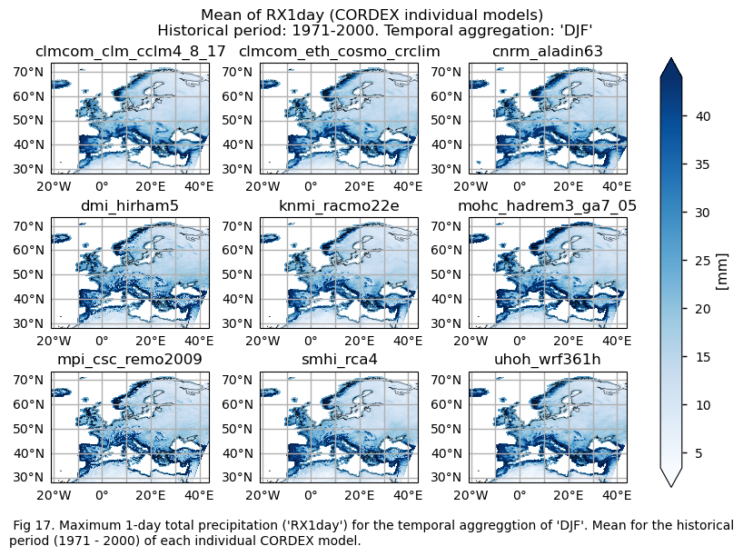
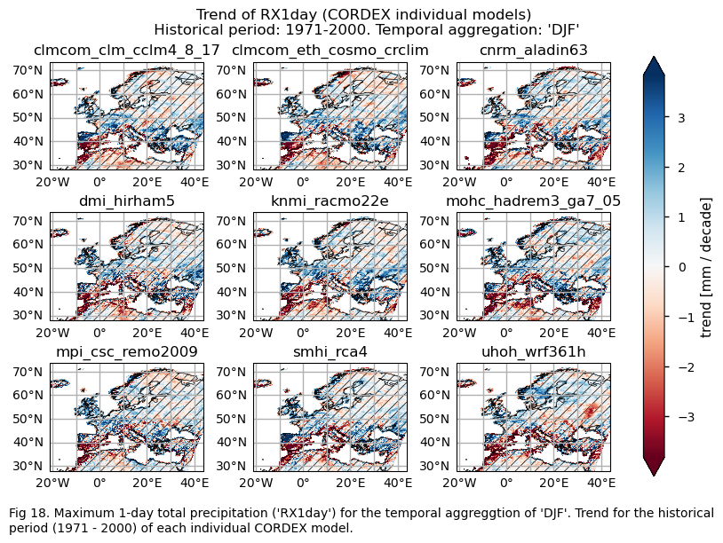
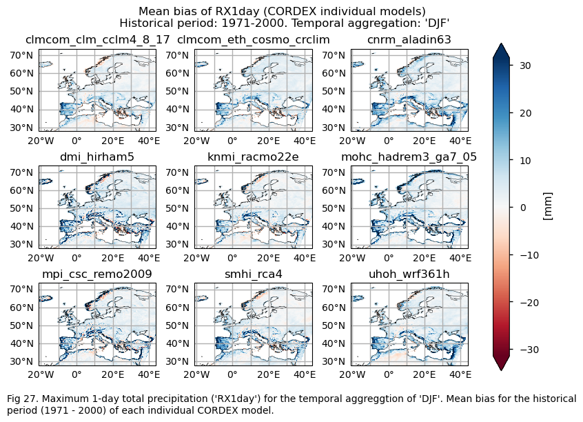
Maximum 1-day total precipitation (“RX1day”)
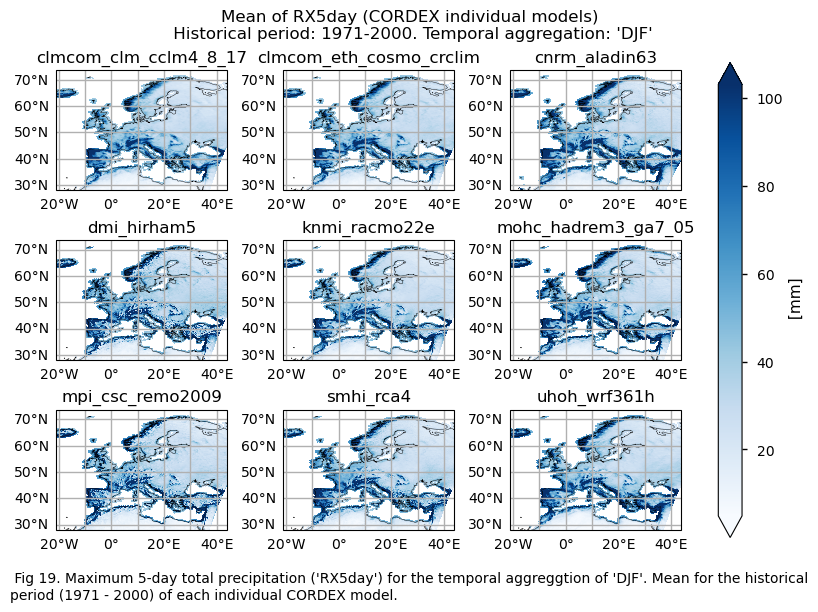
Maximum 5-day total precipitation (“RX5day”).
Within this notebook, these calculations are performed over the temporal aggregation of DJF and for the historical period spanning from 1971 to 2000. It is important to note that the results presented here pertain to a specific subset of the CORDEX ensemble and may not be generalisable to the entire dataset. Also note that a separate assessment examines the representation of trends of these indices for the same models during a fixed future period (2015-2099).
Quality assessment statement#
The assessment of CORDEX projections regarding the climatology and trend of precipitation-based indices across Europe requires a comprehensive evaluation of the historical period.
The subset of Regional Climate Models (RCMs) considered in this notebook for the seasonal aggregation of DJF generally struggle to replicate both the observed climatology and historical trends of the selected precipitation-based indices, with particular difficulty in capturing the trends. However, the models manage to accurately capture the climatology and trend directions for certain regions and indices. For instance, the models reflect an increasing trend for the CWD index in the western part of the Iberian Peninsula and an upward trend for RR1 in central Europe. Users should take into account these regional variations, the specific indices they intend to use, the differing bias behaviours between climatology and trends, and the necessity of bias-correcting data before using it for hydrological applications [3].
Precipitation trends in observational and reanalysis datasets are generally less robust and more challenging to detect compared to temperature trends. This limitation is also evident in model simulations.
While ERA5 serves as a reference dataset in this notebook, it is important to recognise its inherent uncertainties. Although uncertainties exist for all variables, these biases are especially relevant for variables like surface wind or precipitation, as shown in [4] and [5]. This highlights the need for cautious interpretation, particularly in the context of precipitation extremes.
A larger GCM-RCM matrix should be considered when addressing specific cases to enhance the robustness of the analysis and account for uncertainties [6][7].
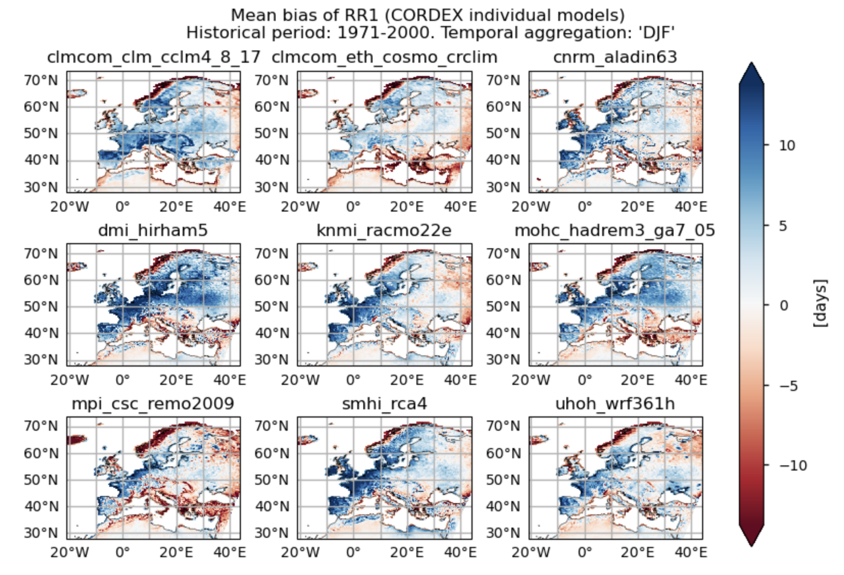
Fig A. Number of wet days (Precip >= 1mm) ('RRI') for the temporal aggreggtion of 'DJF'. Mean bias for the historical period (1971 - 2000) of each individual CORDEX model.
It is important to note that using seasonal temporal aggregations offers only partial insights into the dynamics. For more comprehensive results, it is advisable to also consider other seasons and annual aggregations. However, for the sake of efficiency and to avoid making the notebook too heavy, we have opted to prioritise seasonal aggregations.
Methodology#
This notebook provides an assessment of the systematic errors (trend and climatology) in a subset of 9 models from CORDEX. The analysis involves comparing model predictions with ERA5 reanalysis data using several precipitation-based indices. These indices, calculated over the DJF period for the historical period spanning from 1971 to 2000, include:
Spell length of days with precipitation greater than 1 mm (also known as “Maximum consecutive wet days” - “CWD”)
Number of heavy precipitation days (Precip >= 20mm - “R20mm”)
Number of wet days (Precip >= 1mm - “RR1”)
Maximum 1-day total precipitation (“RX1day”)
Maximum 5-day total precipitation (“RX5day”).
In particular, spatial patterns of climate mean and trend, along with biases, are examined and displayed for each model and the ensemble median (calculated for each grid cell). Additionally, spatially-averaged trend values are analysed and presented using box plots to provide an overview of trend behavior across the distribution of the chosen subset of models when averaged across Europe.
The analysis and results follow the next outline:
1. Parameters, requests and functions definition
Analysis and results#
1. Parameters, requests and functions definition#
1.1. Import packages#
Show code cell source
import math
import tempfile
import warnings
import textwrap
warnings.filterwarnings("ignore")

import cartopy.crs as ccrs
import icclim
import matplotlib.pyplot as plt
import xarray as xr
from c3s_eqc_automatic_quality_control import diagnostics, download, plot, utils
from xarrayMannKendall import Mann_Kendall_test

plt.style.use("seaborn-v0_8-notebook")
plt.rcParams["hatch.linewidth"] = 0.5
1.2. Define Parameters#
In the “Define Parameters” section, various customisable options for the notebook are specified:
The initial and ending year used for the historical period can be specified by changing the parameters
year_startandyear_stop(1971-2000 is chosen for consistency between CORDEX and CMIP6).The
timeseriesset the temporal aggregation. For instance, selecting “DJF” implies considering only the winter season.collection_idprovides the choice between Global Climate Models CMIP6 or Regional Climate Models CORDEX. Although the code allows choosing between CMIP6 or CORDEX, the example provided in this notebook deals with CORDEX RCMs.areaallows specifying the geographical domain of interest.The
interpolation_methodparameter allows selecting the interpolation method when regridding is performed over the indices.The
chunkselection allows the user to define if dividing into chunks when downloading the data on their local machine. Although it does not significantly affect the analysis, it is recommended to keep the default value for optimal performance.
Show code cell source
# Time period
year_start = 1971
year_stop = 2000
assert year_start >= 1971

# Choose annual or seasonal timeseries
timeseries = "DJF"
assert timeseries in ("annual", "DJF", "MAM", "JJA", "SON")

# Variable
variable = "precipitation"
assert variable in ("temperature", "precipitation")

# Choose CORDEX or CMIP6
collection_id = "CORDEX"
assert collection_id in ("CORDEX", "CMIP6")

# Interpolation method
interpolation_method = "bilinear"

# Area to show
area = [72, -22, 27, 45]

# Chunks for download
chunks = {"year": 1}
1.3. Define models#
The following climate analyses are performed considering a subset of GCMs from CMIP6. Models names are listed in the parameters below. Some variable-dependent parameters are also selected, as the index_names parameter, which specifies the precipitation-based indices (‘CWD’, ‘R20mm’, ‘RR1’, ‘RX1day’ and ‘RX5day’ in our case) from the icclim Python package.
When choosing Cordex models, it is crucial to consider the availability of RCMs for the selected GCM and the specified region. The listed RCMs, for instance, are accessible for the GCM “mpi_m_mpi_esm_lr” in the “europe” cordex_domain. To confirm the available combinations, refer to the CORDEX CDS catalogue entry.
Show code cell source
models_cordex = (
    "clmcom_clm_cclm4_8_17",
    "clmcom_eth_cosmo_crclim",
    "cnrm_aladin63",
    "dmi_hirham5",
    "knmi_racmo22e",
    "mohc_hadrem3_ga7_05",
    "mpi_csc_remo2009",
    "smhi_rca4",
    "uhoh_wrf361h",
)

match variable:
    case "temperature":
        resample_reduction = "max"
        index_names = ("SU", "TX90p")
        era5_variable = "2m_temperature"
        cordex_variable = "maximum_2m_temperature_in_the_last_24_hours"
        cmip6_variable = "daily_maximum_near_surface_air_temperature"
        models_cmip6 = (
            "access_cm2",
            "awi_cm_1_1_mr",
            "cmcc_esm2",
            "cnrm_cm6_1_hr",
            "ec_earth3_cc",
            "gfdl_esm4",
            "inm_cm5_0",
            "miroc6",
            "mpi_esm1_2_lr",
        )

        # Colormaps
        cmaps="viridis"
        cmaps_trend = cmaps_bias = "RdBu_r"
        #Define dictionaries to use in titles and caption
        long_name = {
            "SU":"Number of summer days",
            "TX90p":"Number of days with daily maximum temperatures exceeding the daily 90th percentile of maximum temperature for a 5-day moving window",
        }
    case "precipitation":
        resample_reduction = "sum"
        index_names = ("CWD", "R20mm", "RR1", "RX1day", "RX5day")
        era5_variable = "total_precipitation"
        cordex_variable = "mean_precipitation_flux"
        cmip6_variable = "precipitation"
        models_cmip6 = (
            "access_cm2",
            "bcc_csm2_mr",
            "cmcc_esm2",
            "cnrm_cm6_1_hr",
            "ec_earth3_cc",
            "gfdl_esm4",
            "inm_cm5_0",
            "miroc6",
            "mpi_esm1_2_lr",
        )
        # Colormaps
        cmaps="Blues"
        cmaps_trend = cmaps_bias = "RdBu"

        #Define dictionaries to use in titles and caption
        long_name = {
            "RX1day": "Maximum 1-day total precipitation",
            "RX5day": "Maximum 5-day total precipitation",
            "RR1":"Number of wet days (Precip >= 1mm)",
            "R20mm":"Number of heavy precipitation days (Precip >= 20mm)",
            "CWD":"Maximum consecutive wet days",
        }
    case _:
        raise NotImplementedError(f"{variable=}")
1.4. Define ERA5 request#
Within this notebook, ERA5 serves as the reference product. In this section, we set the required parameters for the cds-api data-request of ERA5.
Show code cell source
request_era = (
    "reanalysis-era5-single-levels",
    {
        "product_type": "reanalysis",
        "format": "netcdf",
        "time": [f"{hour:02d}:00" for hour in range(24)],
        "variable": era5_variable,
        "year": [
            str(year)
            for year in range(year_start - int(timeseries == "DJF"), year_stop + 1)
        ],  # Include D(year-1)
        "month": [f"{month:02d}" for month in range(1, 13)],
        "day": [f"{day:02d}" for day in range(1, 32)],
        "area": area,
    },
)

request_lsm = (
    request_era[0],
    request_era[1]
    | {
        "year": "1940",
        "month": "01",
        "day": "01",
        "time": "00:00",
        "variable": "land_sea_mask",
    },
)
1.5. Define model requests#
In this section we set the required parameters for the cds-api data-request.
The get_cordex_years function is employed to choose suitable data chunks for CORDEX data requests.
When Weights = True, spatial weighting is applied for calculations requiring spatial data aggregation. This is particularly relevant for CMIP6 GCMs with regular lon-lat grids that do not consider varying surface extensions at different latitudes. In contrast, CORDEX RCMs, using rotated grids, inherently account for different cell surfaces based on latitude, eliminating the need for a latitude cosine multiplicative factor (Weights = False).
Show code cell source
request_cordex = {
    "format": "zip",
    "domain": "europe",
    "experiment": "historical",
    "horizontal_resolution": "0_11_degree_x_0_11_degree",
    "temporal_resolution": "daily_mean",
    "variable": cordex_variable,
    "gcm_model": "mpi_m_mpi_esm_lr",
    "ensemble_member": "r1i1p1",
}

request_cmip6 = {
    "format": "zip",
    "temporal_resolution": "daily",
    "experiment": "historical",
    "variable": cmip6_variable,
    "year": [
        str(year) for year in range(year_start - 1, year_stop + 1)
    ],  # Include D(year-1)
    "month": [f"{month:02d}" for month in range(1, 13)],
    "day": [f"{day:02d}" for day in range(1, 32)],
    "area": area,
}


def get_cordex_years(
    year_start,
    year_stop,
    timeseries,
    start_years=list(range(1951, 2097, 5)),
    end_years=list(range(1955, 2101, 5)),
):
    start_year = []
    end_year = []
    years = set(range(year_start - int(timeseries == "DJF"), year_stop + 1))
    for start, end in zip(start_years, end_years):
        if years & set(range(start, end + 1)):
            start_year.append(start)
            end_year.append(end)
    return start_year, end_year


model_requests = {}
if collection_id == "CORDEX":
    for model in models_cordex:
        start_years = [1970 if model in ("smhi_rca4", "uhoh_wrf361h") else 1966] + list(
            range(1971, 2097, 5)
        )
        end_years = [1970] + list(range(1975, 2101, 5))
        model_requests[model] = (
            "projections-cordex-domains-single-levels",
            [
                {
                    "rcm_model": model,
                    **request_cordex,
                    "start_year": start_year,
                    "end_year": end_year,
                }
                for start_year, end_year in zip(
                    *get_cordex_years(
                        year_start,
                        year_stop,
                        timeseries,
                        start_years=start_years,
                        end_years=end_years,
                    )
                )
            ],
        )
elif collection_id == "CMIP6":
    for model in models_cmip6:
        model_requests[model] = (
            "projections-cmip6",
            download.split_request(request_cmip6 | {"model": model}, chunks=chunks),
        )
else:
    raise ValueError(f"{collection_id=}")
1.6. Functions to cache#
In this section, functions that will be executed in the caching phase are defined. Caching is the process of storing copies of files in a temporary storage location, so that they can be accessed more quickly. This process also checks if the user has already downloaded a file, avoiding redundant downloads.
Functions description:
The
select_timeseriesfunction subsets the dataset based on the chosentimeseriesparameter.The
compute_indicesfunction utilises the icclim package to calculate the precipitation-based indices.The
compute_trendsfunction employs the Mann-Kendall test for trend calculation.Finally, the
compute_indices_and_trendsaccumulates the daily precipitation (only if we are dealing with ERA5), calculates the precipitation-based indices for the corresponding temporal aggregation using thecompute_indicesfunction, determines the indices mean over the historical period (1971-2000), obtain the trends using thecompute_trendsfunction, and offers an option for regridding to ERA5 if required.
Show code cell source
def select_timeseries(ds, timeseries, year_start, year_stop, index_names):
    if timeseries == "annual":
        return ds.sel(time=slice(str(year_start), str(year_stop)))
    ds=ds.sel(time=slice(f"{year_start-1}-12", f"{year_stop}-11"))
    if "RX5day" in index_names:
        return ds
    return ds.where(ds["time"].dt.season == timeseries, drop=True)

def compute_indices(ds, index_names, timeseries, tmpdir):
    labels, datasets = zip(*ds.groupby("time.year"))
    paths = [f"{tmpdir}/{label}.nc" for label in labels]
    datasets = [ds.chunk(-1) for ds in datasets]
    xr.save_mfdataset(datasets, paths)

    ds = xr.open_mfdataset(paths)
    in_files = f"{tmpdir}/rechunked.zarr"
    chunks = {dim: 365 * 4 if dim == "time" else "auto" for dim in ds.dims}
    ds.chunk(chunks).to_zarr(in_files)

    datasets = [
        icclim.index(
            index_name=index_name,
            in_files=in_files,
            out_file=f"{tmpdir}/{index_name}.nc",
            slice_mode="year" if timeseries == "annual" else timeseries,
        )
        for index_name in index_names
    ]

    return xr.merge(datasets).drop_dims("bounds")


def compute_trends(ds):
    datasets = []
    (lat,) = set(ds.dims) & set(ds.cf.axes["Y"])
    (lon,) = set(ds.dims) & set(ds.cf.axes["X"])
    coords_name = {
        "time": "time",
        "y": lat,
        "x": lon,
    }
    for index, da in ds.data_vars.items():
        ds = Mann_Kendall_test(
            da - da.mean("time"),
            alpha=0.05,
            method="theilslopes",
            coords_name=coords_name,
        ).compute()
        ds = ds.rename({k: v for k, v in coords_name.items() if k in ds.dims})
        ds = ds.assign_coords({dim: da[dim] for dim in ds.dims})
        datasets.append(ds.expand_dims(index=[index]))
    ds = xr.concat(datasets, "index")
    return ds


def add_bounds(ds):
    for coord in {"latitude", "longitude"} - set(ds.cf.bounds):
        ds = ds.cf.add_bounds(coord)
    return ds


def get_grid_out(request_grid_out, method):
    ds_regrid = download.download_and_transform(*request_grid_out)
    coords = ["latitude", "longitude"]
    if method == "conservative":
        ds_regrid = add_bounds(ds_regrid)
        for coord in list(coords):
            coords.extend(ds_regrid.cf.bounds[coord])
    grid_out = ds_regrid[coords]
    coords_to_drop = set(grid_out.coords) - set(coords) - set(grid_out.dims)
    grid_out = ds_regrid[coords].reset_coords(coords_to_drop, drop=True)
    grid_out.attrs = {}
    return grid_out


def compute_indices_and_trends(
    ds,
    index_names,
    timeseries,
    year_start,
    year_stop,
    resample_reduction=None,
    request_grid_out=None,
    **regrid_kwargs,
):
    assert (request_grid_out and regrid_kwargs) or not (
        request_grid_out or regrid_kwargs
    )
    ds = ds.drop_vars([var for var, da in ds.data_vars.items() if len(da.dims) != 3])
    ds = ds[list(ds.data_vars)]

    # Original bounds for conservative interpolation
    if regrid_kwargs.get("method") == "conservative":
        ds = add_bounds(ds)
        bounds = [
            ds.cf.get_bounds(coord).reset_coords(drop=True)
            for coord in ("latitude", "longitude")
        ]
    else:
        bounds = []

    ds = select_timeseries(ds, timeseries, year_start, year_stop,index_names)
    if resample_reduction:
        resampled = ds.resample(time="1D")
        ds = getattr(resampled, resample_reduction)(keep_attrs=True)
        if resample_reduction == "sum":
            for da in ds.data_vars.values():
                da.attrs["units"] = f"{da.attrs['units']} / day"
    with tempfile.TemporaryDirectory() as tmpdir:
        ds_indices = compute_indices(ds, index_names, timeseries, tmpdir).compute()
        ds_trends = compute_trends(ds_indices)
        ds = ds_indices.mean("time", keep_attrs=True)
        ds = ds.merge(ds_trends)
        if request_grid_out:
            ds = diagnostics.regrid(
                ds.merge({da.name: da for da in bounds}),
                grid_out=get_grid_out(request_grid_out, regrid_kwargs["method"]),
                **regrid_kwargs,
            )
        return ds
2. Downloading and processing#
2.1. Download and transform ERA5#
In this section, the download.download_and_transform function from the ‘c3s_eqc_automatic_quality_control’ package is employed to download ERA5 reference data, accumulate daily precipitation from hourly data, compute the precipitation-based indices for the selected temporal aggregation (“DJF” in this example), calculate the mean and trend over the historical period (1971-2000) and cache the result (to avoid redundant downloads and processing).
Show code cell source
transform_func_kwargs = {
    "index_names": sorted(index_names),
    "timeseries": timeseries,
    "year_start": year_start,
    "year_stop": year_stop,
}
ds_era5 = download.download_and_transform(
    *request_era,
    chunks=chunks,
    transform_chunks=False,
    transform_func=compute_indices_and_trends,
    transform_func_kwargs=transform_func_kwargs
    | {"resample_reduction": resample_reduction},
)
2.2. Download and transform models#
In this section, the download.download_and_transform function from the ‘c3s_eqc_automatic_quality_control’ package is employed to download daily data from the CORDEX models, compute the precipitation-based indices for the selected temporal aggregation, calculate the mean and trend over the historical period (1971-2005), interpolate to ERA5’s grid (only for the cases in which it is specified, in the other cases, the original model’s grid is mantained), and cache the result (to avoid redundant downloads and processing).
Show code cell source
interpolated_datasets = []
model_datasets = {}
for model, requests in model_requests.items():
    print(f"{model=}")
    model_kwargs = {
        "chunks": chunks if collection_id == "CMIP6" else None,
        "transform_chunks": False,
        "transform_func": compute_indices_and_trends,
    }
    # Original model
    model_datasets[model] = download.download_and_transform(
        *requests,
        **model_kwargs,
        transform_func_kwargs=transform_func_kwargs,
    )

    # Interpolated model
    ds = download.download_and_transform(
        *requests,
        **model_kwargs,
        transform_func_kwargs=transform_func_kwargs
        | {
            "request_grid_out": request_lsm,
            "method": interpolation_method,
            "skipna": True,
        },
    )
    interpolated_datasets.append(ds.expand_dims(model=[model]))

ds_interpolated = xr.concat(interpolated_datasets, "model",coords='minimal',compat='override')
model='clmcom_clm_cclm4_8_17'
model='clmcom_eth_cosmo_crclim'
model='cnrm_aladin63'
model='dmi_hirham5'
model='knmi_racmo22e'
model='mohc_hadrem3_ga7_05'
model='mpi_csc_remo2009'
model='smhi_rca4'
model='uhoh_wrf361h'
2.3. Apply land-sea mask, change attributes and cut the region to show#
This section performs the following tasks:
Cut the region of interest.
Downloads the sea mask for ERA5.
Applies the sea mask to both ERA5 data and the model data, which were previously regridded to ERA5’s grid (i.e., it applies the ERA5 sea mask to
ds_interpolated).Regrids the ERA5 land-sea mask to the model’s grid and applies it to them.
Change some variable attributes for plotting purposes.
Note: ds_interpolated contains data from the models (mean and trend over the historical period, p-value of the trends…) regridded to ERA5. model_datasets contain the same data but in the original grid of each model.
Show code cell source
lsm = download.download_and_transform(*request_lsm)["lsm"].squeeze(drop=True)

# Cutout
regionalise_kwargs = {
    "lon_slice": slice(area[1], area[3]),
    "lat_slice": slice(area[0], area[2]),
}
lsm = utils.regionalise(lsm, **regionalise_kwargs)
ds_interpolated = utils.regionalise(ds_interpolated, **regionalise_kwargs)
model_datasets = {
    model: utils.regionalise(ds, **regionalise_kwargs)
    for model, ds in model_datasets.items()
}

# Mask
ds_era5 = ds_era5.where(lsm)
ds_interpolated = ds_interpolated.where(lsm)
model_datasets = {
    model: ds.where(diagnostics.regrid(lsm, ds, method="bilinear"))
    for model, ds in model_datasets.items()
}

# Edit attributes
for ds in (ds_era5, ds_interpolated, *model_datasets.values()):
    ds["trend"] *= 10
    ds["trend"].attrs = {"long_name": "trend"}
    for index in index_names:
        ds[index].attrs = {"long_name": "", "units": "days" if ds[index].attrs["units"]=="d"
                           else ("mm" if ds[index].attrs["units"]=="mm d-1"
                                 else ds[index].attrs["units"])}
3. Plot and describe results#
This section will display the following results:
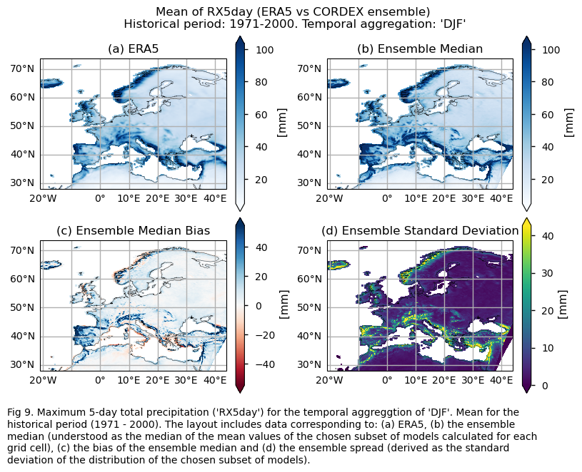
Maps representing the spatial distribution of the historical mean values (1971-2000) of the indices (‘CWD’, ‘R20mm’, ‘RR1’, ‘RX1day’ and ‘RX5day’) for ERA5, each model individually, the ensemble median (understood as the median of the mean values of the chosen subset of models calculated for each grid cell), and the ensemble spread (derived as the standard deviation of the distribution of the chosen subset of models).
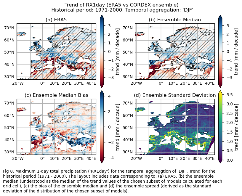
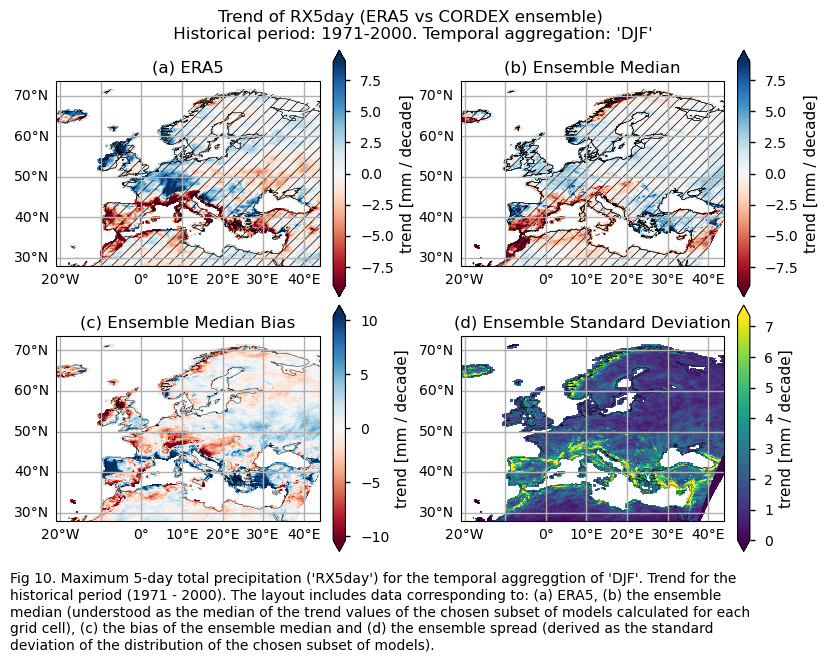
Maps representing the spatial distribution of the historical trends (1971-2000) of the considered indices. Similar to the first analysis, this includes ERA5, each model individually, the ensemble median (understood as the median of the trend values of the chosen subset of models calculated for each grid cell), and the ensemble spread (derived as the standard deviation of the distribution of the chosen subset of models).
Bias maps of the historical mean values.
Trend bias maps.
Boxplots representing statistical distributions (PDF) built on the spatially-averaged historical trends from each considered model, displayed together with ERA5.
3.1. Define plotting functions#
The functions presented here are used to plot the mean values and trends calculated over the historical period (1971-2000) for each of the indices (‘CWD’, ‘R20mm’, ‘RR1’, ‘RX1day’ and ‘RX5day’).
For a selected index, three layout types can be displayed, depending on the chosen function:
Layout including the reference ERA5 product, the ensemble median, the bias of the ensemble median, and the ensemble spread:
plot_ensemble()is used.Layout including every model (for the trend and mean values):
plot_models()is employed.Layout including the bias of every model (for the trend and mean values):
plot_models()is used again.
trend==True argument allows displaying trend values over the historical period, while trend==False will show mean values. When the trend argument is set to True, regions with no significance are hatched. For individual models and ERA5, a grid point is considered to have a statistically significant trend when the p-value is lower than 0.05 (in such cases, no hatching is shown). However, for determining trend significance for the ensemble median (understood as the median of the trend values of the chosen subset of models calculated for each grid cell), reliance is placed on agreement categories, following the advanced approach proposed in AR6 IPCC on pages 1945-1950. The hatch_p_value_ensemble() function is used to distinguish, for each grid point, between three possible cases:
If more than 66% of the models are statistically significant (p-value < 0.05) and more than 80% of the models share the same sign, we consider the ensemble median trend to be statistically significant, and there is agreement on the sign. To represent this, no hatching is used.
If less than 66% of the models are statistically significant, regardless of agreement on the sign of the trend, hatching is applied (indicating that the ensemble median trend is not statistically significant).
If more than 66% of the models are statistically significant but less than 80% of the models share the same sign, we consider the ensemble median trend to be statistically significant, but there is no agreement on the sign of the trend. This is represented using crosses.
Show code cell source
#Define function to plot the caption of the figures (for the ensmble case)
def add_caption_ensemble(trend,exp):
#Add caption to the figure
match trend:
case True:
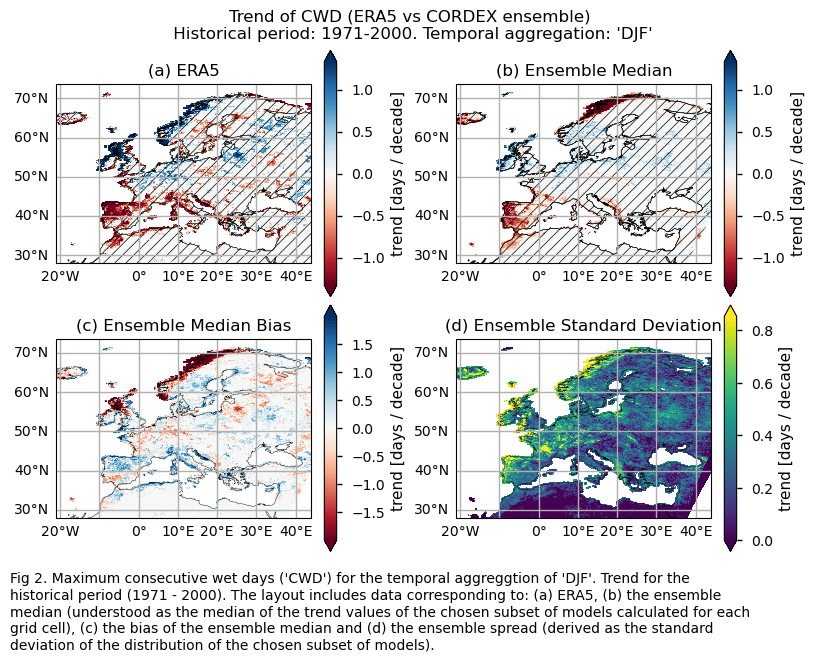
caption_text= (
f"Fig {fig_number}. {long_name[index]} ('{index}') for "
f"the temporal aggreggtion of '{timeseries}'. Trend for "
f"the {exp} period ({year_start} - {year_stop}). The layout "
f"includes data corresponding to: (a) ERA5, (b) the ensemble median "
f"(understood as the median of the trend values of the chosen subset of models "
f"calculated for each grid cell), "
f"(c) the bias of the ensemble median and (d) the ensemble spread "
f"(derived as the standard deviation of the distribution of the chosen "
f"subset of models)."
)
case False:
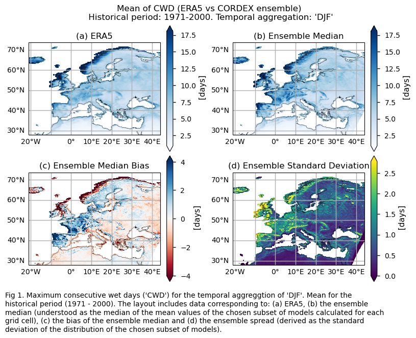
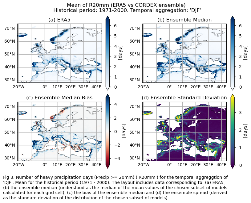
caption_text= (
f"Fig {fig_number}. {long_name[index]} ('{index}') for "
f"the temporal aggreggtion of '{timeseries}'. Mean for "
f"the {exp} period ({year_start} - {year_stop}). The layout "
f"includes data corresponding to: (a) ERA5, (b) the ensemble median "
f"(understood as the median of the mean values of the chosen subset of models "
f"calculated for each grid cell), "
f"(c) the bias of the ensemble median and (d) the ensemble spread "
f"(derived as the standard deviation of the distribution of the chosen "
f"subset of models)."
)
wrapped_lines = textwrap.wrap(caption_text, width=105)
# Add each line to the figure
for i, line in enumerate(wrapped_lines):
fig.text(0, -0.05 - i * 0.03, line, ha='left', fontsize=10)
#end captioning
#Define function to plot the caption of the figures (for the individual models case)
def add_caption_models(trend,bias,exp):
#Add caption to the figure
if bias:
match trend:
case True:
caption_text = (
f"Fig {fig_number}. {long_name[index]} ('{index}') for the "
f"temporal aggregation of '{timeseries}'. Trend bias for the "
f"{exp} period ({year_start} - {year_stop}) of each individual "
f"{collection_id} model."
)
case False:
caption_text = (
f"Fig {fig_number}. {long_name[index]} ('{index}') for the "
f"temporal aggreggtion of '{timeseries}'. Mean bias for the "
f"{exp} period ({year_start} - {year_stop}) of each individual "
f"{collection_id} model."
)
else:
match trend:
case True:
caption_text = (
f"Fig {fig_number}. {long_name[index]} ('{index}') for the "
f"temporal aggreggtion of '{timeseries}'. Trend for the {exp} "
f"period ({year_start} - {year_stop}) of each individual "
f"{collection_id} model."
)
case False:
caption_text = (
f" Fig {fig_number}. {long_name[index]} ('{index}') for the "
f"temporal aggreggtion of '{timeseries}'. Mean for the {exp} "
f"period ({year_start} - {year_stop}) of each individual "
f"{collection_id} model."
)
wrapped_lines = textwrap.wrap(caption_text, width=120)
# Add each line to the figure
for i, line in enumerate(wrapped_lines):
fig.text(0, -0.05 - i * 0.03, line, ha='left', fontsize=10)
def hatch_p_value(da, ax, **kwargs):
default_kwargs = {
"plot_func": "contourf",
"show_stats": False,
"cmap": "none",
"add_colorbar": False,
"levels": [0, 0.05, 1],
"hatches": ["", "/" * 3],
}
kwargs = default_kwargs | kwargs
title = ax.get_title()
plot_obj = plot.projected_map(da, ax=ax, **kwargs)
ax.set_title(title)
return plot_obj
def hatch_p_value_ensemble(trend, p_value, ax):
n_models = trend.sizes["model"]
robust_ratio = (p_value <= 0.05).sum("model") / n_models
robust_ratio = robust_ratio.where(p_value.notnull().any("model"))
signs = xr.concat([(trend > 0).sum("model"), (trend < 0).sum("model")], "sign")
sign_ratio = signs.max("sign") / n_models
robust_threshold = 0.66
sign_ratio = sign_ratio.where(robust_ratio > robust_threshold)
for da, threshold, character in zip(
[robust_ratio, sign_ratio], [robust_threshold, 0.8], ["/", "\\"]
):
hatch_p_value(da, ax=ax, levels=[0, threshold, 1], hatches=[character * 3, ""])
def set_extent(da, axs, area):
extent = [area[i] for i in (1, 3, 2, 0)]
for i, coord in enumerate(extent):
extent[i] += -1 if i % 2 else +1
for ax in axs:
ax.set_extent(extent)
def plot_models(
data,
da_for_kwargs=None,
p_values=None,
col_wrap=4 if collection_id=="CMIP6" else 3,
subplot_kw={"projection": ccrs.PlateCarree()},
figsize=None,
layout="constrained",
area=area,
**kwargs,
):
if isinstance(data, dict):
assert da_for_kwargs is not None
model_dataarrays = data
else:
da_for_kwargs = da_for_kwargs or data
model_dataarrays = dict(data.groupby("model"))
if p_values is not None:
model_p_dataarrays = (
p_values if isinstance(p_values, dict) else dict(p_values.groupby("model"))
)
else:
model_p_dataarrays = None
# Get kwargs
default_kwargs = {"robust": True, "extend": "both"}
kwargs = default_kwargs | kwargs
kwargs = xr.plot.utils._determine_cmap_params(da_for_kwargs.values, **kwargs)
fig, axs = plt.subplots(
*(col_wrap, math.ceil(len(model_dataarrays) / col_wrap)),
subplot_kw=subplot_kw,
figsize=figsize,
layout=layout,
)
axs = axs.flatten()
for (model, da), ax in zip(model_dataarrays.items(), axs):
pcm = plot.projected_map(
da, ax=ax, show_stats=False, add_colorbar=False, **kwargs
)
ax.set_title(model)
if model_p_dataarrays is not None:
hatch_p_value(model_p_dataarrays[model], ax)
set_extent(da_for_kwargs, axs, area)
fig.colorbar(
pcm,
ax=axs.flatten(),
extend=kwargs["extend"],
location="right",
label=f"{da_for_kwargs.attrs.get('long_name', '')} [{da_for_kwargs.attrs.get('units', '')}]",
)
return fig
def plot_ensemble(
da_models,
da_era5=None,
p_value_era5=None,
p_value_models=None,
subplot_kw={"projection": ccrs.PlateCarree()},
figsize=None,
layout="constrained",
cbar_kwargs=None,
area=area,
cmap_bias=None,
cmap_std=None,
**kwargs,
):
# Get kwargs
default_kwargs = {"robust": True, "extend": "both"}
kwargs = default_kwargs | kwargs
kwargs = xr.plot.utils._determine_cmap_params(
da_models.values if da_era5 is None else da_era5.values, **kwargs
)
if da_era5 is None and cbar_kwargs is None:
cbar_kwargs = {"orientation": "horizontal"}
# Figure
fig, axs = plt.subplots(
*(1 if da_era5 is None else 2, 2),
subplot_kw=subplot_kw,
figsize=figsize,
layout=layout,
)
axs = axs.flatten()
axs_iter = iter(axs)
# ERA5
if da_era5 is not None:
ax = next(axs_iter)
plot.projected_map(
da_era5, ax=ax, show_stats=False, cbar_kwargs=cbar_kwargs, **kwargs
)
if p_value_era5 is not None:
hatch_p_value(p_value_era5, ax=ax)
ax.set_title("(a) ERA5")
# Median
ax = next(axs_iter)
median = da_models.median("model", keep_attrs=True)
plot.projected_map(
median, ax=ax, show_stats=False, cbar_kwargs=cbar_kwargs, **kwargs
)
if p_value_models is not None:
hatch_p_value_ensemble(trend=da_models, p_value=p_value_models, ax=ax)
ax.set_title("(b) Ensemble Median" if da_era5 is not None else "(a) Ensemble Median")
# Bias
if da_era5 is not None:
ax = next(axs_iter)
with xr.set_options(keep_attrs=True):
bias = median - da_era5
plot.projected_map(
bias,
ax=ax,
show_stats=False,
center=0,
cbar_kwargs=cbar_kwargs,
**(default_kwargs | {"cmap": cmap_bias}),
)
ax.set_title("(c) Ensemble Median Bias")
# Std
ax = next(axs_iter)
std = da_models.std("model", keep_attrs=True)
plot.projected_map(
std,
ax=ax,
show_stats=False,
cbar_kwargs=cbar_kwargs,
**(default_kwargs | {"cmap": cmap_std}),
)
ax.set_title("(d) Ensemble Standard Deviation" if da_era5 is not None else "(b) Ensemble Standard Deviation")
set_extent(da_models, axs, area)
return fig
3.2. Plot ensemble maps#
In this section, we invoke the plot_ensemble() function to visualise the mean values and trends calculated over the historical period (1971-2000) for the model ensemble and ERA5 reference product across Europe. Note that the model data used in this section has previously been interpolated to the ERA5 grid.
Specifically, for each of the indices (‘CWD’, ‘R20mm’, ‘RR1’, ‘RX1day’ and ‘RX5day’), this section presents two layouts:
Mean values of the historical period (1971-2000) for: (a) the reference ERA5 product, (b) the ensemble median (understood as the median of the mean values of the chosen subset of models calculated for each grid cell), (c) the bias of the ensemble median, and (d) the ensemble spread (derived as the standard deviation of the distribution of the chosen subset of models).
Trend values of the historical period (1971-2000) for: (a) the reference ERA5 product, (b) the ensemble median (understood as the median of the trend values of the chosen subset of models calculated for each grid cell), (c) the bias of the ensemble median, and (d) the ensemble spread (derived as the standard deviation of the distribution of the chosen subset of models).
Show code cell source
#Fig number counter
fig_number=1

#Common title
common_title = f"Historical period: {year_start}-{year_stop}. Temporal aggregation: '{timeseries}'"

for index in index_names:
    # Index
    da = ds_interpolated[index]
    if (index!="TX90p"):
        fig = plot_ensemble(da_models=da,
                            da_era5=ds_era5[index],
                            cmap=cmaps,
                            cmap_bias=cmaps_bias)
        fig.suptitle(f"Mean of {index} (ERA5 vs {collection_id} ensemble)\n {common_title}")
        add_caption_ensemble(trend=False,exp="historical")
        plt.show()
        fig_number=fig_number+1
        print(f"\n")

    # Trend
    da_trend = ds_interpolated["trend"].sel(index=index)
    da_trend.attrs["units"] = f"{da.attrs['units']} / decade"
    da_era5= ds_era5["trend"].sel(index=index)
    da_era5.attrs["units"] = f"{da.attrs['units']} / decade"

    fig = plot_ensemble(
        da_models=da_trend,
        da_era5=da_era5,
        p_value_era5=ds_era5["p"].sel(index=index),
        p_value_models=ds_interpolated["p"].sel(index=index),
        center=0,
        cmap=cmaps_trend,
        cmap_bias=cmaps_bias,
    )
    fig.suptitle(f"Trend of {index} (ERA5 vs {collection_id} ensemble)\n {common_title}")
    add_caption_ensemble(trend=True,exp="historical")
    plt.show()
    fig_number=fig_number+1
    print(f"\n")
3.3. Plot model maps#
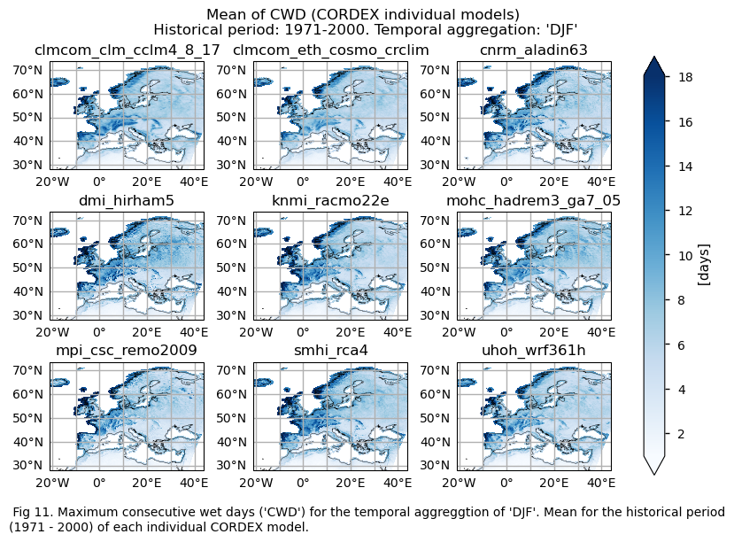
In this section, we invoke the plot_models() function to visualise the mean values and trends calculated over the historical period (1971-2000) for every model individually across Europe. Note that the model data used in this section maintains its original grid.
Specifically, for each of the indices (‘CWD’, ‘R20mm’, ‘RR1’, ‘RX1day’ and ‘RX5day’), this section presents two layouts:
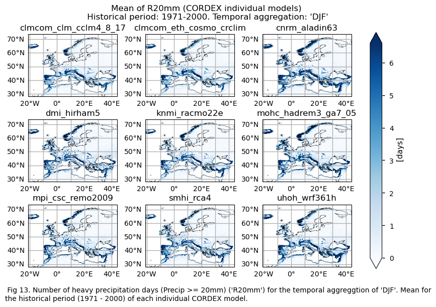
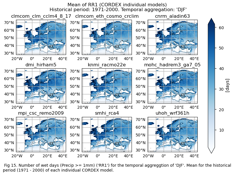
A layout including the historical mean (1971-2000) of every model (only for the ‘SU’ index).
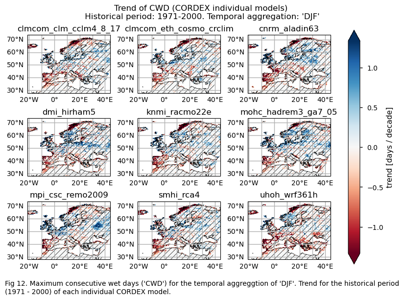
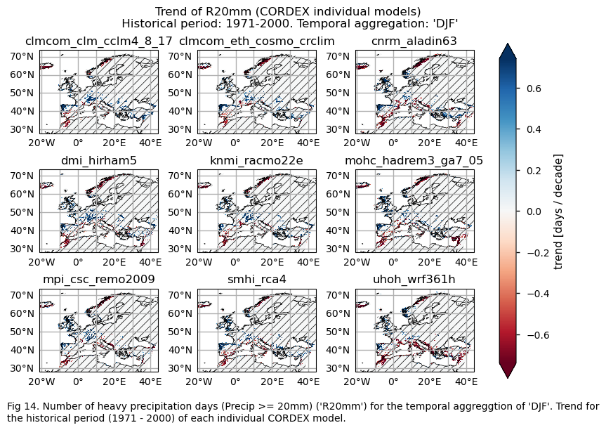
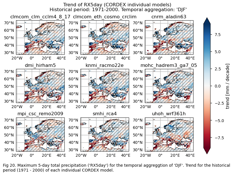
A layout including the historical trend (1971-2000) of every model.
Show code cell source
for index in index_names:
    # Index
    da_for_kwargs = ds_era5[index]
    if (index!="TX90p"):
        fig = plot_models(
            data={model: ds[index] for model, ds in model_datasets.items()},
            da_for_kwargs=da_for_kwargs,
            cmap=cmaps
        )
        fig.suptitle(f"Mean of {index} ({collection_id} individual models)\n {common_title}")
        add_caption_models(trend=False,bias=False,exp="historical")
        plt.show()
        print(f"\n")
        fig_number=fig_number+1

    # Trend
    da_for_kwargs_trends = ds_era5["trend"].sel(index=index)
    da_for_kwargs_trends.attrs["units"] = f"{da_for_kwargs.attrs['units']} / decade"
    fig = plot_models(
        data={
            model: ds["trend"].sel(index=index) for model, ds in model_datasets.items()
        },
        da_for_kwargs=da_for_kwargs_trends,
        p_values={
            model: ds["p"].sel(index=index) for model, ds in model_datasets.items()
        },
        center=0,
        cmap=cmaps_trend,
    )
    fig.suptitle(f"Trend of {index} ({collection_id} individual models)\n {common_title}")
    add_caption_models(trend=True,bias=False,exp="historical")
    plt.show()
    print(f"\n")
    fig_number=fig_number+1
3.4. Plot bias maps#
In this section, we invoke the plot_models() function to visualise the bias for the mean values and trends calculated over the historical period (1971-2000) for every model individually across Europe. Note that the model data used in this section has previously been interpolated to the ERA5 grid.
Specifically, for each of the indices (‘CWD’, ‘R20mm’, ‘RR1’, ‘RX1day’ and ‘RX5day’), this section presents two layouts:
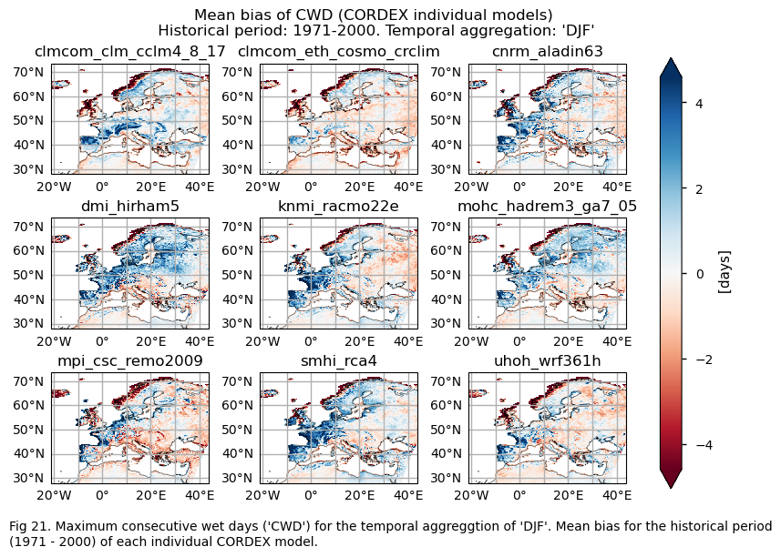
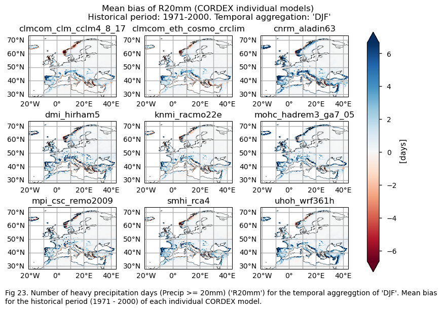
A layout including the bias for the historical mean (1971-2000) of every model (only for the ‘SU’ index).
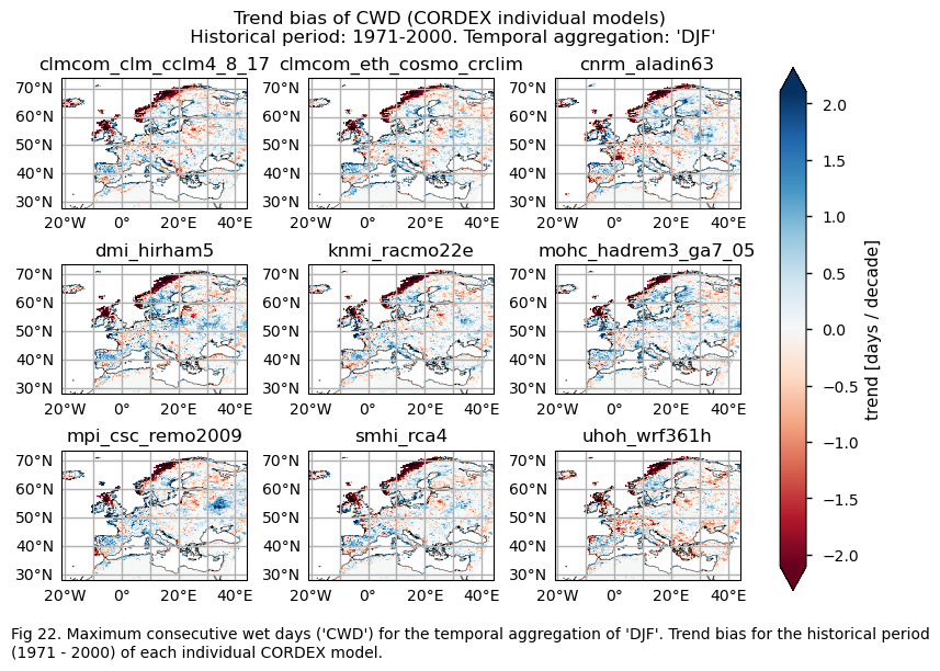
A layout including the bias for the historical trend (1971-2000) of every model.
Show code cell source
with xr.set_options(keep_attrs=True):
bias = ds_interpolated - ds_era5
for index in index_names:
# Index bias
da = bias[index]
if (index!="TX90p"):
fig = plot_models(data=da, center=0,cmap=cmaps_bias)
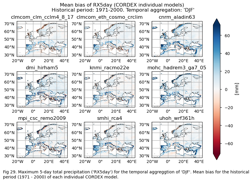
fig.suptitle(f"Mean bias of {index} ({collection_id} individual models)\n {common_title}")
add_caption_models(trend=False,bias=True,exp="historical")
plt.show()
print(f"\n")
fig_number=fig_number+1
# Trend bias
da_trend = bias["trend"].sel(index=index)
da_trend.attrs["units"] = f"{da.attrs['units']} / decade"
fig = plot_models(data=da_trend, center=0,cmap=cmaps_bias)
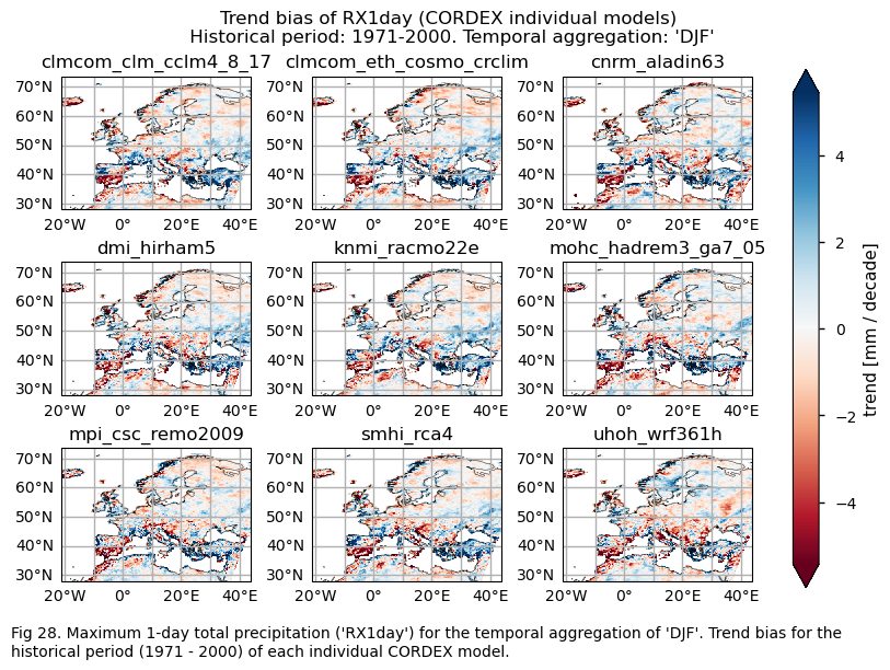
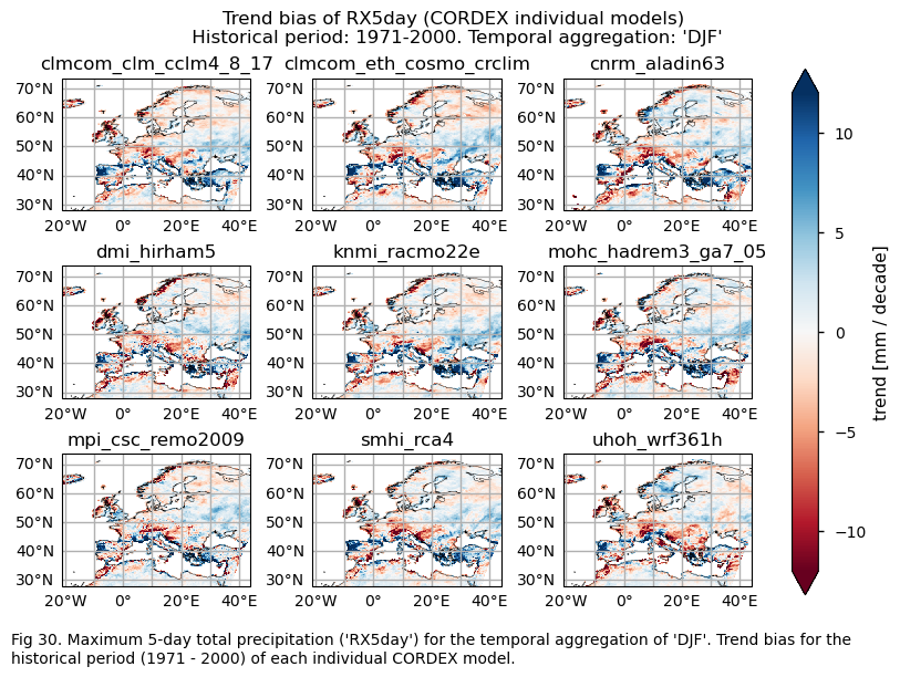
fig.suptitle(f"Trend bias of {index} ({collection_id} individual models)\n {common_title}")
add_caption_models(trend=True,bias=True,exp="historical")
plt.show()
print(f"\n")
fig_number=fig_number+1
plt.show()
3.5. Boxplots of the historical trend#
In this last section, we compare the trends of the climate models with the reference trend from ERA5.
Dots represent the spatially-averaged historical trend over the selected region (change of the number of days per decade) for each model (grey), the ensemble mean (blue), and the reference product (orange). The ensemble median is shown as a green line. Note that the spatially averaged values are calculated for each model from its original grid (i.e., no interpolated data has been used here).
The boxplot visually illustrates the distribution of trends among the climate models, with the box covering the first quartile (Q1 = 25th percentile) to the third quartile (Q3 = 75th percentile), and a green line indicating the ensemble median (Q2 = 50th percentile). Whiskers extend from the edges of the box to show the full data range.
Show code cell source
weights = collection_id == "CMIP6"
mean_datasets = [
    diagnostics.spatial_weighted_mean(ds.expand_dims(model=[model]), weights=weights)
    for model, ds in model_datasets.items()
]
mean_ds = xr.concat(mean_datasets, "model", coords='minimal',compat='override')
index_str=1

for index, da in mean_ds["trend"].groupby("index"):
    df_slope = da.to_dataframe()[["trend"]]
    ax = df_slope.boxplot()
    ax.scatter(
        x=[1] * len(df_slope),
        y=df_slope,
        color="grey",
        marker=".",
        label="models",
    )

    # Ensemble mean
    ax.scatter(
            x=1,
            y=da.mean("model"),
            marker="o",
            label=f"{collection_id} Ensemble Mean",
    )

    # ERA5
    labels = [f"{collection_id} Ensemble"]
    da = ds_era5["trend"].sel(index=index)
    da = diagnostics.spatial_weighted_mean(da)
    ax.scatter(
            x=2,
            y=da.values,
            marker="o",
            label="ERA5",
    )
    labels.append("ERA5")

    ax.set_xticks(range(1, len(labels) + 1), labels)
    ax.set_ylabel(f"{ds[index].attrs['units']} / decade")
    plt.suptitle(
            f"({chr(ord('`')+index_str)}) Trend of {index} \n"
            f"region: lon [{-area[1]}W, {area[3]}E] x lat [{area[2]}N, {area[0]}N] \n"
            f"period: {year_start}-{year_stop}. Temporal aggregation: {timeseries}"
    )
    plt.legend()
    plt.show()
    index_str=index_str+1
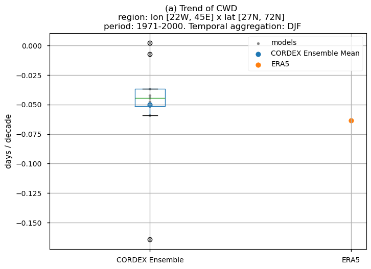
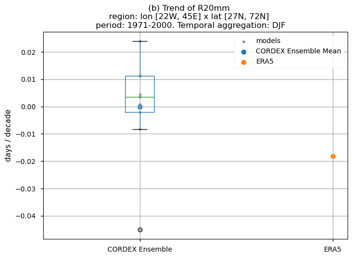
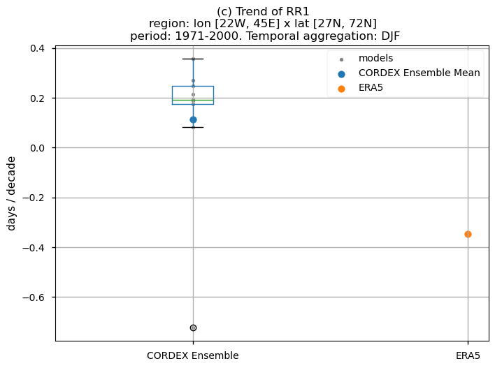
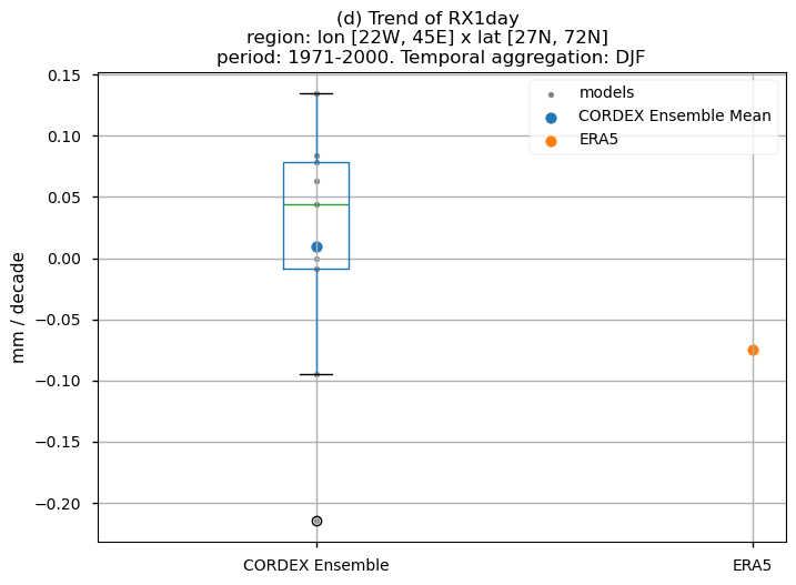
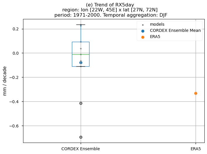
Fig 31. Boxplots illustrating the historical trends of the ensemble distribution and ERA5 for the precipitation-based indices: (a)'CWD', (b)'R20mm', (c)'RR1', (d)'RX1day' and (e)'RX5day'. The distribution is created by considering spatially averaged trends across Europe. The ensemble mean and the ensemble median trends are both included. Outliers in the distribution are denoted by a grey circle with a black contour.
3.6. Results summary and discussion#
The bias behaviour varies depending on the index and whether we are dealing with trends or climatologies. Generally speaking, the subset of models selected overestimates the magnitudes of climatologies for DJF, except in the northwest of Great Britain, the west coast of the Scandinavian Peninsula, parts of the Mediterranean Basin, and the east of Europe for the CWD index, where there is underestimation. For the RR1 index, the models also underestimate the magnitudes for the west coast of the Scandinavian Peninsula and parts of the Mediterranean Basin.
For the historical period and the seasonal aggregation of DJF, ERA5 exhibits trends that are highly dependent on the region and index. Indices like CWD, R20mm, and RX1day show scattered spatial patterns that are generally not well-reproduced by the considered models, except in some specific areas. The spatial patterns for the trends of RR1 and RX5day are less scattered and are slightly better captured than those of the other indices.
The boxplots displaying spatially-averaged values reveal diverse outcomes depending on the index under consideration. Notably, significant inter-model variability is evident for certain indices, whose interquantile range encompasses trends of varying directions, and in some cases, even exhibits a trend opposite to that shown by the ERA5 data. This discrepancy is particularly noticeable for the R20mm, RR1, and RX1day indices, where the interquantile range showcases a trend contrary to that portrayed by ERA5. Meanwhile, the RX5day index displays an interquantile range centered around zero, with the trend sign dependent on the model. In contrast, the CWD index demonstrates a trend direction consistent with ERA5.
It is crucial to emphasise that the boxplots present spatially-averaged values, and their interpretation should be approached with caution, as the outcomes can vary significantly when considering different regions across Europe. For regional analyses, it is essential to focus solely on the region of interest, as the influence of other European regions may distort the results, leading to conclusions that do not accurately reflect the specific area under study.
Although ERA5 is used as our reference dataset, it is important to be aware of its inherent uncertainties. While uncertainties affect all variables, biases are particularly pronounced for variables such as surface wind and precipitation, as demonstrated in [4] and [5]. This underscores the importance of careful interpretation, especially regarding precipitation extremes.
A larger GCM-RCM matrix should be considered when addressing specific cases to enhance the robustness of the analysis and account for uncertainties [6][7].
What do the results mean for users? Are the biases relevant?
The subset of Regional Climate Models (RCMs) considered for this notebook and for this seasonal aggregation struggle to replicate both the observed climatology and the trends during the historical period, with particular difficulty in capturing the trends.
However, for specific regions and indices, the models successfully capture the climatology and even the direction of the trend. Examples include the increasing trend for the CWD index in the western part of the Iberian Peninsula and the positive trend for RR1 in central Europe. Users should consider these regional variations, the indices they aim to use, the differences in bias behavior between climatology and trends, and the necessity of bias-correcting data before using it for hydrological applications [3].
Precipitation trends in observational and reanalysis datasets are generally less robust and more challenging to detect compared to temperature trends. This limitation is also evident in model simulations.
It is important to note that the results presented are specific to the 9 models chosen, and users should aim to assess as wide a range of models as possible before making a sub-selection.
If you want to know more#
Key resources#
Some key resources and further reading were linked throughout this assessment.
The CDS catalogue entries for the data used were:
CORDEX regional climate model data on single levels (Daily mean - Mean precipitation flux): https://cds.climate.copernicus.eu/cdsapp#!/dataset/projections-cordex-domains-single-levels?tab=overview
ERA5 hourly data on single levels from 1940 to present (Total precipitation): https://cds.climate.copernicus.eu/cdsapp#!/dataset/reanalysis-era5-single-levels?tab=overview
Code libraries used:
C3S EQC custom functions,
c3s_eqc_automatic_quality_control, prepared by BOpenicclim Python package
References#
[1] Panagos, P., Borrelli, P., Poesen, J., Ballabio, C., Lugato, E., Meusburger, K., Montanarella, L., Alewell, C. (2015). The new assessment of soil loss by water erosion in Europe. Environ. Sci. Policy, 54, pp. 438-447. https://doi.org/10.1016/j.envsci.2015.08.012
[2] Salvati, L., Carlucci, M. (2013). The impact of mediterranean land degradation on agricultural income: a short-term scenario. Land Use Policy, 32, pp. 302-308. https://doi.org/10.1016/j.landusepol.2012.11.007
[3] Teutschbein, C., Seibert, J. (2012). Bias correction of regional climate model simulations for hydrological climate-change impact studies: Review and evaluation of different methods. Journal of Hydrology, Volumes 456–457, pp. 12-29. https://doi.org/10.1016/j.jhydrol.2012.05.052
[4] Ramon, J., Lledó L., Torralba, V., Soret, A., Doblas-Reyes, F.J. (2019). What global reanalysis best represents near-surface winds?. Q J R Meteorol Soc. 2019; 145: 3236–3251. https://doi.org/10.1002/qj.3616
[5] Hassler, B. and Lauer, A. (2021). Comparison of Reanalysis and Observational Precipitation Datasets Including ERA5 and WFDE5. Atmosphere, 12, 1462. https://doi.org/10.3390/atmos12111462
[6] Rummukainen, M. (2010). State-of-the-art with regional climate models. WIREs Clim Change, 1: 82-96. https://doi.org/10.1002/wcc.8
[7] Silje Lund Sørland et al. (2018). Bias patterns and climate change signals in GCM-RCM model chains. Environ. Res. Lett. 13 074017. https://doi.org/10.1088/1748-9326/aacc77