Please note that this repository is used for development and review, so quality assessments should be considered work in progress until they are merged into the main branch

1.1.1. Satellite Earth’s outgoing longwave and shortwave radiation budget intercomparison for climate monitoring

Production date: 11-06-2025

Last Review: 20-02-2026

Produced by: CNR-ISMAR, Andrea Storto, Vincenzo de Toma, Claudia Allegrini and Gian Luigi Liberti

🌍 Use case: Consistency assessment of Earth Radiation Budget products

❓ Quality assessment question(s)

• How consistent are the Earth Radiation Budget products provided by C3S?

The Earth Radiation Budget (ERB) Outgoing Longwave Radiation (OLR) and Outgoing Shortwave Radiation (OSR) products provide estimates of the radiative flux components leaving the Earth system at the top of the atmosphere (TOA), and are fundamental for climate monitoring and model evaluation. These quantities are also central for estimating the Earth’s Energy Imbalance (EEI), evaluating climate feedbacks, and attributing climate variability and change. Despite their common physical target, ERB products differ substantially in terms of satellite sensors, spectral coverage, angular-distribution models, calibration strategies, spatial resolution, temporal coverage, swath width, and gap-filling approaches. These differences directly affect data quality, particularly in regions characterised by strong angular anisotropy, complex cloud regimes, or persistent data gaps, such as the polar regions and areas with frequent deep convection. Consequently, inter-comparison of ERB products requires careful consideration of their respective retrieval methodologies and sampling characteristics, as well as explicit attention to data quality aspects such as spatial completeness, temporal homogeneity, and sensitivity to surface and cloud conditions ([1], [2], [3], [4]).

📢 Quality assessment statement

These are the key outcomes of this assessment

• Important differences among products arise from well-documented characteristics of the underlying instruments and retrieval algorithms, including spectral sampling, angular-distribution models, cloud detection, calibration stability, and, more generally, steps of the processing chain. These differences are most pronounced at high latitudes, over bright surfaces, and in persistently cloudy regions, where uncertainties in anisotropy corrections and cloud properties are largest ([2], [3], [5]).

• Products with limited temporal coverage or without gap-filling (e.g.ERS-2, ENVISAT, Sentinel) exhibit reduced suitability for applications requiring closed global energy budgets, such as direct estimation of Earth’s Energy Imbalance, unless additional assumptions or data fusion approaches are applied ([4], [6]).

• The combined use of multiple ERB products is therefore recommended only for advanced users and for carefully selected periods and applications, with explicit consideration of data quality limitations documented in the respective product validation reports.

• Spatial patterns in some products, particularly those derived from narrow‐swath instruments (e.g. ERS‐2 ATSR‐2/AATSR), exhibit sampling‐related artefacts such as track‐like features in time‐mean and bias maps. These features are the footprint of representativeness limitations associated with the swath width and the orbital sampling rather than systematic retrieval biases, and are reduced in wide‐swath products such as AVHRR‐based CLARA‐A3, CERES, HIRS, or Sentinel ([2], [3]).

As one of the main outcomes of this assessment, we provide the synthesis given by the construction of the globally averaged time series of monthly mean Net Top of the Atmosphere Radiation (see description in the Methodology section for its calculation). There are two main features: the sharp peak in ERS-2 data at the beginning of the time series, and another peak in 2020. The first one can be explained by the switch of the Near Infra Red channel onboard of NOAA satellites (from 3.7 to 1.6 micrometres), while the second feature is due to a known bias of Sentinel products in both components (about 6 W m^-2 for the OLR, and about 4 W m^-2 for the OSR).

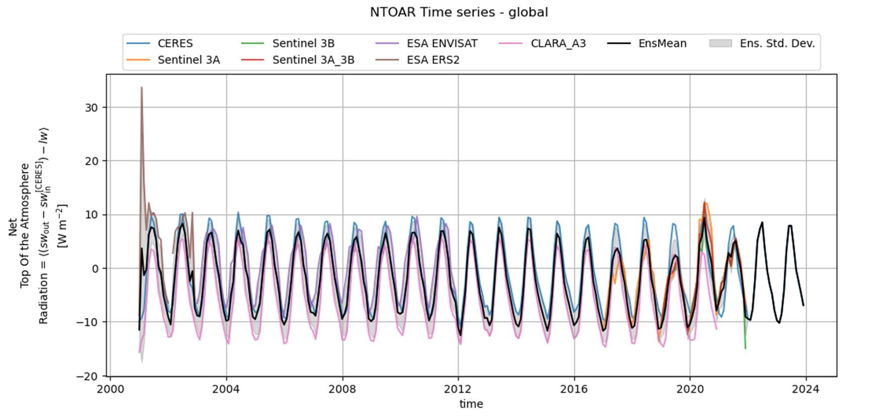
Fig. 1.1.1.1 Monthly mean time series Net Top Of the Atmosphere Radiation (NTOAR) globally averaged. The ensemble mean is reported in black, with grey shading indicating the ensemble standard deviation, and a different colour represents each product (see methodology below).

📋 Methodology

In this notebook, we inter-compare the following Earth Radiation Budget Products, available through the Climate Data Store (CDS) by C3S:

1. NASA CERES EBAF (CERES): The Cloud and Earth’s Radiant Energy System (CERES) Energy Balanced And Filled (EBAF) provides a state-of-the-art Climate Data Record (CDR) of monthly mean top-of-atmosphere radiative fluxes, with global (1 degree spatial resolution) coverage. Here we consider only complete years, so the time coverage spans from January 2001 to December 2023.

2. NOAA/NCEI HIRS OLR (HIRS): produced by the NOAA/NCEI from the High Resolution Infrared Radiation Sounder instruments on board the NOAA and MetOp satellites, and new generation infrared hyperspectral sounder radiance data, including from the Infrared Atmospheric Sounding Interferometer (IASI) since 2007 and the Cross-track Infrared Sounder (CrIS) since 2012. Here, we assess monthly means of the Outgoing Longwave Radiation (OLR) with global (2.5 degrees spatial resolution) coverage, spanning from January 1979 to December 2023.

3. EUMETSAT CLARA-A3 (CLARA-A3): The “CLARA product family” refers to European Organisation for the Exploitation of Meteorological Satellites CM SAF CLARA-A3 data record (CM SAF cLoud, Albedo and surface RAdiation dataset from AVHRR data - Edition 3). It merges the AVHRR-sensor data from a variety of satellites into a combined TCDR. Here, we assess the monthly means of TOA Reflected Solar Flux and TOA Outgoing Longwave Radiation, with global (0.25 degree spatial resolution) coverage, spanning from January 1979 to December 2020.

4. ESA/C3S CCI (ESA ERS2, ESA ENVISAT, SENTINEL 3A, SENTINEL 3B, SENTINEL 3A_3B): The CCI product family refers to the European Space Agency Cloud_cci Earth radiation data record, with global (0.5 degree spatial resolution) coverage. This record comprises observations from the Along Track Scanning Radiometer (ATSR) series of instruments, flown onboard ESA Earth Observation satellites, ERS-2 (spanning complete years from January 1997 to December 2002), and Envisat (spanning from January 2003 to December 2011). The Copernicus Climate Change Service (C3S) part covers the Interim Climate Data Record (ICDR) extension of the ESA Cloud_cci dataset. It is based on observations from the Sea and Land Surface Temperature Radiometer (SLSTR), flown on board the ESA Sentinel 3A (spanning from January 2017 to December 2021) and 3B satellites (spanning from January 2019 to December 2012). In addition to data from each individual satellite, a merged product from both satellites is also provided from the launch of Sentinel-3B (a complete-year period spanning from January 2019 to December 2021).

CERES is the only product which gives also the incoming shortwave radiation: thus, to evaluate the Net Top Of the Atmosphere Radiation (which we consider here to be close to the Earth’s Energy Imbalance due to missing data), the ensemble mean budget was built using outgoing longwave and outgoing shortwave from each product, and the incoming shortwave from CERES, and then averaging across the product dimension.

The analysis and results are organised in the following steps, which are detailed in the sections below:

1. Choose the data to use and setup code

2. Download and transform

3. Spatial weighted means and anomaly scatter plots

4. Plot time weighted means

5. Plot spatial weighted zonal means

📈 Analysis and results

1. Choose the data to use and setup code

In this section, we import the required packages and define the dataset names for use in the following sections. Processing functions are also defined. We select only complete years for each dataset to ensure a fair comparison across products. Ancillary functions and corresponding keyword arguments to preprocess inhomogeneities along the time dimension are also defined here. We also define a set of regions to investigate time-series of spatially averaged anomalies and climatologies: the global domain (0,360 for longitude, -90,90 for latitude), the northern high-latitudes (60,90 for latitude, 0,360 for longitude), the northern mid-latitudes (30,60 for latitude, 0,360 for longitude), the tropics (-30,30 for latitude, 0,360 for longitude) and southern analogues.

Show code cell source

Hide code cell source

import os
os.environ["CDSAPI_RC"] = os.path.expanduser("~/detoma_vincenzo/.cdsapirc")
import xarray as xr
import pandas as pd
import matplotlib.pyplot as plt
import numpy as np
import datetime
from cartopy import crs as ccrs, feature as cfeature
import cartopy.mpl.ticker as cticker
from c3s_eqc_automatic_quality_control import download, plot, utils, diagnostics
import warnings
warnings.filterwarnings("ignore")

# Variable to analyse
variables = ["outgoing_longwave", "outgoing_shortwave", "incoming_shortwave"]
request_dicts = []

for variable in variables:

    # Region for timeseries
    region_slices = {
        "global": {"lat_slice": slice(-90, 90), "lon_slice": slice(0, 360)},
        "northern high-latitudes": {"lat_slice": slice(60, 90), "lon_slice": slice(0, 360)},
        "northern mid-latitudes": {"lat_slice": slice(30, 60), "lon_slice": slice(0, 360)},
        "tropics" : {"lat_slice": slice(-30, 30), "lon_slice": slice(0, 360)},
        "southern mid-latitudes": {"lat_slice": slice(-60, -30), "lon_slice": slice(0, 360)},
        "southern high-latitudes": {"lat_slice": slice(-90, -60), "lon_slice": slice(0,360)},
    }

    collection_id = "satellite-earth-radiation-budget"
    chunks = {"year": 1}
    varnames = (
        {"olr", "toa_lw_all_mon"} if variable == "outgoing_longwave" else {"rsf", "toa_sw_all_mon"}
    )

    collection_id = "satellite-earth-radiation-budget"
    chunks = {"year": 1}
    varnames = (
        {"olr", "toa_lw_all_mon", "LW_flux"}
        if variable == "outgoing_longwave"
        else {"rsf", "toa_sw_all_mon", "SW_flux"}
    )

    request_dict = {
        "CERES": {
            "start": "2001-01",
            "stop": "2023-12",
            "product_family": "ceres_ebaf",
            "climate_data_record_type": "thematic_climate_data_record",
            "time_aggregation": "monthly_mean",
            "format": "zip",
            "origin": "nasa",
            "variable": f"{variable}_radiation",
        },
        "Sentinel 3A": {
            "start": "2017-01",
            "stop": "2021-12",
            "format": "zip",
            "origin": "c3s",
            "sensor_on_satellite": "slstr_on_sentinel_3a",
            "variable": "all_variables",
            "product_family": "cci",
            "time_aggregation": "monthly_mean",
            "climate_data_record_type": "interim_climate_data_record",
        },
        "Sentinel 3B": {
            "start": "2019-01",
            "stop": "2021-12",
            "format": "zip",
            "origin": "c3s",
            "sensor_on_satellite": "slstr_on_sentinel_3b",
            "variable": "all_variables",
            "product_family": "cci",
            "time_aggregation": "monthly_mean",
            "climate_data_record_type": "interim_climate_data_record",
        },
        "Sentinel 3A_3B": {
            "start": "2019-01",
            "stop": "2021-12",
            "format": "zip",
            "origin": "c3s",
            "sensor_on_satellite": "slstr_on_sentinel_3a_3b",
            "variable": "all_variables",
            "product_family": "cci",
            "time_aggregation": "monthly_mean",
            "climate_data_record_type": "interim_climate_data_record",
        },
        "ESA ENVISAT": {
            "start": "2003-01",
            "stop": "2011-12",
            "format": "zip",
            "origin": "esa",
            "product_family": "cci",
            "climate_data_record_type": "thematic_climate_data_record",
            "time_aggregation": "monthly_mean",
            "sensor_on_satellite": "aatsr",
            "variable": "all_variables",
        },
        "ESA ERS2": {
            "start": "1997-01",
            "stop": "2002-12",
            "format": "zip",
            "origin": "esa",
            "sensor_on_satellite": "atsr2",
            "time_aggregation": "monthly_mean",
            "product_family": "cci",
            "climate_data_record_type": "thematic_climate_data_record",
            "variable": "all_variables",
        },
        "CLARA_A3": {
            "start": "1979-01",
            "stop": "2020-12",
            "product_family": "clara_a3",
            "origin": "eumetsat",
            "variable": f"{variable}_radiation",
            "climate_data_record_type": "thematic_climate_data_record",
            "time_aggregation": "monthly_mean",
        },
        "HIRS": {
            "start": "1979-01",
            "stop": "2023-12",
            "format": "zip",
            "origin": "noaa_ncei",
            "product_family": "hirs",
            "climate_data_record_type": "thematic_climate_data_record",
            "time_aggregation": "monthly_mean",
            "version": "2_7_reprocessed",
            "variable": f"{variable}_radiation",
        },
    }
    request_dicts.append(request_dict)

def preprocess_time(ds):
    if "time" in ds and "units" in ds["time"].attrs:
        # Could not decode
        ds = ds.squeeze("time", drop=True)
    if "time" not in ds:
        time = pd.to_datetime(ds.attrs["time_coverage_start"].replace("Z", ""))
        ds = ds.expand_dims(time=[time])
    return ds


xarray_kwargs = {
    "drop_variables": ["time_bounds", "record_status"],
    "preprocess": preprocess_time,
}

In the following cell, we redefine the spatial weighted mean to account for the possibility of masking data and allow changing the default behaviour for treating NaNs.

Show code cell source

Hide code cell source

# Re-define spatial_weighted_mean to apply common masks on the target grid
def spatial_weighted_mean(ds, lon_slice, lat_slice, regrid, ds_obj, SKIP, mask=None):
    if mask is None:
        if regrid==True:
            ds = diagnostics.regrid(ds, ds_obj, method='bilinear', skipna=SKIP)
        ds = utils.regionalise(ds, lon_slice=lon_slice, lat_slice=lat_slice)
        return diagnostics.spatial_weighted_mean(ds, weights=True, skipna=SKIP)
    else:
        if regrid==True:
            ds = diagnostics.regrid(ds, ds_obj, method='bilinear', skipna=SKIP)
            mask = diagnostics.regrid(mask, ds_obj, method='bilinear', skipna=SKIP)
        ds = utils.regionalise(ds, lon_slice=lon_slice, lat_slice=lat_slice)
        mask = utils.regionalise(mask, lon_slice=lon_slice, lat_slice=lat_slice)
        return diagnostics.spatial_weighted_mean(ds.where(~np.isnan(mask)), weights=True, skipna=SKIP)

2. Download and transform

The code below will download the products. Notice the definition of common periods for the different products, and their inclusion in the mean map dictionary. A custom function to build the mean map over a specified period is also defined here. When the variable to download is the shortwave component, we skip the HIRS dataset because only the longwave is available in it. Moreover, incoming shortwave radiation is only available for CERES data.

Show code cell source

Hide code cell source

weights=True
skipna=True
p = []
start_var = {}
stop_var = {}
DS = {}
for variable, request_dict in zip(variables, request_dicts):
    Ds = {}
    start_prod = {}
    stop_prod = {}
    for product, request in request_dict.items():
        if product == "HIRS" and variable != "outgoing_longwave":
            continue
        if "CERES" not in product and variable=="incoming_shortwave":
            continue
        p.append(product)
    
        start = request.pop("start")
        stop = request.pop("stop")
        start_prod[product] = start
        stop_prod[product] = stop
        
        requests = download.update_request_date(
            request, start=start, stop=stop, stringify_dates=True
        )
    
        ds = download.download_and_transform(
            collection_id,
            requests,
            chunks=chunks,
            transform_chunks=False,
            **xarray_kwargs,
            quiet=True,
        )
        Ds[product] = ds
    start_var[variable] = start_prod
    stop_var[variable] = stop_prod
    DS[variable] = Ds

clara_a3_start, clara_a3_end ="1980-01", "2020-12"
ceres_start, ceres_end = "2001-01", "2023-12"
esa_envisat_start, esa_envisat_end = "2003-01", "2011-12" 
sentinel_start, sentinel_end = "2019-01", "2021-12"
esa_ers2_start, esa_ers2_end = "1997-01", "2002-12"

def mean_map_period(ds, start, stop, W, S):
    selection = ds.sel(time=slice(start, stop))
    time_coord =  np.array(pd.date_range(start, stop, freq='MS'), dtype=np.datetime64)
    ds = selection.assign_coords({'time':('time', time_coord, selection.time.attrs)})
    ds_map = diagnostics.time_weighted_mean(ds, weights=W, skipna=S)
    return ds_map

In the following cell, we define functions to ease the handling of different variable names and to homogenise the longitude dimension. Then, we build mean maps across overlapping periods, without masking them for now, since we’ll use them to create common masks for each period.

Show code cell source

Hide code cell source

def get_varname(ds, variable):
    if variable=="outgoing_longwave":
        varnames = (
            {"olr", "toa_lw_all_mon", "LW_flux"}
        )
    elif variable=="outgoing_shortwave":
        varnames = (
            {"rsf", "toa_sw_all_mon", "SW_flux"}
        )
    else:
        varnames = (
            {"solar_mon"}
        )
        
    (varname,) = set(ds.data_vars) & varnames
    return varname

def fix_lon_0_360(da, lon_name="longitude"):
    """
    Convert longitude coordinates from [-180, 180] to [0, 360).

    Parameters
    ----------
    da : xr.DataArray or xr.Dataset
        Input object with a longitude coordinate.
    lon_name : str
        Name of the longitude coordinate.

    Returns
    -------
    xr.DataArray or xr.Dataset
        Object with longitudes in [0, 360).
    """
    lon = da[lon_name]

    # Check if longitudes look like [-180, 180]
    if lon.min() < 0:
        da = da.assign_coords(
            {lon_name: (lon % 360)}
        ).sortby(lon_name)

    return da

ds_maps = {}
ds_maps_p1 = {}
ds_maps_p2 = {}
ds_maps_p3 = {}
ds_maps_p4 = {}
ds_maps_p5 = {}
p = []
for variable, request_dict in zip(variables, request_dicts):
    da_maps = {}
    da_maps_p1 = {}
    da_maps_p2 = {}
    da_maps_p3 = {}
    da_maps_p4 = {}
    da_maps_p5 = {}
    for product, request in request_dict.items():
        if product == "HIRS" and variable != "outgoing_longwave":
            continue
        if "CERES" not in product and variable=="incoming_shortwave":
            continue
        p.append(product)
    
        start = start_var[variable][product]
        stop = stop_var[variable][product]

        ds = DS[variable][product]
        
        varname=get_varname(ds, variable)
        
        da = ds[varname]
        if product=="CERES":
            regrid=False
            da_obj = ds[varname]
        else:
            regrid=True
            da = diagnostics.regrid(da, da_obj, method='bilinear')
        da.attrs.update({"start": start, "stop": stop})
        da = fix_lon_0_360(da)
        da_maps[product] = diagnostics.time_weighted_mean(da, weights=True, skipna=True)

        curr_time = pd.date_range(start, stop)
        ceres_time = pd.date_range(ceres_start, ceres_end)
        clara_a3_time = pd.date_range(clara_a3_start, clara_a3_end)
        esa_envisat_time = pd.date_range(esa_envisat_start, esa_envisat_end)
        sentinel_time = pd.date_range(sentinel_start, sentinel_end)
        esa_ers2_time = pd.date_range(esa_ers2_start, esa_ers2_end)
        if clara_a3_time[0] in curr_time and clara_a3_time[-1] in curr_time:
            da_maps_p1[product] = mean_map_period(da, clara_a3_start, clara_a3_end, W=weights, S=skipna)
            da_maps_p1[product] = diagnostics.regrid(da_maps_p1[product].rename(variable), da_obj, method='bilinear')
        if ceres_time[0] in curr_time and ceres_time[-1] in curr_time:
            da_maps_p2[product] = mean_map_period(da, ceres_start, ceres_end, W=weights, S=skipna)
            da_maps_p2[product] = diagnostics.regrid(da_maps_p2[product].rename(variable), da_obj, method='bilinear')
        if esa_envisat_time[0] in curr_time and esa_envisat_time[-1] in curr_time:
            da_maps_p3[product] = mean_map_period(da, esa_envisat_start, esa_envisat_end, W=weights, S=skipna) 
            da_maps_p3[product] = diagnostics.regrid(da_maps_p3[product].rename(variable), da_obj, method='bilinear')
        if sentinel_time[0] in curr_time and sentinel_time[-1] in curr_time:
            da_maps_p4[product] = mean_map_period(da, sentinel_start, sentinel_end, W=weights, S=skipna) 
            da_maps_p4[product] = diagnostics.regrid(da_maps_p4[product].rename(variable), da_obj, method='bilinear')
        if esa_ers2_time[0] in curr_time and esa_ers2_time[-1] in curr_time:
            da_maps_p5[product] = mean_map_period(da, esa_ers2_start, esa_ers2_end, W=weights, S=skipna) 
            da_maps_p5[product] = diagnostics.regrid(da_maps_p5[product].rename(variable), da_obj, method='bilinear')

    ds_maps_p1[variable] = da_maps_p1
    ds_maps_p2[variable] = da_maps_p2
    ds_maps_p3[variable] = da_maps_p3
    ds_maps_p4[variable] = da_maps_p4
    ds_maps_p5[variable] = da_maps_p5
    ds_maps[variable] = da_maps

Here, we gather periods together and define functions to build a common mask for each period, then put them together.

Show code cell source

Hide code cell source

# Build common masks for each overlapping period before further calculations
ds_periods_list = [ds_maps_p1, ds_maps_p2, ds_maps_p3, ds_maps_p4, ds_maps_p5]
periods = [clara_a3_time, ceres_time, esa_envisat_time, sentinel_time, esa_ers2_time]

def build_common_mask(ds_maps_var):
    products = list(ds_maps_var.keys())
    if len(products) == 0:
        return None
    mask = xr.concat(
        [xr.where(~np.isnan(ds_maps_var[p]), 1, np.nan) for p in products],
        dim="product",
    )
    return mask.min("product", skipna=False)

masks_periods = []
for ds_maps in ds_periods_list:
    mask_dict = {}
    for variable in ["outgoing_longwave", "outgoing_shortwave"]:
        if variable not in ds_maps:
            continue
        mask_var = build_common_mask(ds_maps[variable])
        if mask_var is not None:
            mask_dict[variable] = mask_var
    if len(mask_dict) == 0:
        masks_periods.append(None)
        continue
    mask_period = xr.concat(
        [mask_dict[v] for v in mask_dict.keys()],
        dim="variable",
    ).assign_coords({"variable": list(mask_dict.keys())})
    masks_periods.append(mask_period)

period_masks = {
    "CLARA-A3": masks_periods[0],
    "CERES": masks_periods[1],
    "ESA-ENVISAT": masks_periods[2],
    "Sentinel-3": masks_periods[3],
    "ESA-ERS2": masks_periods[4],
}
listmasks = [ds_maps[k] for k in ds_maps.keys()]

Here, we build the time series over specified common periods, with appropriate masking.

Show code cell source

Hide code cell source

ds_timeseries = {}
ds_timeseries_p1 = {}
ds_timeseries_p2 = {}
ds_timeseries_p3 = {}
ds_timeseries_p4 = {}
ds_timeseries_p5 = {}
p = []

def get_period_mask(label, variable):
    mask_period = period_masks.get(label)
    if mask_period is None:
        return None
    if "variable" in mask_period.dims and variable in mask_period.variable.values:
        return mask_period.sel(variable=variable)
    return None

def build_regional_timeseries(da, mask_common, regrid, ds_obj, SKIP):
    dataarrays = []
    for region, slices in region_slices.items():
        dall = {}
        dall.update(slices)
        dall.update({'regrid': regrid, 'ds_obj': ds_obj, 'SKIP': SKIP})
        da_ts = spatial_weighted_mean(
            da,
            lon_slice=dall['lon_slice'],
            lat_slice=dall['lat_slice'],
            regrid=dall['regrid'],
            ds_obj=dall['ds_obj'],
            SKIP=dall['SKIP'],
            mask=mask_common,
        )
        dataarrays.append(da_ts.expand_dims(region=[region]))
    return xr.concat(dataarrays, "region")

def build_period_timeseries(da, start, end, mask_common, regrid, ds_obj, SKIP):
    da_sel = da.sel(time=slice(start, end))
    da_ts = build_regional_timeseries(da_sel, mask_common, regrid, ds_obj, SKIP)
    da_ts = da_ts.assign_coords({'time': np.array(pd.date_range(start, end, freq='MS'), dtype=np.datetime64)})
    return da_ts

def get_overlap_range(da, start, end):
    if "time" not in da.dims or da.time.size == 0:
        return None
    tmin = pd.to_datetime(da.time.min().values)
    tmax = pd.to_datetime(da.time.max().values)
    start_ts = pd.to_datetime(start)
    end_ts = pd.to_datetime(end)
    if tmax < start_ts or tmin > end_ts:
        return None
    overlap_start = max(tmin, start_ts).strftime("%Y-%m")
    overlap_end = min(tmax, end_ts).strftime("%Y-%m")
    return overlap_start, overlap_end

# Period-specific inclusion lists for annual-cycle plots
period_products = {
    "CLARA-A3": {"CLARA_A3", "HIRS"},
    "CERES": {"CERES", "HIRS"},
    "ESA-ENVISAT": {"ESA ENVISAT", "CERES", "HIRS", "CLARA_A3"},
    "Sentinel-3": {"CERES", "Sentinel 3A", "Sentinel 3B", "Sentinel 3A_3B", "HIRS"},
    "ESA-ERS2": {"ESA ERS2", "HIRS", "CLARA_A3"},
}

for variable, request_dict in zip(variables, request_dicts):
    da_timeseries = {}
    da_timeseries_p1 = {}
    da_timeseries_p2 = {}
    da_timeseries_p3 = {}
    da_timeseries_p4 = {}
    da_timeseries_p5 = {}
    for product, request in request_dict.items():
        if product == "HIRS" and variable != "outgoing_longwave":
            continue
        if "CERES" not in product and variable == "incoming_shortwave":
            continue
        p.append(product)

        start = start_var[variable][product]
        stop = stop_var[variable][product]

        ds = DS[variable][product]

        varname = get_varname(ds, variable)

        da = ds[varname]
        if product == "CERES":
            regrid = False
            da_obj = ds[varname]
        else:
            regrid = True
            da = diagnostics.regrid(da, da_obj, method='bilinear')
        da.attrs.update({"start": start, "stop": stop})

        mask_da = da.mean("time", skipna=True)
        da_full = build_regional_timeseries(da, mask_da, regrid, da_obj, SKIP=True)
        da_full.attrs.update({"start": start, "stop": stop})
        da_timeseries[product] = da_full.rename(variable)

        overlap = get_overlap_range(da, clara_a3_start, clara_a3_end)
        if overlap is not None and product in period_products["CLARA-A3"]:
            mask_common = get_period_mask("CLARA-A3", variable)
            da_timeseries_p1[product] = build_period_timeseries(
                da, overlap[0], overlap[1], mask_common, regrid, da_obj, SKIP=True
            ).rename(variable)
        overlap = get_overlap_range(da, ceres_start, ceres_end)
        if overlap is not None and product in period_products["CERES"]:
            mask_common = get_period_mask("CERES", variable)
            da_timeseries_p2[product] = build_period_timeseries(
                da, overlap[0], overlap[1], mask_common, regrid, da_obj, SKIP=True
            ).rename(variable)
        overlap = get_overlap_range(da, esa_envisat_start, esa_envisat_end)
        if overlap is not None and product in period_products["ESA-ENVISAT"]:
            mask_common = get_period_mask("ESA-ENVISAT", variable)
            da_timeseries_p3[product] = build_period_timeseries(
                da, overlap[0], overlap[1], mask_common, regrid, da_obj, SKIP=True
            ).rename(variable)
        overlap = get_overlap_range(da, sentinel_start, sentinel_end)
        if overlap is not None and product in period_products["Sentinel-3"]:
            mask_common = get_period_mask("Sentinel-3", variable)
            da_timeseries_p4[product] = build_period_timeseries(
                da, overlap[0], overlap[1], mask_common, regrid, da_obj, SKIP=True
            ).rename(variable)
        overlap = get_overlap_range(da, esa_ers2_start, esa_ers2_end)
        if overlap is not None and product in period_products["ESA-ERS2"]:
            mask_common = get_period_mask("ESA-ERS2", variable)
            da_timeseries_p5[product] = build_period_timeseries(
                da, overlap[0], overlap[1], mask_common, regrid, da_obj, SKIP=True
            ).rename(variable)
    ds_timeseries_p1[variable] = da_timeseries_p1
    ds_timeseries_p2[variable] = da_timeseries_p2
    ds_timeseries_p3[variable] = da_timeseries_p3
    ds_timeseries_p4[variable] = da_timeseries_p4
    ds_timeseries_p5[variable] = da_timeseries_p5
    ds_timeseries[variable] = da_timeseries

Here, we define a function to ensure all datasets share the same time convention.

Show code cell source

Hide code cell source

def fix_time(ds):
    t = ds.time.to_index().to_period("M").to_timestamp()
    ds = ds.assign_coords(time=t)
    return ds

for v in variables:
    for ds in [ds_timeseries, ds_timeseries_p1, ds_timeseries_p2, ds_timeseries_p3, ds_timeseries_p4, ds_timeseries_p5]:
        for k in ds[v].keys():
            ds[v][k] = fix_time(ds[v][k])

3. Spatial weighted means and anomaly scatter plots

Below, we calculate and plot spatially weighted means for the different earth radiation budget products, in terms of monthly climatologies, although the sampling period of each dataset is, in general, different from the others (i.e. CERES: 2001-2023, Sentinel 3A: 2017-2021, Sentinel 3B: 2019-2021, Sentinel 3A_3B: 2019-2021, ESA_Envisat: 2003-2011, CLARA_A3: 1979-2020, HIRS: 1979-2023). We therefore selected a set of periods of common overlaps in which to carry out this comparison. The same periods will be used for other diagnostics, such as the mean maps and the zonal mean monthly-climatological profiles.

The pronounced seasonality in OLR is mostly linked to the larger land area in the Northern Hemisphere, whereas that in OSR is mainly linked to the solar cycle.

Show code cell source

Hide code cell source

def concat_ts(ts_dict, allowed_products=None):
    if ts_dict is None or len(ts_dict) == 0:
        return None
    products = list(ts_dict.keys()) if allowed_products is None else [p for p in allowed_products if p in ts_dict]
    if len(products) == 0:
        return None
    ts = xr.concat(
        [ts_dict[k] for k in products],
        dim='product',
    ).assign_coords({'product': products})
    return ts

lw_products = list(ds_timeseries['outgoing_longwave'].keys())
sw_products = list(ds_timeseries['outgoing_shortwave'].keys())

lw_ts = concat_ts(ds_timeseries['outgoing_longwave'], lw_products)
sw_ts = concat_ts(ds_timeseries['outgoing_shortwave'], sw_products)

lw_ts_p1 = concat_ts(ds_timeseries_p1['outgoing_longwave'])
lw_ts_p2 = concat_ts(ds_timeseries_p2['outgoing_longwave'])
lw_ts_p3 = concat_ts(ds_timeseries_p3['outgoing_longwave'])
lw_ts_p4 = concat_ts(ds_timeseries_p4['outgoing_longwave'])
lw_ts_p5 = concat_ts(ds_timeseries_p5['outgoing_longwave'])

sw_ts_p1 = concat_ts(ds_timeseries_p1['outgoing_shortwave'])
sw_ts_p2 = concat_ts(ds_timeseries_p2['outgoing_shortwave'])
sw_ts_p3 = concat_ts(ds_timeseries_p3['outgoing_shortwave'])
sw_ts_p4 = concat_ts(ds_timeseries_p4['outgoing_shortwave'])
sw_ts_p5 = concat_ts(ds_timeseries_p5['outgoing_shortwave'])

periods_info = [
    ("CLARA-A3", clara_a3_start, clara_a3_end),
    ("CERES", ceres_start, ceres_end),
    ("ESA-ENVISAT", esa_envisat_start, esa_envisat_end),
    ("Sentinel-3", sentinel_start, sentinel_end),
    ("ESA-ERS2", esa_ers2_start, esa_ers2_end),
 ]

lw_ts_periods = {
    "CLARA-A3": lw_ts_p1,
    "CERES": lw_ts_p2,
    "ESA-ENVISAT": lw_ts_p3,
    "Sentinel-3": lw_ts_p4,
    "ESA-ERS2": lw_ts_p5,
}
sw_ts_periods = {
    "CLARA-A3": sw_ts_p1,
    "CERES": sw_ts_p2,
    "ESA-ENVISAT": sw_ts_p3,
    "Sentinel-3": sw_ts_p4,
    "ESA-ERS2": sw_ts_p5,
}

Here, we define the function to plot the monthly climatology over the specified period.

Show code cell source

Hide code cell source

def plot_period_climatology(ts, period_label, start, stop, title_prefix):
    if ts is None or ts.sizes.get('product', 0) <= 1:
        return
    climatology = ts.groupby('time.month').mean('time')
    t = climatology.plot(col='region', col_wrap=3, hue='product', figsize=(10, 6), marker='o', markeredgecolor='k')
    for ax in t.axs.flatten():
        ax.set_xticks([1, 2, 3, 4, 5, 6, 7, 8, 9, 10, 11, 12])
        ax.set_xticklabels(['Jan', 'Feb', 'Mar', 'Apr', 'May', 'Jun', 'Jul', 'Aug', 'Sep', 'Oct', 'Nov', 'Dec'], rotation=45)
        ax.grid()
    t.fig.suptitle(f"{title_prefix} - {period_label} ({start[:4]}-{stop[:4]})", y=1.05)

And the plots follow, in different areas.

Show code cell source

Hide code cell source

for label, start, stop in periods_info:
    plot_period_climatology(lw_ts_periods[label], label, start, stop, "OLR annual cycle")

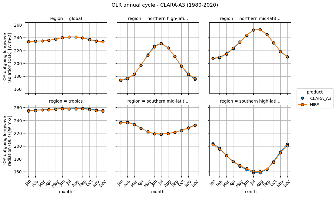
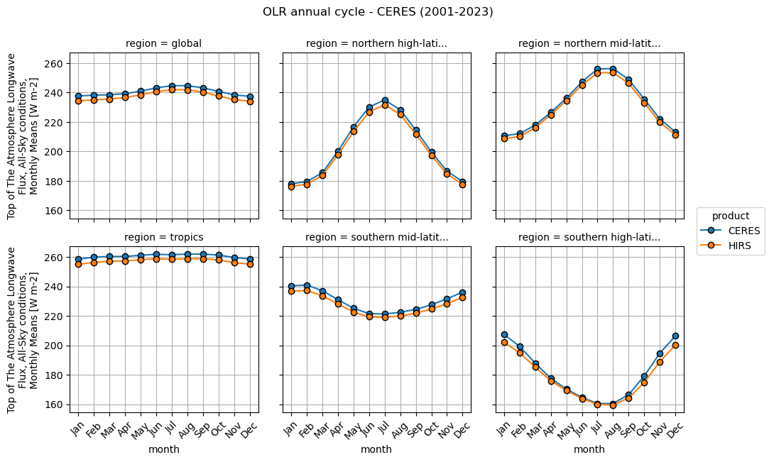
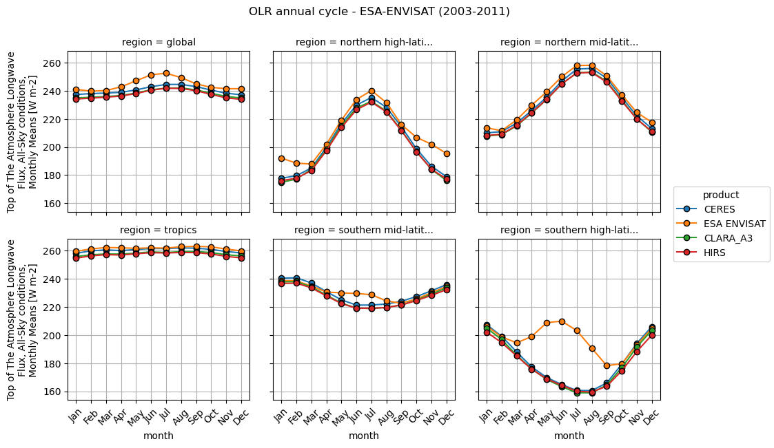
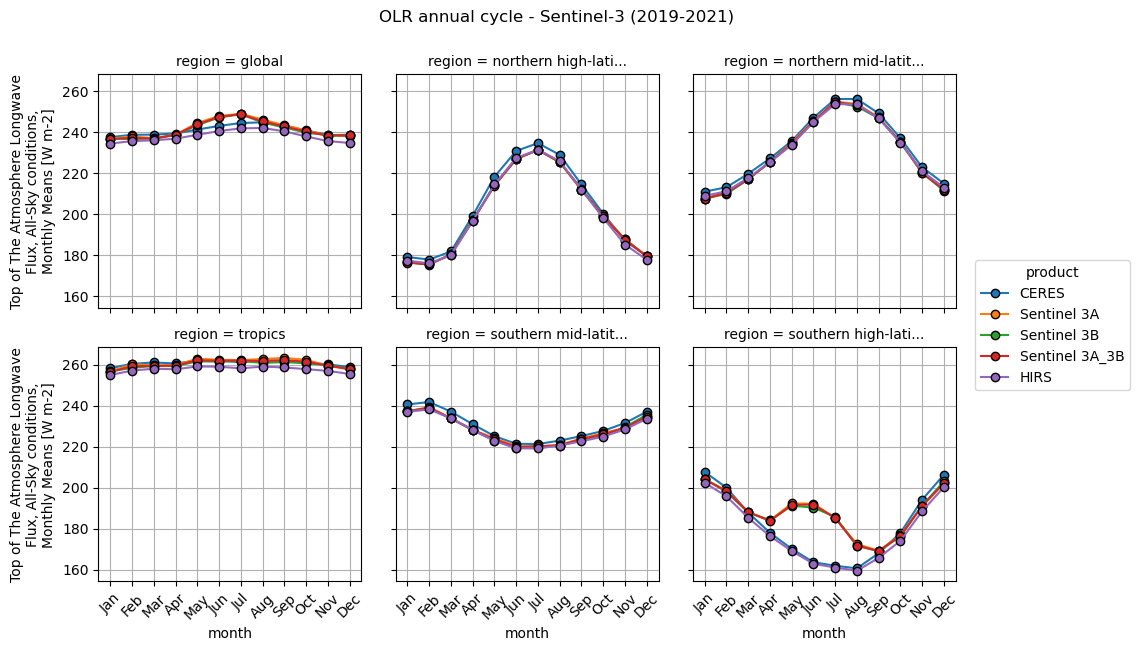
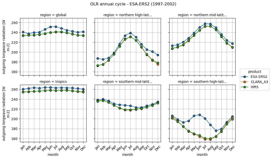
Differences in the annual cycle amplitude across datasets partly reflect data quality and sampling effects rather than purely physical variability. Overall, there is a high degree of agreement among CERES, CLARA-A3 and HIRS across all regions, with respect to what is observed when considering also ERS-2, ENVISAT and Sentinel products. These latter seem to have systematically higher climatological OLR values during hemispheric wintertime in both the northern and southern high-latitude regions, due to a seasonally varying masking of these regions. In ENVISAT, this effect is amplified by the fact that, due to its relatively reduced swath width, there is an extreme latitudinalband which is never sampled by measurements (see also the zonal mean analysis section). Despite the global region presenting typical biased values against CLARA-A3, HIRS and CERES, which are in agreement with the dataset documentation (see the ERB CCI -ICDR: Product Quality Assurance Report (PQAR)). There is no documentation available to search for further details necessary to explain Southern Hemisphere differences in ESA products (ENVISAT, Sentinel) - see section 4 of the ERB CCI-ICDR: Product Quality Assurance Document (PQAD).

Show code cell source

Hide code cell source

for label, start, stop in periods_info:
    plot_period_climatology(sw_ts_periods[label], label, start, stop, "OSR annual cycle")

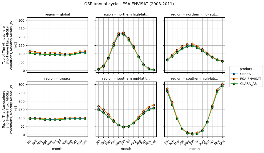
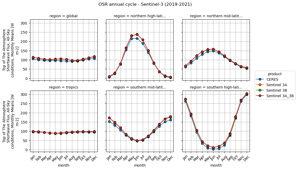
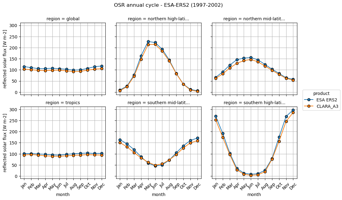
Discrepancies among OSR products are generally smaller than for OLR, reflecting the stronger observational constraint provided by reflected solar radiation. Nevertheless, differences increase poleward and over bright surfaces, consistent with known sensitivities of shortwave flux retrievals to cloud optical properties, surface albedo, and anisotropy corrections. Products derived from AATSR (ERS-2, Sentinel, ENVISAT) sensors tend to exhibit slightly higher OSR in bright subtropical and high‐latitude regions than AVHRR-based ones (CERES, CLARA-A3), in line with their documented validation characteristics ([3], [7]; [8]).

In the following cell, we define the function to build anomalies by subtracting from each dataset its climatology over the full-coverage period.

Show code cell source

Hide code cell source

def build_anomalies(ts_all):
    if ts_all is None or ts_all.sizes.get('product', 0) == 0:
        return None
    anom_list = []
    for product in ts_all.product.values:
        ts_product = ts_all.sel(product=product, drop=True).dropna("time", how="all")
        if ts_product.time.size == 0:
            continue
        climatology = ts_product.groupby("time.month").mean("time", skipna=True)
        anom = (ts_product.groupby("time.month") - climatology)
        anom_list.append(anom.expand_dims(product=[product]))
    if len(anom_list) == 0:
        return None
    return xr.concat(anom_list, dim="product")


lw_anom = build_anomalies(lw_ts)
sw_anom = build_anomalies(sw_ts)

And here we scatter-plot anomalies showing month by month variability, colour-coding the years, over different regions

Show code cell source

Hide code cell source

lw_anom = lw_anom.assign_coords(product=lw_anom.product.astype('str'), region=lw_anom.region.astype('str'))
sw_anom = sw_anom.assign_coords(product=sw_anom.product.astype('str'), region=sw_anom.region.astype('str'))

Show code cell source

Hide code cell source

if lw_anom is not None:
    for r in range(len(lw_anom.region)):
        reg_lw = lw_anom.isel(region=r)
        reg_lw = reg_lw.assign_coords({'year': reg_lw.time.dt.year})

        t4 = reg_lw.plot.scatter(
            x='month',
            col='product',
            col_wrap=4,
            hue='year',
            edgecolor='k',
            cmap='jet',
            figsize=(12, 6)
        )

        # Apply formatting to all facet axes
        for ax in t4.axes.flat:
            ax.grid()
            ax.set_xticks([1, 2, 3, 4, 5, 6, 7, 8, 9, 10, 11, 12])
            ax.set_xticklabels(['Jan', 'Feb', 'Mar', 'Apr', 'May', 'Jun', 'Jul', 'Aug', 'Sep', 'Oct', 'Nov', 'Dec'], rotation=45)
            ax.tick_params(axis="x", labelrotation=45)

        # Add global title
        t4.fig.suptitle(
            f"OLR monthly anomalies (period climatology removed) "
            f"in region {lw_anom.region.values[r]}",
            y=1.05
        )

        plt.show()

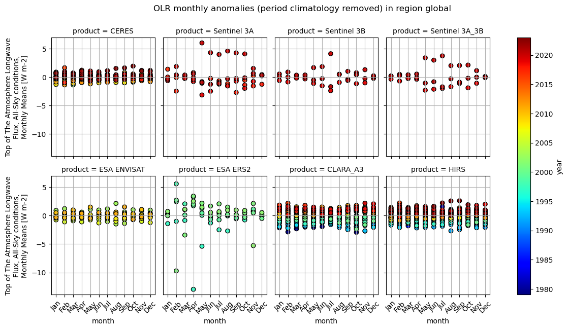
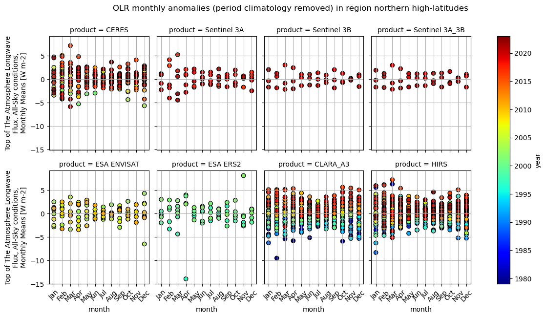
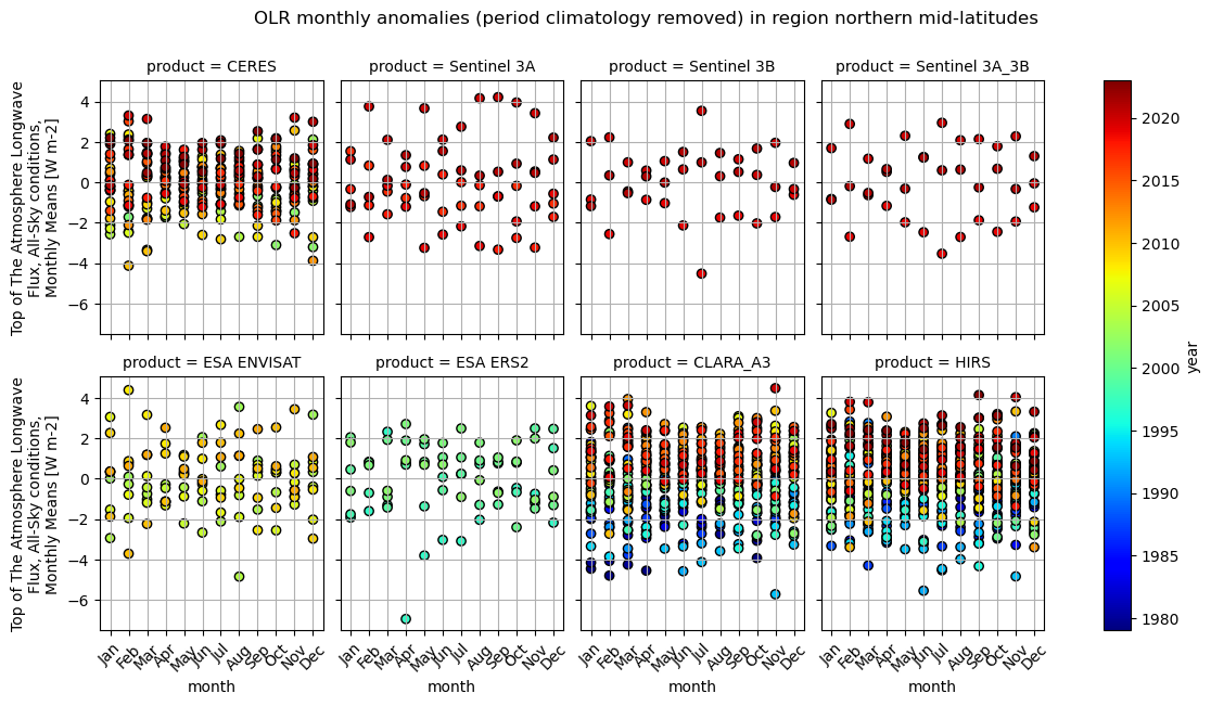
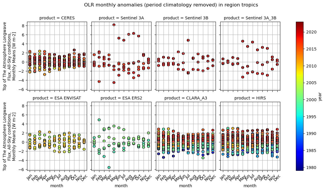
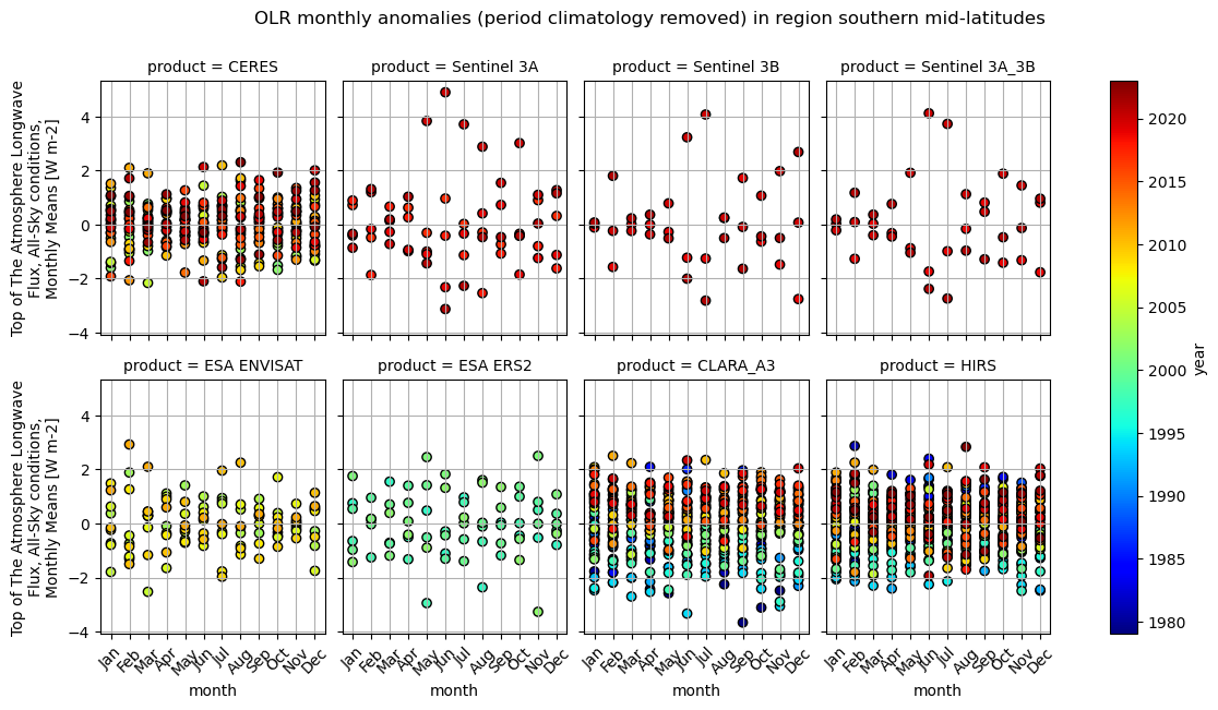
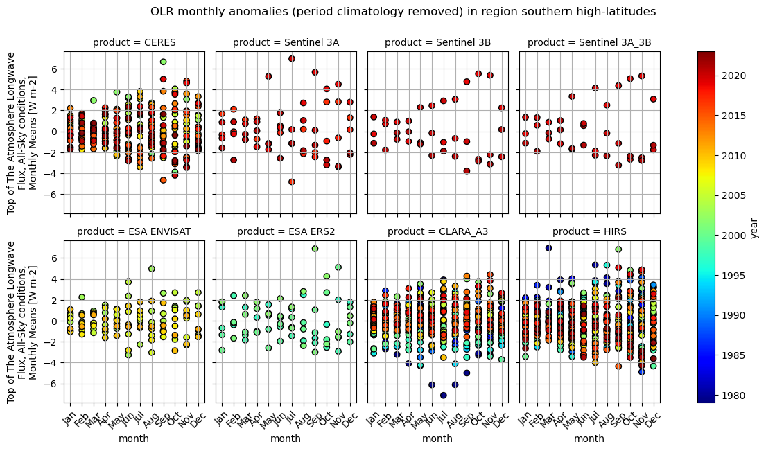
The anomaly scatter plots show that Sentinel products, ERS-2 and ENVISAT have a higher degree of variability than longer records such as CLARA-A3, CERES and HIRS. Furthermore, it appears evident from the year colour-coding that there’s a general increasing trend in the OLR, which is more pronounced in the northern regions than in the southern ones, which have reflections in globally-averaged values.

Same as above, but for the shortwave.

Show code cell source

Hide code cell source

if sw_anom is not None:
    for r in range(len(lw_anom.region)):
        reg_sw = sw_anom.isel(region=r)
        reg_sw = reg_sw.assign_coords({'year': reg_sw.time.dt.year})

        t5 = reg_sw.plot.scatter(
            x='month',
            col='product',
            col_wrap=4,
            hue='year',
            edgecolor='k',
            cmap='jet',
            figsize=(12, 6)
        )

        # Apply formatting to all facet axes
        for ax in t5.axes.flat:
            ax.grid()
            ax.set_xticks([1, 2, 3, 4, 5, 6, 7, 8, 9, 10, 11, 12])
            ax.set_xticklabels(['Jan', 'Feb', 'Mar', 'Apr', 'May', 'Jun', 'Jul', 'Aug', 'Sep', 'Oct', 'Nov', 'Dec'], rotation=45)
            ax.tick_params(axis="x", labelrotation=45)

        # Add global title
        t5.fig.suptitle(
            f"OSR monthly anomalies (period climatology removed) "
            f"in region {lw_anom.region.values[r]}",
            y=1.05
        )

        plt.show()

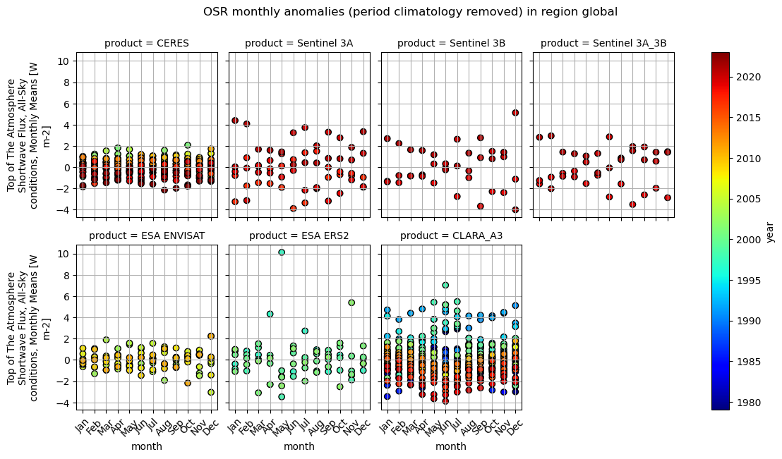
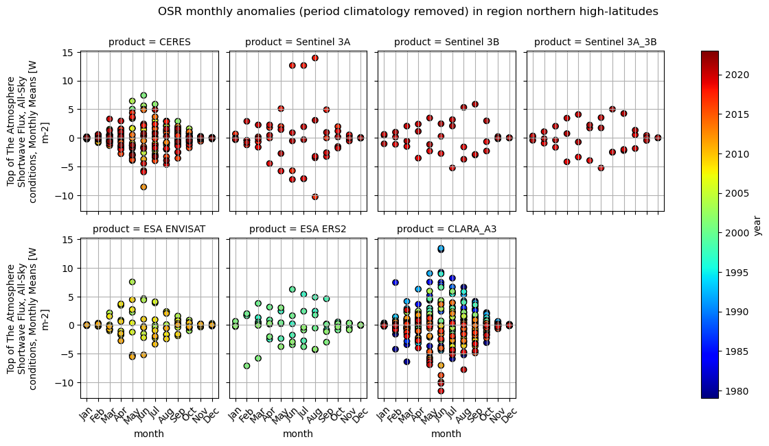
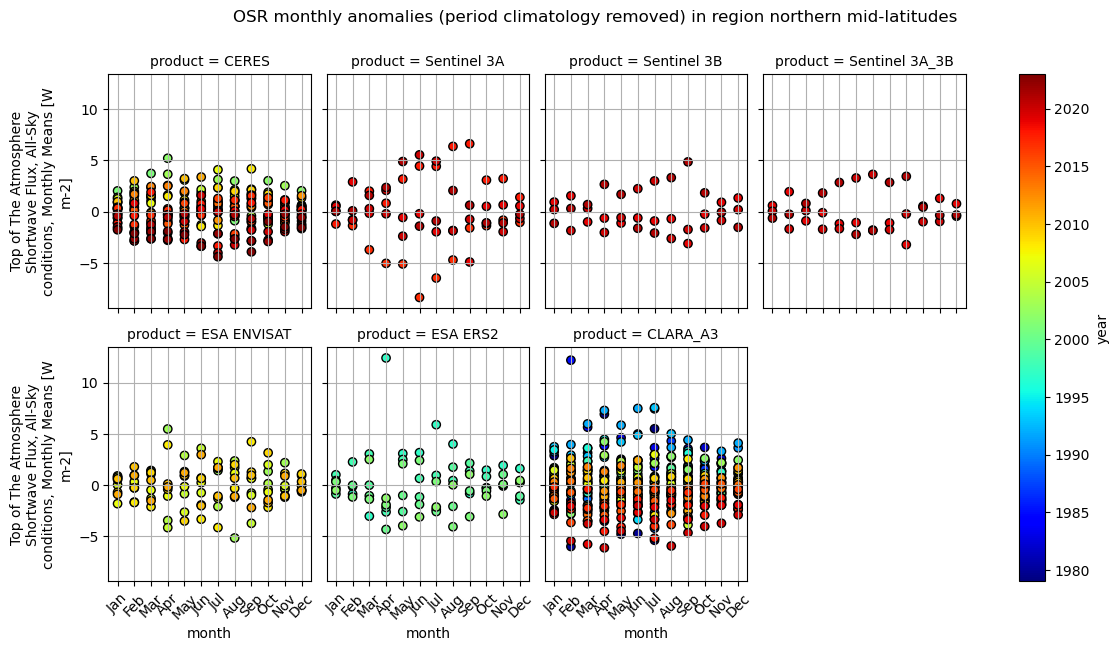
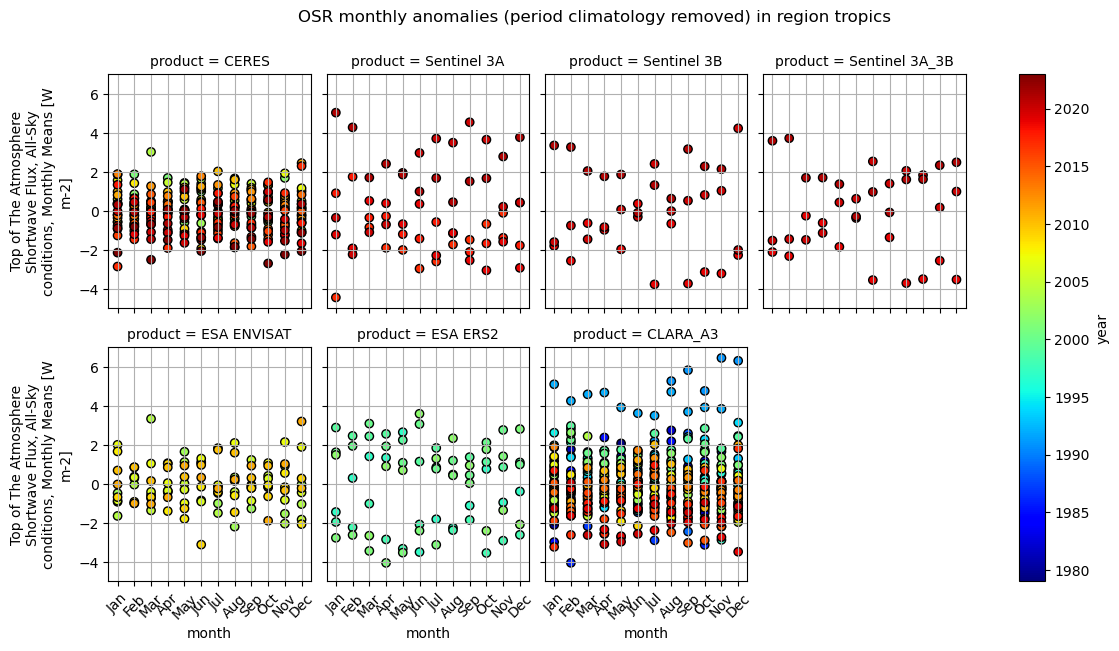
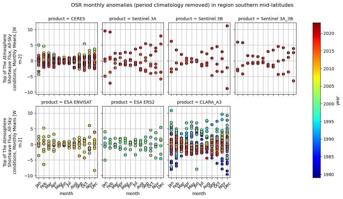
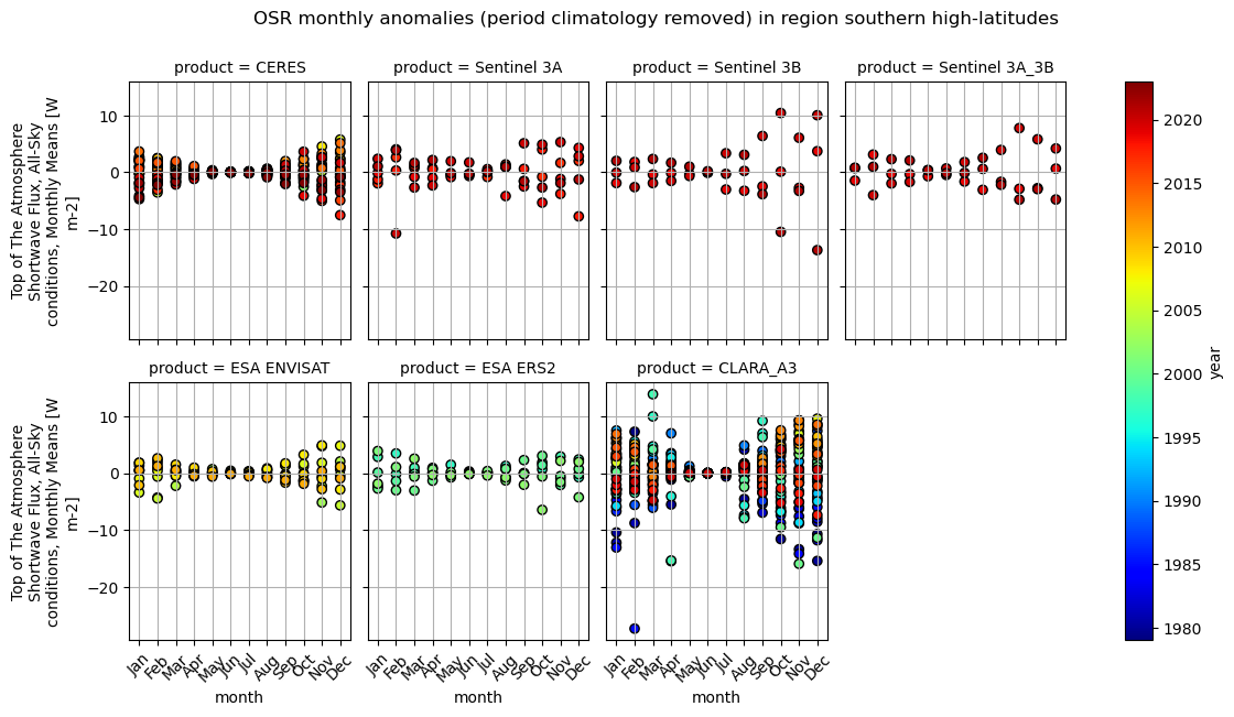
OSR anomaly scatter plots exhibit larger relative spread across products than OLR, reflecting the stronger sensitivity of reflected shortwave radiation to cloud and aerosols’ optical properties, surface radiative properties, and observation/illumination geometry. The temporal variability, even for the longest records, is characterised by a stationary behaviour, without signs of increasing or decreasing trends, nor in latitudinal bands, nor globally. For datasets with limited temporal extent, anomalies may be dominated by the particular seasonal and cloud regimes sampled during the available years, leading, also here, to representativeness limitations rather than systematic retrieval errors. Inter‐product differences in OSR anomalies should be interpreted with caution, particularly when comparing short records against multi‐decadal references such as CERES‐EBAF ([3], [7]; [8]).

Below, we calculate the Net Top of the Atmosphere Radiation, which is the unclosed “Earth Energy Imbalance” (EEI), due to missing data.

Show code cell source

Hide code cell source

p_nohirs = sw_ts.product.values
res_var = {}

p  = [r for r in request_dicts[0].keys() if r != "HIRS"]

prod = {}
for product in p:
    if product == "HIRS":
        continue
    lw_ds_complete = DS['outgoing_longwave'][product]
    sw_ds_complete = DS['outgoing_shortwave'][product]
    sw_ds_in_complete = DS['incoming_shortwave']['CERES']
    if product != "CERES":
        sw_ds_complete = diagnostics.regrid(sw_ds_complete, sw_ds_in_complete, method='bilinear')
        lw_ds_complete = diagnostics.regrid(lw_ds_complete, sw_ds_in_complete, method='bilinear')
    lw_ds = lw_ds_complete#.groupby('time.month').mean('time', skipna=True)
    sw_ds = sw_ds_complete#.groupby('time.month').mean('time', skipna=True)
    sw_ds_in = sw_ds_in_complete#.groupby('time.month').mean('time', skipna=True)
    sw_ds_in = fix_lon_0_360(sw_ds_in)
    lw_ds = fix_lon_0_360(lw_ds)
    sw_ds = fix_lon_0_360(sw_ds)
    sw_ds_in = fix_time(sw_ds_in)
    sw_ds = fix_time(sw_ds)
    lw_ds = fix_time(lw_ds)
    shortname_out = get_varname(sw_ds, 'outgoing_shortwave')
    longname = get_varname(lw_ds, 'outgoing_longwave')
    shortname_in = get_varname(sw_ds_in, 'incoming_shortwave')
    da = np.abs(sw_ds[shortname_out]) - np.abs(sw_ds_in[shortname_in]) + np.abs(lw_ds[longname])
    da = fix_time(da)
    mask_da = da.mean('time', skipna=True)
    dataarrays = []
    for region, slices in region_slices.items():
        dall = {}
        dall.update(slices)
        da_sel = da.sel(longitude=dall['lon_slice'], latitude=dall['lat_slice'])
        mask_sel = mask_da.sel(longitude=dall['lon_slice'], latitude=dall['lat_slice'])
        da_sel = da_sel.where(~np.isnan(mask_sel))
        da_ts = da_sel.weighted(np.cos(da_sel.latitude * np.pi / 180.)).mean(['longitude', 'latitude'], skipna=True)
        dataarrays.append(da_ts.expand_dims(region=[region]))
    
    da_reg = xr.concat(dataarrays, "region")
    prod[product] = da_reg
    res_var['EEI'] = prod

CERES is used here as a reference for incoming shortwave radiation and as a benchmark for Net Top Of the Atmosphere Radiation, consistent with its design objective of achieving TOA energy balance within uncertainty ([1], [4]). Specifically, NTOAR is calculated for each of the datasets in this notebook as the difference between the net shortwave and net longwave components, but the net shortwave is always calculated using the incoming component from CERES-EBAF.

Show code cell source

Hide code cell source

ensmean = xr.concat([res_var['EEI'][p] for p in p], dim='product').assign_coords({'product': p}).mean('product')
ensstd = xr.concat([res_var['EEI'][p] for p in p], dim='product').assign_coords({'product': p}).std('product')
res = xr.concat([res_var['EEI'][p] for p in p], dim='product').assign_coords({'product': p})
res = xr.concat([res, ensmean.expand_dims(product=['EnsMean'])], dim='product')

And here we show the time series for the ensemble mean and for each member, alongside the ensemble standard deviation as a grey shading. This is done in every one of the regions defined in previous analyses. The EEI is the small difference between the sunlight the Earth absorbs and the thermal (longwave) plus reflected (shortwave) radiation it emits, and represents a fundamental “engine” of climate change. Even a tiny positive imbalance (on the order of 0.5-1 W m^-2, according to recent estimates [6]) sustained year after year is what drives ocean heat uptake, ice melt, sea-level rise and ultimately the global temperature increase.

Show code cell source

Hide code cell source

for j in range(len(res.region)):
    figure = plt.figure(j, figsize=(12, 5))
    ax = figure.add_subplot(1, 1, 1)
    for i in range(len(res.product)):
        if res.product[i].values == 'EnsMean':
            continue
        res.isel(product=i).isel(region=j).plot(ax=ax, label=res.product[i].values, alpha=0.8)
    t3 = res.isel(region=j).sel(product='EnsMean').plot(ax=ax, color='k', label='EnsMean') #.resample(time='1M').mean()
    ylabel = (
    "Net\n"
    "Top Of the Atmosphere\n"
    r"Radiation = $\langle (sw_{\mathrm{out}} - sw_{\mathrm{in}}^{[\mathrm{CERES}]}) - lw \rangle$"
    "\n[W m$^{-2}$]"
    )
    ax.fill_between(ensmean.time.values,
                    (ensmean - ensstd).isel(region=j).values,
                    (ensmean + ensstd).isel(region=j).values,
                    color='gray', alpha=0.3, label='Ens. Std. Dev.')
    ax.set_ylabel(ylabel)
    ax.grid()
    ax.set_title('')
    ax.legend(loc='upper center', ncols=6, bbox_to_anchor=(0.5, 1.15))
    figure.suptitle(f"NTOAR Time series - {res.region[j].values}", y=1.05)
    plt.show()

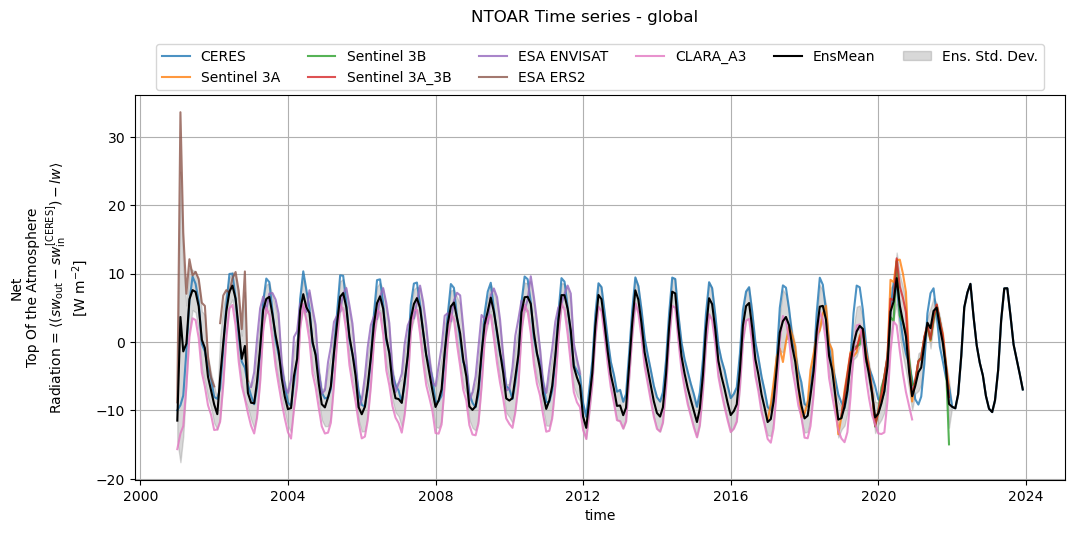
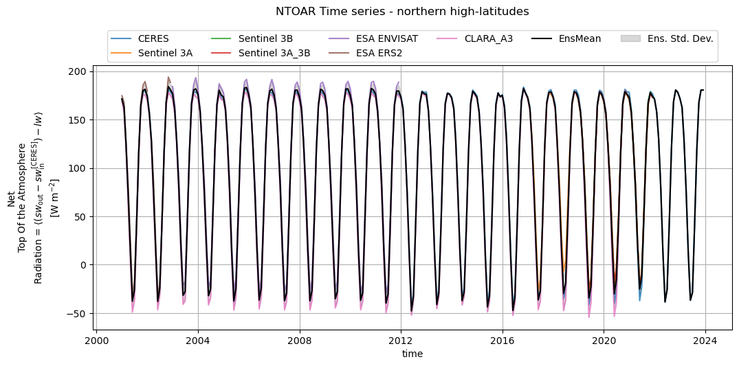
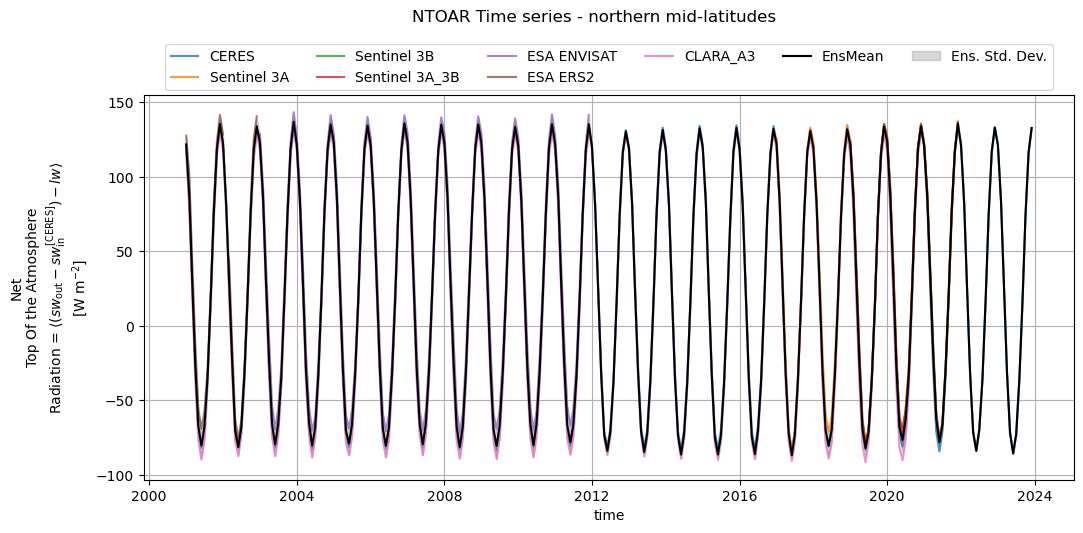
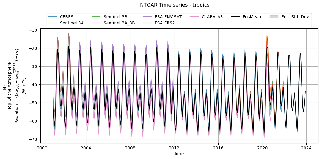
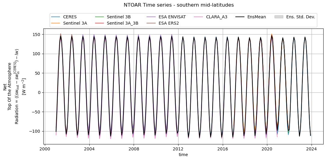
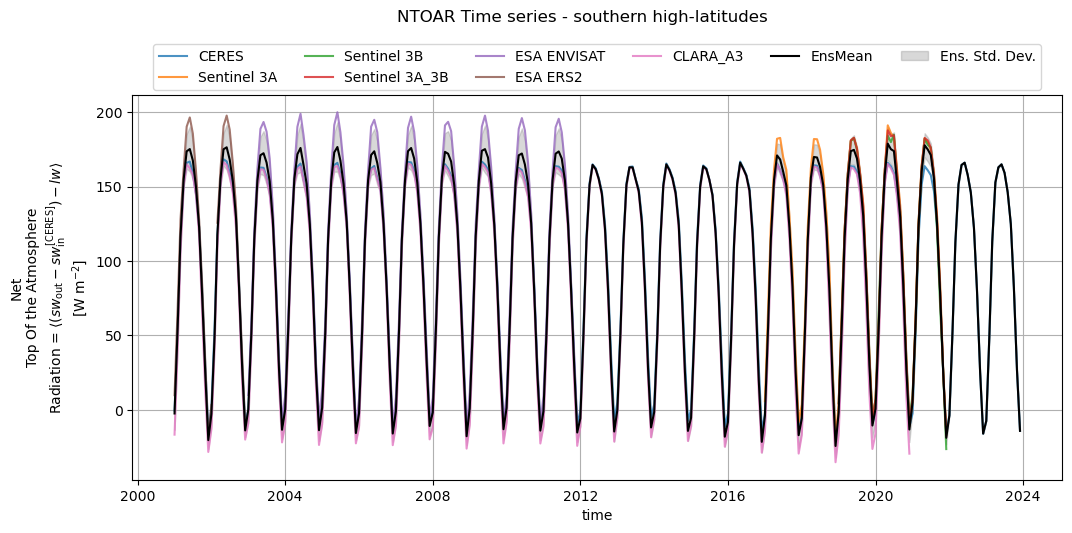
The globally averaged time series of monthly mean Net Top of the Atmosphere Radiation (NTOAR) presents two main high-variability temporal spikes: the ERS-2 one at the beginning of the time series, and another peak in 2020, clearly due to Sentinel data. The first one can be explained by the switch of the Near Infra Red channel onboard of NOAA satellites (from 3.7 to 1.6 micrometres), which changed the type of available information: the 1.6 channel allows for a better distinction between different types of clouds (ice or water). Water clouds absorb less radiation compared to ice clouds, and assuming overestimation with respect to ice clouds with the 3.7 channel, this may explain the jump, see the PVIR. The second feature is due to a known bias of sentinel products in both components (about 6 W m^-2 for the OLR, and about 4 W m^-2 for the OSR - see this PQAR). Outlier peaks apart, the global average of NTOAR indicates a small seasonal cycle (about 20 W m^-2 peak-to-peak), oscillating around zero. The tropical domain is characterised by a range of variability entirely negative, correctly indicating that on average, this is the region of net radiation gain, while mid-latitudes and high-latitudes are respectively almost in balance and losing radiation.

4. Plot time weighted means

Below, we calculate and plot time-weighted means for the different radiation budget products, with their proper masking. The dataset in each left column is taken as a reference; it is shown with its absolute values, while the others are shown as differences with respect to this one. Please note that different periods were considered in order to make a fair comparison between products which have a different temporal extent.

Show code cell source

Hide code cell source

def plot_maps_with_reference(da_all, ref_product, title, levels_abs, cmap_abs, label_abs):
    products = list(da_all.product.values)
    if ref_product not in products:
        return
    ref = da_all.sel(product=ref_product)
    other_products = [p for p in products if p != ref_product]
    if len(other_products) == 0:
        return
    anomalies = da_all.sel(product=other_products) - ref
    plot_arrays = [ref] + [anomalies.sel(product=p) for p in other_products]
    titles = [ref_product] + [f"{p} - {ref_product}" for p in other_products]
    n = len(plot_arrays)
    ncols = 2
    nrows = int(np.ceil(n / ncols))
    fig, axs = plt.subplots(
        nrows, ncols, figsize=(6 * ncols, 4 * nrows), subplot_kw={'projection': ccrs.PlateCarree(central_longitude=180)}
    )
    axs = np.array(axs).reshape(-1)
    im_abs = None
    im_diff = None
    diff_limit = 15 if "OLR" in title else 35
    for i, (da_i, t_i) in enumerate(zip(plot_arrays, titles)):
        ax = axs[i]
        if i == 0:
            im_abs = da_i.plot(
                ax=ax,
                transform=ccrs.PlateCarree(),
                cmap=cmap_abs,
                levels=levels_abs,
                extend="both",
                add_colorbar=False,
            )
            ax.set_title(f"{t_i}, range=({da_i.min().values:.1f}, {da_i.max().values:.1f})")
        else:
            im_diff = da_i.plot(
                ax=ax,
                transform=ccrs.PlateCarree(),
                cmap='coolwarm',
                vmin=-diff_limit,
                vmax=diff_limit,
                extend="both",
                add_colorbar=False,
            )
        ax.coastlines('50m')
        ax.gridlines()
        ax.set_title(f"{t_i}, range=({da_i.min().values:.1f}, {da_i.max().values:.1f})")
    for j in range(i + 1, len(axs)):
        fig.delaxes(axs[j])
    fig.set_layout_engine("compressed")
    if im_abs is not None:
        cax_abs = fig.add_axes([1.02, 0.55, 0.02, 0.35])
        fig.colorbar(im_abs, cax=cax_abs, orientation='vertical', label=label_abs)
    if im_diff is not None:
        cax_diff = fig.add_axes([1.02, 0.1, 0.02, 0.35])
        fig.colorbar(im_diff, cax=cax_diff, orientation='vertical', label=f"Bias [W m-2]")
    fig.suptitle(title)

for i, (ds_maps, times) in enumerate(zip(ds_periods_list, periods)):
    mask_period = masks_periods[i] if i < len(masks_periods) else None
    p_to_show = []
    for k in ds_maps['outgoing_longwave'].keys():
        p_to_show.append(k)

    p_to_show_whirs = p_to_show.copy()
    if "HIRS" in p_to_show_whirs:
        p_to_show_whirs = p_to_show_whirs
    if "HIRS" in p_to_show:
        p_to_show.remove("HIRS")
    lw_maps = xr.concat([ds_maps['outgoing_longwave'][p] for p in p_to_show_whirs], dim='product').assign_coords({'product': p_to_show_whirs})
    if mask_period is not None and "outgoing_longwave" in mask_period.variable.values:
        lw_maps_masked = lw_maps.where(~np.isnan(mask_period.sel(variable='outgoing_longwave')))
    else:
        lw_maps_masked = lw_maps
    if len(p_to_show_whirs) > 0:
        ref_lw = p_to_show_whirs[0]
        plot_maps_with_reference(
            lw_maps_masked,
            ref_product=ref_lw,
            title=f"Mean map on the period {times[0].year}-{times[-1].year} (OLR)",
            levels_abs=range(150, 315, 5),
            cmap_abs="nipy_spectral",
            label_abs=r"longwave [W m-2]",
        )
    if len(p_to_show) > 0:
        sw_maps = xr.concat([ds_maps['outgoing_shortwave'][p] for p in p_to_show], dim='product').assign_coords({'product': p_to_show})
        if mask_period is not None and "outgoing_shortwave" in mask_period.variable.values:
            sw_maps_masked = sw_maps.where(~np.isnan(mask_period.sel(variable='outgoing_shortwave')))
        else:
            sw_maps_masked = sw_maps
        ref_sw = p_to_show[0]
        plot_maps_with_reference(
            sw_maps_masked,
            ref_product=ref_sw,
            title=f"Mean map on the period {times[0].year}-{times[-1].year} (OSR)",
            levels_abs=range(80, 210, 5),
            cmap_abs="gist_ncar",
            label_abs=r"net shortwave [W m-2]",
        )

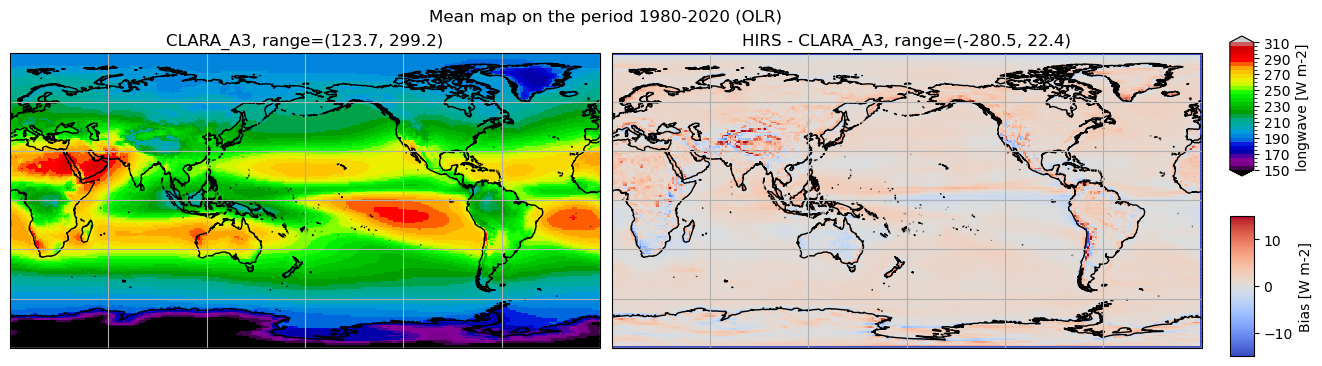
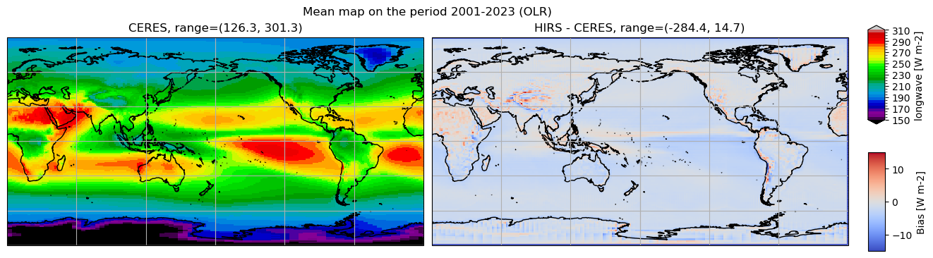
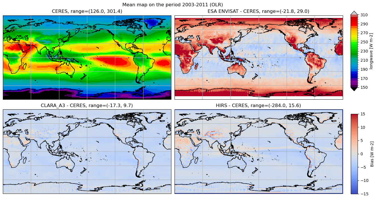
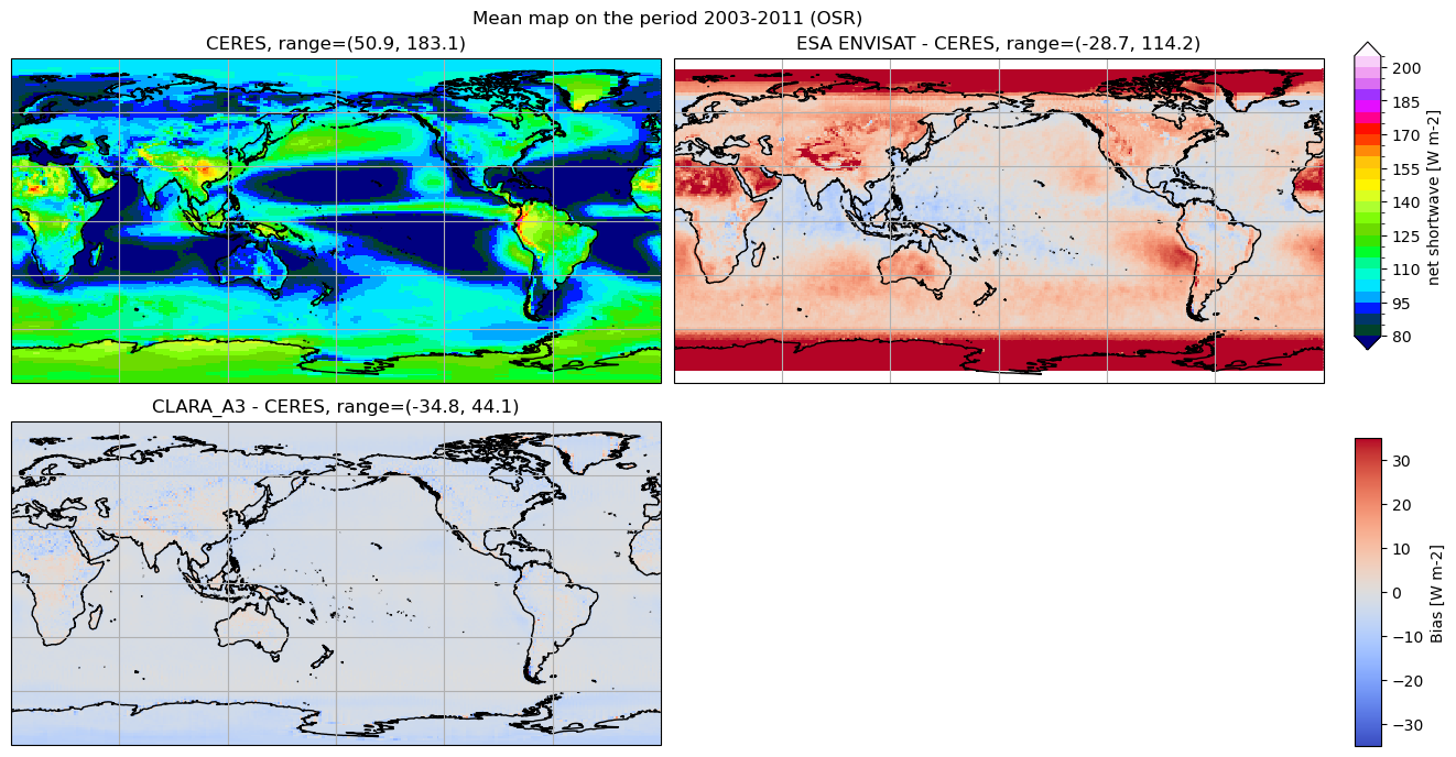
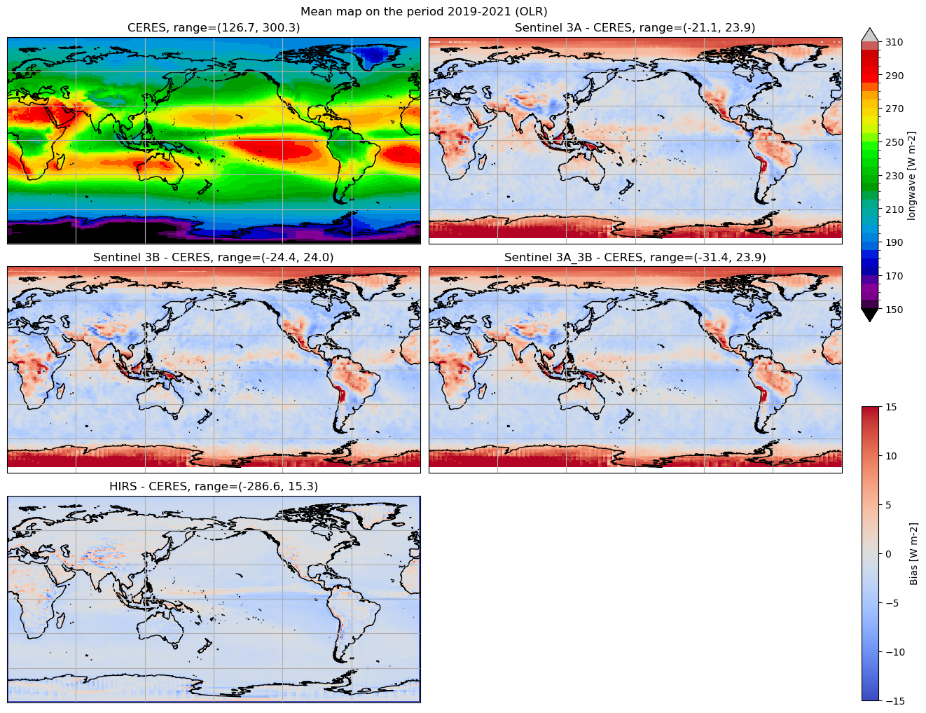
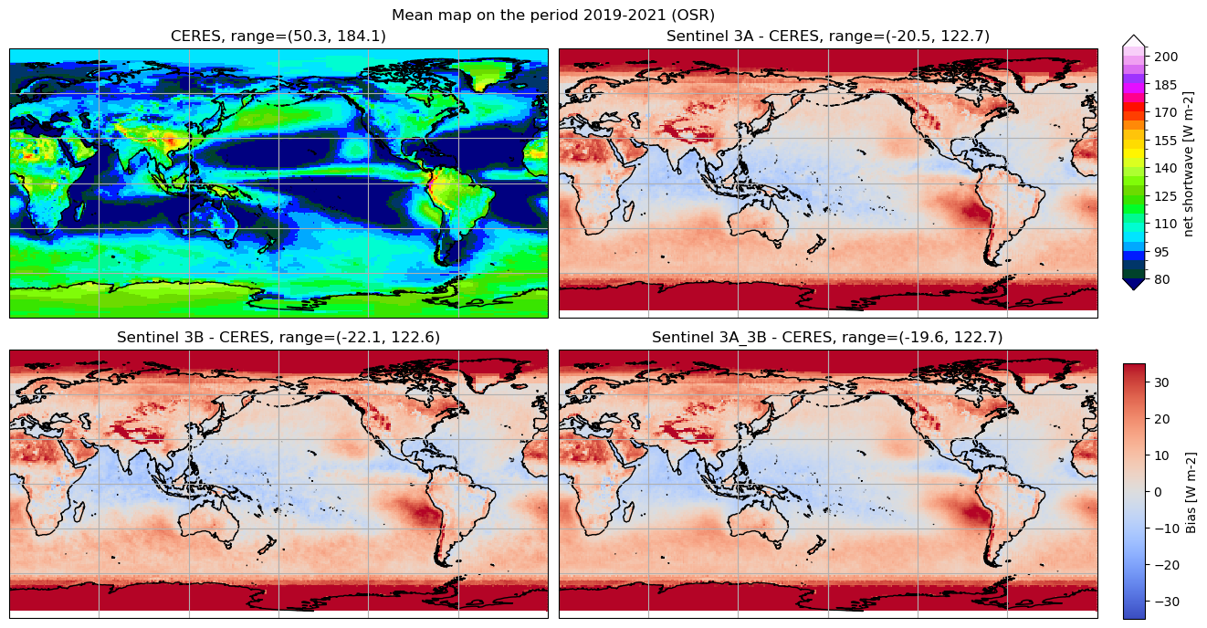
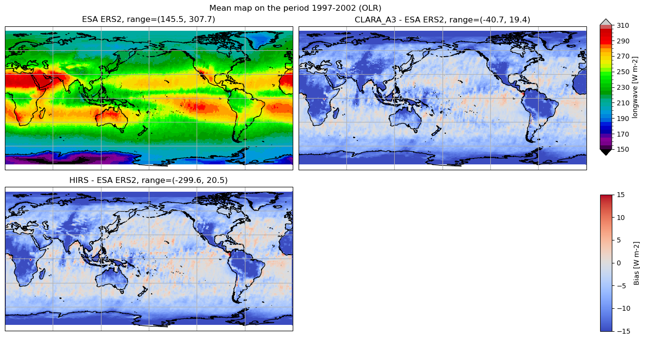
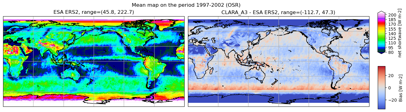
Time-averaged spatial maps show a higher degree of consistency among CLARA-A3, CERES and HIRS, which have lower bias worldwide than Sentinel, ERS-2 and ENVISAT. Common features among the bias maps are, especially for the OLR, higher values over mountain areas such as the Tibetan Plateau and the North American continent, and over desert areas, such as south of the Sahara and the Atacama, while the OSR shows a pronounced anomaly in the Tropical Pacific, offshore Chile. Maps where CERES is referenced against ERS-2, ENVISAT and Sentinel show a stripe-like pattern, especially in polar regions, which is probably due to the different types of orbit of the satellite (heliosynchronous or precessing orbit).

5. Plot spatial weighted zonal means

The code below calculates and plots weighted zonal means for the radiation budget products. For comparison, different periods are shown consistently with different temporal overlapping windows.

Show code cell source

Hide code cell source

def monthly_zonal_climatology(da, mask_common, regrid, ds_obj):
    if regrid:
        da = diagnostics.regrid(da, ds_obj, method='bilinear')
    if mask_common is not None:
        da = da.where(~np.isnan(mask_common))
    da = diagnostics.spatial_weighted_mean(da, dim="longitude", skipna=True)
    return da.groupby("time.month").mean("time", skipna=True)

period_bounds = [
    ("CLARA-A3", clara_a3_start, clara_a3_end),
    ("CERES", ceres_start, ceres_end),
    ("ESA-ENVISAT", esa_envisat_start, esa_envisat_end),
    ("Sentinel-3", sentinel_start, sentinel_end),
    ("ESA-ERS2", esa_ers2_start, esa_ers2_end),
 ]
zonal_clim = {}

for label, start, stop in period_bounds:
    for variable in ["outgoing_longwave", "outgoing_shortwave"]:
        clim_list = []
        products_plot = []
        if "CERES" not in DS[variable]:
            continue
        ref_varname = get_varname(DS[variable]["CERES"], variable)
        da_obj = DS[variable]["CERES"][ref_varname]
        for product, ds in DS[variable].items():
            if product == "HIRS" and variable != "outgoing_longwave":
                continue
            if "CERES" not in product and variable == "incoming_shortwave":
                continue
            prod_start = start_var[variable][product]
            prod_stop = stop_var[variable][product]
            curr_time = pd.date_range(prod_start, prod_stop)
            period_time = pd.date_range(start, stop)
            if period_time[0] not in curr_time or period_time[-1] not in curr_time:
                continue
            varname = get_varname(ds, variable)
            da = ds[varname].sel(time=slice(start, stop))
            regrid = False if product == "CERES" else True
            mask_common = get_period_mask(label, variable)
            clim = monthly_zonal_climatology(da, mask_common, regrid, da_obj)
            clim_list.append(clim.expand_dims(product=[product]))
            products_plot.append(product)
        if len(clim_list) == 0:
            continue
        clim_all = xr.concat(clim_list, dim="product").assign_coords({"product": products_plot})
        if len(products_plot) <= 1:
            continue
        zonal_clim[(variable, label)] = clim_all

The results are shown in an Hovmoller plot, with the latitude on the y-axis and the month on the x-axis. As for the mean maps, the first panel in each column is in absolute value, while the others show the bias relative to the first.

Show code cell source

Hide code cell source

for label, start, stop in period_bounds:
    for variable in ["outgoing_longwave", "outgoing_shortwave"]:
        clim_all = zonal_clim.get((variable, label))
        if clim_all is None:
            continue
        #t = clim_all.plot(col="month", y="latitude", hue="product", col_wrap=6, figsize=(15, 7))
        #for n, ax in enumerate(t.axs.flatten()):
        #    ax.grid()
        #    ax.set_xlabel(f"{variable} [W m-2]")
        #    if n < 6:
        #        ax.set_xlabel('')
        #    ax.set_ylim(-90,90)
        #t.fig.suptitle(f"Monthly climatological zonal mean ({label} {start[:4]}-{stop[:4]}) - {variable}", y=1.02)
        products = list(clim_all.product.values)
        if not products:
            continue
        ref_product = products[0]
        ref = clim_all.sel(product=ref_product)
        n = len(products)
        ncols = 2
        nrows = int(np.ceil(n / ncols))
        fig, axs = plt.subplots(nrows, ncols, figsize=(10, 5 * nrows), squeeze=False)
        axs = axs.flatten()
        im_abs = None
        im_diff = None
        diff_limit = 10 if variable=='outgoing_longwave' else 25
        for i, p in enumerate(products):
            ax = axs[i]
            if i == 0:
                im_abs = ref.plot(
                    ax=ax,
                    x="month",
                    y="latitude",
                    cmap="turbo",
                    add_colorbar=False,
                )
                ax.set_title(f"{p}, range=({ref.min().values:.2f}, {ref.max().values:.2f})")
            else:
                diff = clim_all.sel(product=p) - ref
                im_diff = diff.plot(
                    ax=ax,
                    x="month",
                    y="latitude",
                    cmap="coolwarm",
                    add_colorbar=False,
                    vmin=-diff_limit,
                    vmax=diff_limit,
                )
                ax.set_title(f"{p} - {ref_product}, range=({diff.min().values:.2f}, {diff.max().values:.2f})")
                ax.grid()
                ax.set_ylim(-90, 90)
                ax.set_xticks([1, 2, 3, 4, 5, 6, 7, 8, 9, 10, 11, 12])
                ax.set_xticklabels(['Jan','Feb','Mar','Apr','May','Jun','Jul','Aug','Sep','Oct','Nov','Dec'])
                ax.set_ylabel("Lat [degrees]" if i % ncols == 0 else "")
                ax.set_xlabel("Month" if i >= (nrows - 1) * ncols else "")
        for j in range(n, len(axs)):
            fig.delaxes(axs[j])
        fig.set_layout_engine("compressed")
        if im_abs is not None:
            cax_abs = fig.add_axes([1.02, 0.55, 0.02, 0.35])
            fig.colorbar(im_abs, cax=cax_abs, orientation="vertical", label=f"{variable} [W m-2]")
        if im_diff is not None:
            cax_diff = fig.add_axes([1.02, 0.1, 0.02, 0.35])
            fig.colorbar(im_diff, cax=cax_diff, orientation="vertical", label="Bias [W m-2]")
        fig.suptitle(
            f"Monthly climatological zonal mean ({label} {start[:4]}-{stop[:4]}) - {variable}",
            y=1.05,
        )

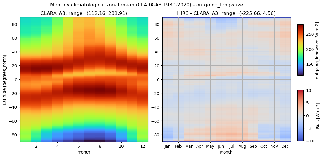
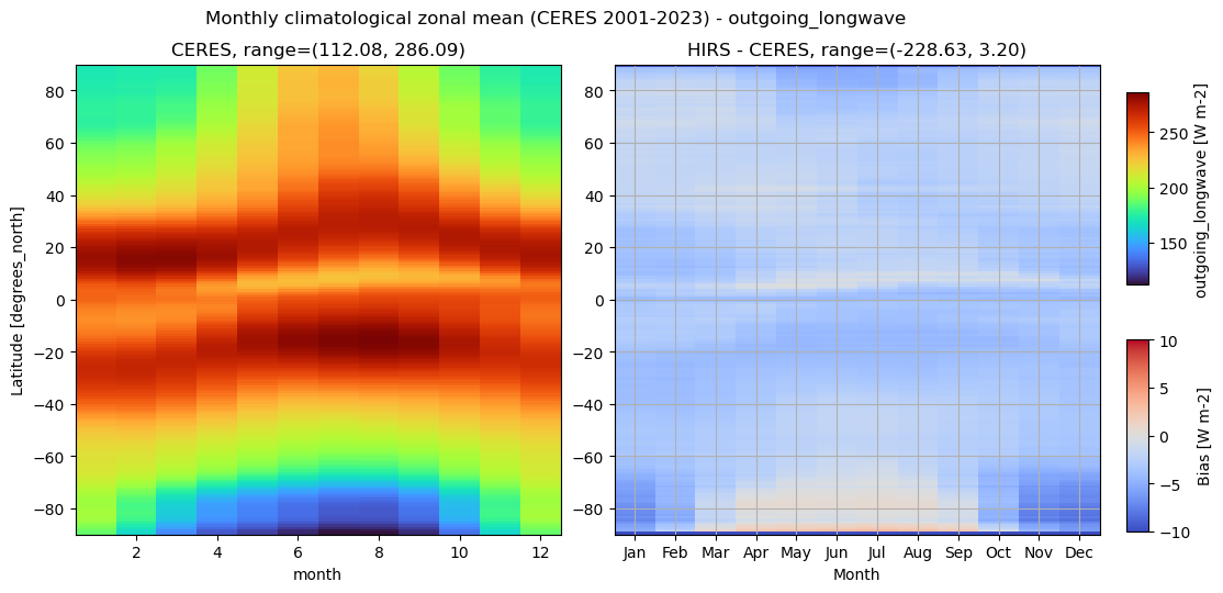
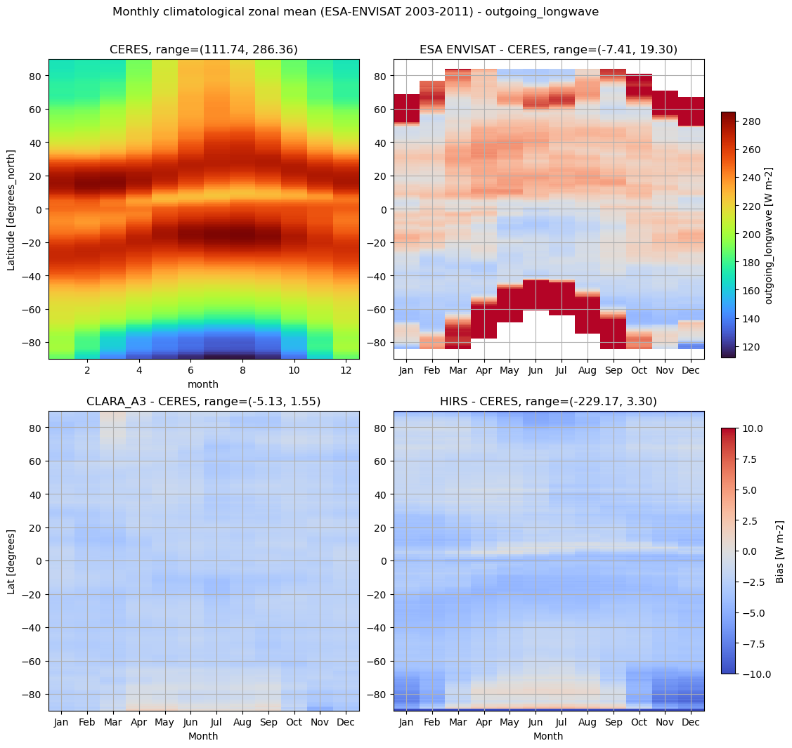
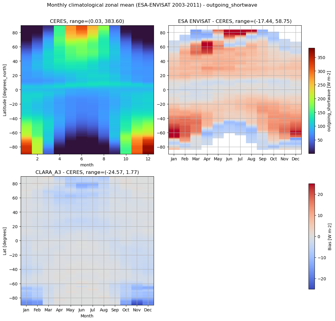
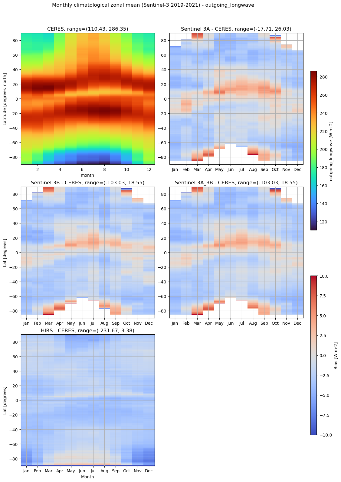
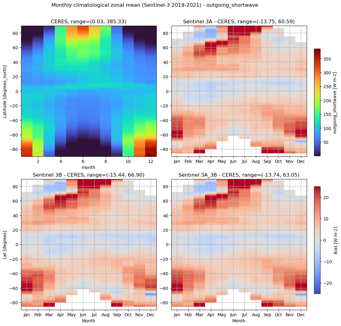
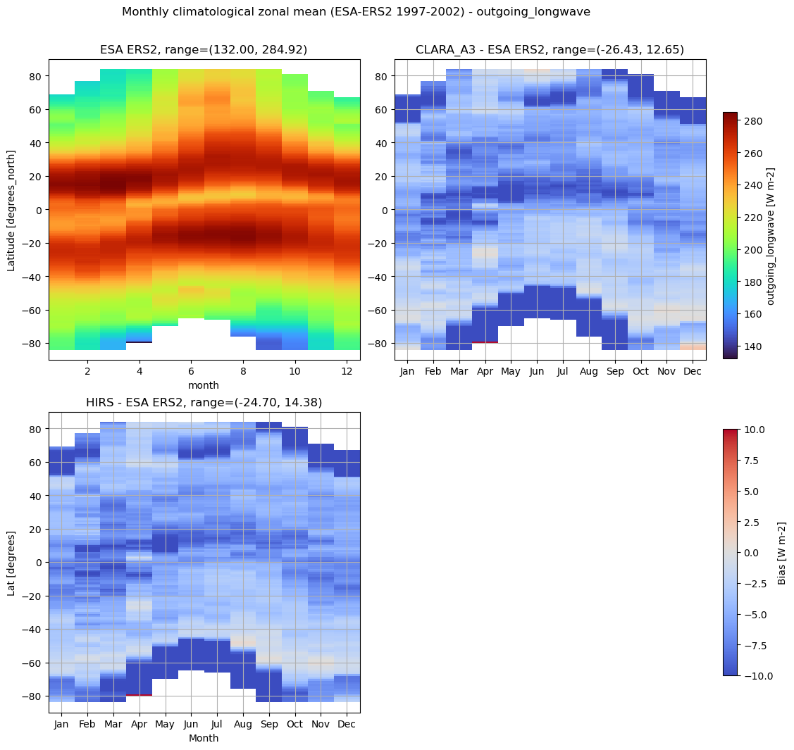
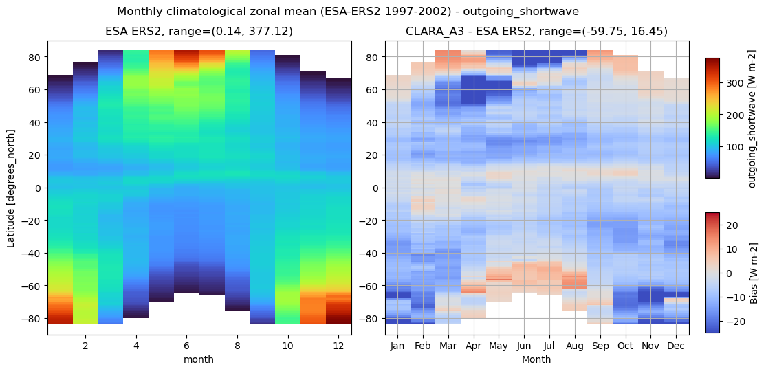
Zonal averages indicate consistency on main climatological features among the products, with systematic deviations emerging poleward (e.g., south of 50°S and north of 50°N). These discrepancies are consistent with increased uncertainty in cloud detection and classification, surface characterisation, and anisotropy corrections at high latitudes, particularly for products not specifically optimised for TOA flux closure. Remarkable differences in OLR zonal means persist with ERS-2, ENVISAT, and Sentinel products. Take, for example, the comparison of the CERES dataset with the ESA‑ENVISAT, CLARA‑A3, and HIRS datasets. As described in Section 4 of the Cloud_cci ATBD v6.2, differences in sampling density, sensor spectral capabilities, and the non‑linear aggregation of pixel‑level fluxes play a central role in shaping these biases. The ERS-2/ENVISAT/Sentinel products in general show moderate, latitude‑dependent deviations from the dataset chosen as reference, reflecting the limited sampling of AATSR and SLSTR sensors, and the sensitivity of broadband fluxes to cloud‑top retrieval uncertainties. CLARA‑A3 exhibits small and spatially smooth differences, consistent with the dense AVHRR sampling and the stability of its Level‑3 processing chain. In contrast, the larger HIRS‑CERES discrepancies highlight the impact of coarse spatial resolution and differing radiative assumptions. Together, these diagnostics reinforce the interpretation that high‑latitude biases arise from a combination of algorithmic and sampling factors inherent to the various sensor systems ([3], [5]).

Discussion and applications

The differences identified across the OLR and OSR datasets primarily reflect known characteristics of the satellite instruments and retrieval algorithms used to construct the various climate data records. For OLR, the spread between the CERES EBAF record and the HIRS and CLARA-A3 products is consistent with the long-recognised sensitivity of longwave flux retrievals to spectral sampling, cloud detection, and scene-dependent angular corrections ([1], [3], [5]). CERES derives broadband fluxes using detailed angular-distribution models (ADMs) developed specifically for top-of-atmosphere applications [2]. In contrast, HIRS and the AVHRR-based CLARA-A3 rely on narrower channels and empirical regressions to estimate broadband longwave radiation, a known source of latitudinal and surface-type–dependent discrepancies documented in their validation reports (HIRS PVR, CLARA-A3 PVR). These differences help explain the stronger gradients observed in the CLARA-A3 OLR fields and the slight warm-scene bias in HIRS over subtropical dry regions.

Additional spatial structures visible in the ERS-2 (ATSR-2/AATSR) maps, when compared with CLARA-A3, manifest as track-like or striping features that do not correspond to known geophysical patterns. These features are consistent with sampling artefacts related to the narrow swath width and orbit characteristics of the ATSR-2 instrument. ATSR-2 provides high radiometric accuracy and dual-view observations but samples the Earth with a relatively narrow swath, resulting in sparse spatial coverage when averaged over limited time periods. In the absence of extensive gap-filling, this can leave residual orbit‐related traces in climatological and bias maps. In contrast, the AVHRR instruments underlying CLARA-A3 have a much wider swath and denser spatial sampling, which tends to smooth out such sampling artefacts when forming long-term means, despite their more limited angular information. The presence of these traces should therefore be interpreted as a representativeness and sampling limitation rather than as a systematic bias in the radiative flux retrievals. Similar sampling‐related features in narrow‐swath ERB products have been documented in previous intercomparisons and validation studies ([2], [3], [8]).

The Sentinel-3 SLSTR (3A, 3B, and the merged 3A+3B) interim CDRs show overall good consistency with the CERES reference but display enhanced variability in the tropics and over land surfaces, likely due to the spectral characteristics of the sensors (atmospheric windows), and their consequent high-sensitivity to the reconstruction of the diurnal cycle. However, this behaviour is in line with their validation documentation, which highlights sensitivity to cloud screening and to the limited temporal extent of the interim SLSTR record relative to multi-decadal products (CERES Quality Summary, Sentinel Quality Assurance Document). The relatively short data period (2017–2021) also means that interannual variability associated with ENSO events — known to modulate tropical OLR [9] — can disproportionately influence the mean differences when compared to long records such as CERES or HIRS.

For OSR, discrepancies among products similarly reflect differences in sensor spectral coverage, calibration stability in the visible and near-infrared, and the treatment of anisotropy in the shortwave domain. CERES shortwave fluxes benefit from scene-dependent ADMs and long-term calibration stability [1], [3], [4], which contribute to the coherent latitudinal reflection patterns typically used as a benchmark. The CLARA-A3 product, derived from AVHRR, shows slightly higher reflected shortwave radiation in bright subtropical and high-latitude regions, consistent with known limitations in AVHRR-based angular corrections and cloud-phase retrievals noted in its product validation reports. Similarly, OSR from ESA’s ENVISAT AATSR and from SLSTR shows small but systematic differences over marine stratocumulus regions—areas where shortwave anisotropy and cloud optical properties strongly influence flux retrievals. These patterns are consistent with prior evaluations of shortwave absorption and model–observation differences [7], [8].

Overall, the magnitude and spatial structure of the inter-product differences observed here align with previously documented behaviour of broadband radiation datasets and with theoretical expectations derived from radiative-transfer and climate-feedback studies [10], [11], [12], [6]. The consistency of many features across independent retrievals—particularly the subtropical shortwave reflection maxima and the tropical longwave minima—supports the robustness of these products for climatological analyses, while the remaining discrepancies can be traced to well-understood algorithmic and instrumental differences identified in the respective validation reports.

ℹ️ If you want to know more

Key resources

Code libraries used:

• C3S EQC custom functions, c3s_eqc_automatic_quality_control, prepared by B-Open

• CERES (Clouds and the Earth’s Radiant Energy System) CERES-EBAF product documentation, algorithm theoretical basis documents (ATBDs), and data quality summaries provide detailed descriptions of broadband flux retrievals, angular-distribution models, calibration, and uncertainty estimates. CERES Page

• NOAA HIRS OLR Climate Data Record Product and validation reports describing the construction of the HIRS OLR CDR, including spectral regression methods, sampling limitations, and known sources of uncertainty. HIRS Page

• CLARA-A3 (Cloud, Albedo and Radiation Dataset) Comprehensive documentation on AVHRR-based radiation and cloud products, including sampling characteristics, limitations at high latitudes, and validation results. CM SAF Page

• ESA Cloud Climate Change Initiative (Cloud_cci) Algorithm descriptions and product validation reports for ATSR-2, AATSR, and SLSTR-based cloud and radiation products, with emphasis on swath geometry and cloud property retrievals. ESA CCI Page

• C3S global energy balance and Earth Energy Imbalance indicators Background material explaining how ERB products are used within C3S to support climate indicators and assessments. Climate Indicators

• Tutorial on the Earth Radiation Budget (ERB) Essential Climate Variable

References

[1] Loeb, N. G., Wielicki, B. A., Doelling, D. R., Smith, G. L., Keyes, D. F., Kato, S., … & Wong, T. (2009). Toward optimal closure of the Earth’s top-of-atmosphere radiation budget. Journal of Climate, 22(3), 748-766 https://doi.org/10.1175/2008JCLI2637.1

[2] Wielicki, B. A., Barkstrom, B. R., Harrison, E. F., Lee III, R. B., Smith, G. L., & Cooper, J. E. (1996). Clouds and the Earth’s Radiant Energy System (CERES): An Earth observing system experiment. Bulletin of the American Meteorological Society, 77(5), 853-868. https://doi.org/10.1175/1520-0477(1996)077<0853:CATERE>2.0.CO;2

[3] Loeb, N. G., Wielicki, B. A., Su, W., Loukachine, K., Sun, W., Wong, T., … & Lin, B. (2012). Advances in understanding top-of-atmosphere radiation variability from satellite observations. Surveys in Geophysics, 33(3-4), 359-385 https://doi.org/10.1007/s10712-012-9175-1

[4] Loeb, N. G., J. M. Lyman, G. C. Johnson, R. P. Allan, D. R. Doelling, T. Wong, B. J. Soden, and G. L. Stephens, 2012: Observed changes in top-of-the-atmosphere radiation and upper-ocean heating consistent within uncertainty. Nat. Geosci., 5, 110–113, https://doi.org/10.1038/ngeo1375

[5] Susskind, J., G. Molnar, L. Iredell, et al., 2012: Interannual variability of outgoing longwave radiation as observed by AIRS and CERES. J. Geophys. Res. Atmos., 117, D23107, https://doi.org/10.1029/2012JD017997

[6] von Schuckmann, K. and Coauthors, 2023: Heat stored in the Earth system 1960–2020: where does the energy go? Earth System Science Data, 15(4), 1675-1709, https://doi.org/10.5194/essd-15-1675-2023

[7] Schwarz, M., D. Folini, S. Yang, and M. Wild, 2019: The Annual Cycle of Fractional Atmospheric Shortwave Absorption in Observations and Models: Spatial Structure, Magnitude, and Timing. J. Climate, 32, 6729–6748, https://doi.org/10.1175/JCLI-D-19-0212.1

[8] Yang, S., Zhang, X., Guan, S., Zhao, W., Duan, Y., Yao, Y., … Jiang, B. (2023). A review and comparison of surface incident shortwave radiation from multiple data sources: satellite retrievals, reanalysis data and GCM simulations. International Journal of Digital Earth, 16(1), 1332–1357. https://doi.org/10.1080/17538947.2023.2198262

[9] Su, W., N. G. Loeb, L. Liang, N. Liu, and C. Liu (2017), The El Niño–Southern Oscillation effect on tropical outgoing longwave radiation: A daytime versus nighttime perspective, J. Geophys. Res. Atmos., 122, 7820–7833, https://doi.org/10.1002/2017JD027002

[10] Donohoe, A., Armour, K. C., Pendergrass, A. G., & Battisti, D. S. (2014). Shortwave and longwave radiative contributions to global warming under increasing CO2. Proceedings of the National Academy of Sciences, 111(47), 16700-16705. https://doi.org/10.1073/pnas.1412190111

[11] Soden, B. J., and I. M. Held, 2006: An Assessment of Climate Feedbacks in Coupled Ocean–Atmosphere Models. J. Climate, 19, 3354–3360, https://doi.org/10.1175/JCLI3799.1

[12] von Schuckmann, K., and Coauthors, 2016: An imperative to monitor Earth’s energy balance. Nat. Climate Change, 6, 138–144, https://doi.org/10.1038/nclimate2876