

2.1. In-situ precipitation completeness for climate monitoring#
Production date: 21/10/2024
Produced by: Ana Oliveira and Luís Figueiredo (CoLAB +ATLANTIC)
🌍 Use case: Assessment of Climate Change.#
❓ Quality assessment question#
User Question: How consistent is the 30-year precipitation climatology over time? How consistent are precipitation trends from E-OBS compared to those from reanalysis products?
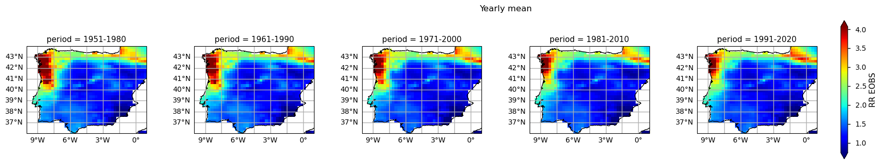
In this Use Case, we will access the E-OBS daily gridded meteorological data for Europe from 1950 to present derived from in-situ observations (henceforth, E-OBS) data from the Climate Data Store (CDS) of the Copernicus Climate Change Service (C3S) and analyse the spatial consistency of the E-OBS precipitation (RR) climatology, and its ensemble, over a given Area of Interest (AoI), as a regional example of using E-OBS in the scope of the European State of Climate [1]. The analysis includes:
(i) the climatology and probability density function of each alternative 30-year period available (i.e., 1951-1980, 1961-1990, 1971-2000, 1981-2010, 1991-2020);
(ii) the linear trends of the annual amount of days when precipitation ≥ 10mm, as defined by the World Meteorological Organization’s Expert Team on Sector-Specific Climate Indices (ET-SCI) in conjunction with sector experts [2] and following the World Meteorological Organization (WMO) standards [3];
(iii) the corresponding maps, to disclose where RR extremes are changing the most.
📢 Quality assessment statement#
These are the key outcomes of this assessment
Daily precipitation (RR) from E-OBS offers complete temporal-spatial coverage over the AoI, showing significative inter-annual variability and non-significant trends, consistent with ERA5 and those reported in the literature [4].
According to [5], both E-OBS and ERA5 demonstrate accuracy in capturing precipitation patterns, with E-OBS showing good agreement in regions with dense station networks, while ERA5 exhibits consistent mesoscale pattern representation.
According to previous authors [6] [7] who studied the consistency of precipitation values depicted in E-OBS and compared it to 2 additional datasets (ERA5 and CMORPH) over Europe, E-OBS has superior reliability in regions with dense data.
Both authors thus concluded that E-OBS captures extreme values of precipitation in areas with high data density, but may smooth out extreme events in data-sparse regions. Hence, since the input stations are not fully available, the ensemble spread should be used as a complementary indicator of the confidence level and variability of such data.
📋 Methodology#
1. Define the AoI, search and download E-OBS
2. Plot the climatology and the probability density function (PDF) for alternative 30-year periods
3. Calculate and plot seasonal PDFs and the climatological season maps
4. Calculate the annual count of days
5. Main takeaways
📈 Analysis and results#
1. Define the AoI, search and download E-OBS#
Import all the libraries/packages#
We will be working with data in NetCDF format. To best handle this data we will use libraries for working with multidimensional arrays, in particular Xarray. We will also need libraries for plotting and viewing data, in this case we will use Matplotlib and Cartopy.
Show code cell source
import matplotlib.pyplot as plt
import numpy as np
import pandas as pd
import pymannkendall as mk
import scipy.stats
import xarray as xr
from c3s_eqc_automatic_quality_control import diagnostics, download, plot

plt.style.use("seaborn-v0_8-notebook")
Data Overview#
To search for data, visit the CDS website: http://cds.climate.copernicus.eu. Here you can search for ‘in-situ observations’ using the search bar. The data we need for this tutorial is the E-OBS daily gridded meteorological data for Europe from 1950 to present derived from in-situ observations. This catalogue entry provides a daily gridded dataset of historical meteorological observations, covering Europe (land-only), from 1950 to the present. This data is derived from in-situ meteorological stations, made available through the European Climate Assessment & Dataset (ECA&D) project, as provided by National Meteorological and Hydrological Services (NMHSs) and other data-holding institutes.
E-OBS comprises a set of spatially continuous Essential Climate Variables (ECVs) from the Surface Atmosphere, following the Global Climate Observing System (GCOS) convention, provided as the mean and spread of the spatial prediction ensemble algorithm, at regular latitude-longitude grid intervals (at a 0.1° and 0.25° spatial resolution), and covering a long time-period, from 1 January 1950 to present-day. In addition to the land surface elevation, E-OBS includes daily air temperature (mean, maximum and minimum), precipitation amount, wind speed, sea-level pressure and shortwave downwelling radiation.
The E-OBS version used for this Use Case, E-OBSv28.0e, was released in October 2023 and its main difference from the previous E-OBSv27.0e is the inclusion of new series and some corrections for precipitation stations.
Having selected the correct dataset, we now need to specify what product type, variables, temporal and geographic coverage we are interested in. In this Use Case, the ensemble mean of precipitation (RR) will be used, considering the last version available (v28.0e). These can all be selected in the “Download data” tab from the CDS. In this tab a form appears in which we will select the following parameters to download, for example:
Product Type: Ensemble mean
Variable: daily precipitation sum
Grid resolution: 0.25
Period: Full period
Version: 28.0e
Format: Zip file (.zip)
At the end of the download form, select Show API request. This will reveal a block of code, which you can simply copy and paste into a cell of your Jupyter Notebook …
1.1. Download and prepare E-OBS data#
… having copied the API request to a Jupyter Notebook cell, running it will retrieve and download the data you requested into your local directory. However, before you run it, the terms and conditions of this particular dataset need to have been accepted directly at the CDS website. The option to view and accept these conditions is given at the end of the download form, just above the Show API request option. In addition, it is also useful to define the time period and AoI parameters and edit the request accordingly, as exemplified in the cells below.
Show code cell source
# Define climatology periods - ToI
years_start = [1951, 1961, 1971, 1981, 1991]
years_stop = [1980, 1990, 2000, 2010, 2020]
colors = ["deepskyblue", "green", "gold", "darkorange", "red"]
assert len(years_start) == len(years_stop) == len(colors)

# Define region of interest - AoI
area = [44, -10, 36, 1]  # N, W, S, E
assert len(area) == 4
Show code cell source
# Define request
collection_id = "insitu-gridded-observations-europe"
request = {
    "variable": ["precipitation_amount"],
    "grid_resolution": "0_25deg",
    "period": "full_period",
    "version": ["30_0e"],
    "area": area,
}

collection_id_era5 = "reanalysis-era5-single-levels"
request_era5 = {
    "product_type": ["ensemble_mean"],
    "variable": ["total_precipitation"],
    "time": [f"{hour:02d}:00" for hour in range(0, 24, 3)],
    "area": area,
}
start = f"{min(years_start)}-01"
stop = f"{max(years_stop)}-12"
request_era5 = download.update_request_date(request_era5, start, stop)
Show code cell source
# Define transform function to reduce downloaded data
def dayofyear_reindex(ds, years_start, years_stop):
    # 15-day rolling mean
    ds_rolled = ds.rolling(time=15, center=True).mean()

    # Extract periods
    datasets = []
    for year_start, year_stop in zip(years_start, years_stop):
        period = f"{year_start}-{year_stop}"
        ds_masked = ds_rolled.where(
            (ds_rolled["time"].dt.year >= year_start)
            & (ds_rolled["time"].dt.year <= year_stop),
            drop=True,
        )
        datasets.append(
            ds_masked.groupby("time.dayofyear").mean().expand_dims(period=[period])
        )
    ds_dayofyear = xr.merge(datasets)

    # Add season (pick any leap year)
    season = xr.DataArray(
        pd.to_datetime(ds_dayofyear["dayofyear"].values - 1, unit="D", origin="2008"),
    ).dt.season
    return ds_dayofyear.assign_coords(season=("dayofyear", season.values))

def accumulated_spatial_weighted_mean(ds):
    ds = ds.resample(time="1D").sum(keep_attrs=True)
    return diagnostics.spatial_weighted_mean(ds)
Show code cell source
# Periods
dataarrays = []
for reduction in ("mean", "spread"):
    print(f"{reduction=}")
    da = download.download_and_transform(
        collection_id,
        request | {"product_type": f"ensemble_{reduction}"},
        transform_func=dayofyear_reindex,
        transform_func_kwargs={"years_start": years_start, "years_stop": years_stop},
    )["rr"]
    dataarrays.append(da.rename(reduction))
    da.attrs["long_name"] += f" {reduction}"
ds_periods = xr.merge(dataarrays)

# Timeseries
da_eobs = download.download_and_transform(
    collection_id,
    request | {"product_type": "ensemble_mean"},
    transform_func=diagnostics.spatial_weighted_mean,
)["rr"]
da_eobs = da_eobs.sel(time=slice(start, stop))

da_era5 = download.download_and_transform(
    collection_id_era5,
    request_era5,
    backend_kwargs={"time_dims": ["valid_time"]},
    transform_func=accumulated_spatial_weighted_mean,
    chunks={"year": 1},
    n_jobs=2,
)["tp"]

da_timeseries = xr.concat(
    [
        da_eobs.expand_dims(product=["E-OBS"]),
        (da_era5 * 1.0e3).expand_dims(product=["ERA5"]),
    ],
    "product",
)
reduction='mean'
  0%|          | 0/1 [00:00<?, ?it/s]2025-04-02 16:35:46,618 INFO [2024-09-26T00:00:00] Watch our [Forum](https://forum.ecmwf.int/) for Announcements, news and other discussed topics.
2025-04-02 16:35:46,619 WARNING [2024-06-16T00:00:00] CDS API syntax is changed and some keys or parameter names may have also changed. To avoid requests failing, please use the "Show API request code" tool on the dataset Download Form to check you are using the correct syntax for your API request.
2025-04-02 16:35:46,819 INFO [2024-09-26T00:00:00] Watch our [Forum](https://forum.ecmwf.int/) for Announcements, news and other discussed topics.
2025-04-02 16:35:46,821 WARNING [2024-06-16T00:00:00] CDS API syntax is changed and some keys or parameter names may have also changed. To avoid requests failing, please use the "Show API request code" tool on the dataset Download Form to check you are using the correct syntax for your API request.
2025-04-02 16:35:47,034 INFO Request ID is e04387a4-68d7-4d43-9173-7b866e7df474
2025-04-02 16:35:47,346 INFO status has been updated to accepted
2025-04-02 16:35:52,617 INFO status has been updated to running
2025-04-02 16:38:39,841 INFO status has been updated to successful
100%|██████████| 1/1 [07:14<00:00, 434.22s/it]
reduction='spread'
  0%|          | 0/1 [00:00<?, ?it/s]2025-04-02 16:43:00,887 INFO [2024-09-26T00:00:00] Watch our [Forum](https://forum.ecmwf.int/) for Announcements, news and other discussed topics.
2025-04-02 16:43:00,889 WARNING [2024-06-16T00:00:00] CDS API syntax is changed and some keys or parameter names may have also changed. To avoid requests failing, please use the "Show API request code" tool on the dataset Download Form to check you are using the correct syntax for your API request.
2025-04-02 16:43:01,107 INFO [2024-09-26T00:00:00] Watch our [Forum](https://forum.ecmwf.int/) for Announcements, news and other discussed topics.
2025-04-02 16:43:01,110 WARNING [2024-06-16T00:00:00] CDS API syntax is changed and some keys or parameter names may have also changed. To avoid requests failing, please use the "Show API request code" tool on the dataset Download Form to check you are using the correct syntax for your API request.
2025-04-02 16:43:01,498 INFO Request ID is e58ee98d-d951-4e5d-8383-212177f1f629
2025-04-02 16:43:01,591 INFO status has been updated to accepted
2025-04-02 16:43:10,146 INFO status has been updated to running
2025-04-02 16:45:59,101 INFO status has been updated to successful
100%|██████████| 1/1 [06:24<00:00, 384.90s/it]
100%|██████████| 1/1 [01:45<00:00, 105.70s/it]
2025-04-02 16:51:15,437 INFO [2024-09-26T00:00:00] Watch our [Forum](https://forum.ecmwf.int/) for Announcements, news and other discussed topics.
2025-04-02 16:51:15,437 WARNING [2024-06-16T00:00:00] CDS API syntax is changed and some keys or parameter names may have also changed. To avoid requests failing, please use the "Show API request code" tool on the dataset Download Form to check you are using the correct syntax for your API request.
2025-04-02 16:51:15,522 INFO [2024-09-26T00:00:00] Watch our [Forum](https://forum.ecmwf.int/) for Announcements, news and other discussed topics.
2025-04-02 16:51:15,522 WARNING [2024-06-16T00:00:00] CDS API syntax is changed and some keys or parameter names may have also changed. To avoid requests failing, please use the "Show API request code" tool on the dataset Download Form to check you are using the correct syntax for your API request.
2025-04-02 16:51:15,640 INFO [2024-09-26T00:00:00] Watch our [Forum](https://forum.ecmwf.int/) for Announcements, news and other discussed topics.
2025-04-02 16:51:15,640 WARNING [2024-06-16T00:00:00] CDS API syntax is changed and some keys or parameter names may have also changed. To avoid requests failing, please use the "Show API request code" tool on the dataset Download Form to check you are using the correct syntax for your API request.
2025-04-02 16:51:15,734 INFO [2024-09-26T00:00:00] Watch our [Forum](https://forum.ecmwf.int/) for Announcements, news and other discussed topics.
2025-04-02 16:51:15,734 WARNING [2024-06-16T00:00:00] CDS API syntax is changed and some keys or parameter names may have also changed. To avoid requests failing, please use the "Show API request code" tool on the dataset Download Form to check you are using the correct syntax for your API request.
2025-04-02 16:51:16,098 INFO Request ID is 66aa4451-be06-4aba-b4e5-49451b81ada6
2025-04-02 16:51:16,133 INFO Request ID is d5eb30cb-4bf5-47de-96b5-0834cd7c5962
2025-04-02 16:51:16,177 INFO status has been updated to accepted
2025-04-02 16:51:16,228 INFO status has been updated to accepted
2025-04-02 16:51:24,663 INFO status has been updated to running
2025-04-02 16:51:29,820 INFO status has been updated to successful
2025-04-02 16:51:29,899 INFO status has been updated to successful
2025-04-02 16:51:31,975 INFO [2024-09-26T00:00:00] Watch our [Forum](https://forum.ecmwf.int/) for Announcements, news and other discussed topics.
2025-04-02 16:51:31,975 WARNING [2024-06-16T00:00:00] CDS API syntax is changed and some keys or parameter names may have also changed. To avoid requests failing, please use the "Show API request code" tool on the dataset Download Form to check you are using the correct syntax for your API request.
2025-04-02 16:51:32,186 INFO [2024-09-26T00:00:00] Watch our [Forum](https://forum.ecmwf.int/) for Announcements, news and other discussed topics.
2025-04-02 16:51:32,186 WARNING [2024-06-16T00:00:00] CDS API syntax is changed and some keys or parameter names may have also changed. To avoid requests failing, please use the "Show API request code" tool on the dataset Download Form to check you are using the correct syntax for your API request.
2025-04-02 16:51:32,300 INFO [2024-09-26T00:00:00] Watch our [Forum](https://forum.ecmwf.int/) for Announcements, news and other discussed topics.
2025-04-02 16:51:32,301 WARNING [2024-06-16T00:00:00] CDS API syntax is changed and some keys or parameter names may have also changed. To avoid requests failing, please use the "Show API request code" tool on the dataset Download Form to check you are using the correct syntax for your API request.
2025-04-02 16:51:32,514 INFO [2024-09-26T00:00:00] Watch our [Forum](https://forum.ecmwf.int/) for Announcements, news and other discussed topics.
2025-04-02 16:51:32,514 WARNING [2024-06-16T00:00:00] CDS API syntax is changed and some keys or parameter names may have also changed. To avoid requests failing, please use the "Show API request code" tool on the dataset Download Form to check you are using the correct syntax for your API request.
2025-04-02 16:51:32,565 INFO Request ID is 42bd9ca9-de59-4454-9cc1-028cf6391cbb
2025-04-02 16:51:32,641 INFO status has been updated to accepted
2025-04-02 16:51:32,917 INFO Request ID is e6d38a46-ef91-47a6-b61b-e2ee7ca3f53d
2025-04-02 16:51:32,997 INFO status has been updated to accepted
2025-04-02 16:51:37,756 INFO status has been updated to running
2025-04-02 16:51:41,208 INFO status has been updated to successful
2025-04-02 16:51:41,433 INFO status has been updated to running
2025-04-02 16:51:43,391 INFO [2024-09-26T00:00:00] Watch our [Forum](https://forum.ecmwf.int/) for Announcements, news and other discussed topics.
2025-04-02 16:51:43,391 WARNING [2024-06-16T00:00:00] CDS API syntax is changed and some keys or parameter names may have also changed. To avoid requests failing, please use the "Show API request code" tool on the dataset Download Form to check you are using the correct syntax for your API request.
2025-04-02 16:51:43,611 INFO [2024-09-26T00:00:00] Watch our [Forum](https://forum.ecmwf.int/) for Announcements, news and other discussed topics.
2025-04-02 16:51:43,611 WARNING [2024-06-16T00:00:00] CDS API syntax is changed and some keys or parameter names may have also changed. To avoid requests failing, please use the "Show API request code" tool on the dataset Download Form to check you are using the correct syntax for your API request.
2025-04-02 16:51:44,058 INFO Request ID is d452379d-096a-4bc4-8680-951268382125
2025-04-02 16:51:44,148 INFO status has been updated to accepted
2025-04-02 16:51:46,577 INFO status has been updated to successful
2025-04-02 16:51:48,701 INFO [2024-09-26T00:00:00] Watch our [Forum](https://forum.ecmwf.int/) for Announcements, news and other discussed topics.
2025-04-02 16:51:48,701 WARNING [2024-06-16T00:00:00] CDS API syntax is changed and some keys or parameter names may have also changed. To avoid requests failing, please use the "Show API request code" tool on the dataset Download Form to check you are using the correct syntax for your API request.
2025-04-02 16:51:48,903 INFO [2024-09-26T00:00:00] Watch our [Forum](https://forum.ecmwf.int/) for Announcements, news and other discussed topics.
2025-04-02 16:51:48,903 WARNING [2024-06-16T00:00:00] CDS API syntax is changed and some keys or parameter names may have also changed. To avoid requests failing, please use the "Show API request code" tool on the dataset Download Form to check you are using the correct syntax for your API request.
2025-04-02 16:51:49,271 INFO Request ID is 3cebb31d-d349-4abb-9457-291423677af5
2025-04-02 16:51:49,347 INFO status has been updated to accepted
2025-04-02 16:51:52,581 INFO status has been updated to running
2025-04-02 16:51:57,721 INFO status has been updated to successful
2025-04-02 16:51:57,774 INFO status has been updated to running
2025-04-02 16:51:59,412 INFO [2024-09-26T00:00:00] Watch our [Forum](https://forum.ecmwf.int/) for Announcements, news and other discussed topics.
2025-04-02 16:51:59,412 WARNING [2024-06-16T00:00:00] CDS API syntax is changed and some keys or parameter names may have also changed. To avoid requests failing, please use the "Show API request code" tool on the dataset Download Form to check you are using the correct syntax for your API request.
2025-04-02 16:51:59,630 INFO [2024-09-26T00:00:00] Watch our [Forum](https://forum.ecmwf.int/) for Announcements, news and other discussed topics.
2025-04-02 16:51:59,630 WARNING [2024-06-16T00:00:00] CDS API syntax is changed and some keys or parameter names may have also changed. To avoid requests failing, please use the "Show API request code" tool on the dataset Download Form to check you are using the correct syntax for your API request.
2025-04-02 16:52:00,025 INFO Request ID is a307bad7-1d5a-4775-abf0-d6599d1035ef
2025-04-02 16:52:00,097 INFO status has been updated to accepted
2025-04-02 16:52:02,915 INFO status has been updated to successful
2025-04-02 16:52:04,611 INFO [2024-09-26T00:00:00] Watch our [Forum](https://forum.ecmwf.int/) for Announcements, news and other discussed topics.
2025-04-02 16:52:04,611 WARNING [2024-06-16T00:00:00] CDS API syntax is changed and some keys or parameter names may have also changed. To avoid requests failing, please use the "Show API request code" tool on the dataset Download Form to check you are using the correct syntax for your API request.
2025-04-02 16:52:04,817 INFO [2024-09-26T00:00:00] Watch our [Forum](https://forum.ecmwf.int/) for Announcements, news and other discussed topics.
2025-04-02 16:52:04,817 WARNING [2024-06-16T00:00:00] CDS API syntax is changed and some keys or parameter names may have also changed. To avoid requests failing, please use the "Show API request code" tool on the dataset Download Form to check you are using the correct syntax for your API request.
2025-04-02 16:52:05,267 INFO Request ID is e1cfce61-7f4b-4ccb-89de-b4173bda147e
2025-04-02 16:52:05,345 INFO status has been updated to accepted
2025-04-02 16:52:08,594 INFO status has been updated to running
2025-04-02 16:52:13,741 INFO status has been updated to successful
2025-04-02 16:52:13,825 INFO status has been updated to running
2025-04-02 16:52:15,423 INFO [2024-09-26T00:00:00] Watch our [Forum](https://forum.ecmwf.int/) for Announcements, news and other discussed topics.
2025-04-02 16:52:15,423 WARNING [2024-06-16T00:00:00] CDS API syntax is changed and some keys or parameter names may have also changed. To avoid requests failing, please use the "Show API request code" tool on the dataset Download Form to check you are using the correct syntax for your API request.
2025-04-02 16:52:15,654 INFO [2024-09-26T00:00:00] Watch our [Forum](https://forum.ecmwf.int/) for Announcements, news and other discussed topics.
2025-04-02 16:52:15,655 WARNING [2024-06-16T00:00:00] CDS API syntax is changed and some keys or parameter names may have also changed. To avoid requests failing, please use the "Show API request code" tool on the dataset Download Form to check you are using the correct syntax for your API request.
2025-04-02 16:52:16,171 INFO Request ID is a9410a45-8805-4438-a984-4a98f2c19325
2025-04-02 16:52:16,270 INFO status has been updated to accepted
2025-04-02 16:52:19,044 INFO status has been updated to successful
2025-04-02 16:52:21,361 INFO [2024-09-26T00:00:00] Watch our [Forum](https://forum.ecmwf.int/) for Announcements, news and other discussed topics.
2025-04-02 16:52:21,361 WARNING [2024-06-16T00:00:00] CDS API syntax is changed and some keys or parameter names may have also changed. To avoid requests failing, please use the "Show API request code" tool on the dataset Download Form to check you are using the correct syntax for your API request.
2025-04-02 16:52:21,485 INFO status has been updated to running
2025-04-02 16:52:21,565 INFO [2024-09-26T00:00:00] Watch our [Forum](https://forum.ecmwf.int/) for Announcements, news and other discussed topics.
2025-04-02 16:52:21,565 WARNING [2024-06-16T00:00:00] CDS API syntax is changed and some keys or parameter names may have also changed. To avoid requests failing, please use the "Show API request code" tool on the dataset Download Form to check you are using the correct syntax for your API request.
2025-04-02 16:52:22,096 INFO Request ID is 31f909aa-f1e6-466e-8c47-fd95547f75b6
2025-04-02 16:52:22,172 INFO status has been updated to accepted
2025-04-02 16:52:24,954 INFO status has been updated to successful
2025-04-02 16:52:26,439 INFO [2024-09-26T00:00:00] Watch our [Forum](https://forum.ecmwf.int/) for Announcements, news and other discussed topics.
2025-04-02 16:52:26,439 WARNING [2024-06-16T00:00:00] CDS API syntax is changed and some keys or parameter names may have also changed. To avoid requests failing, please use the "Show API request code" tool on the dataset Download Form to check you are using the correct syntax for your API request.
2025-04-02 16:52:26,642 INFO [2024-09-26T00:00:00] Watch our [Forum](https://forum.ecmwf.int/) for Announcements, news and other discussed topics.
2025-04-02 16:52:26,643 WARNING [2024-06-16T00:00:00] CDS API syntax is changed and some keys or parameter names may have also changed. To avoid requests failing, please use the "Show API request code" tool on the dataset Download Form to check you are using the correct syntax for your API request.
2025-04-02 16:52:27,133 INFO Request ID is b1404de3-b60c-45d7-a14a-ca574bb16151
2025-04-02 16:52:27,211 INFO status has been updated to accepted
2025-04-02 16:52:30,611 INFO status has been updated to running
2025-04-02 16:52:35,773 INFO status has been updated to successful
2025-04-02 16:52:36,081 INFO status has been updated to running
2025-04-02 16:52:37,560 INFO [2024-09-26T00:00:00] Watch our [Forum](https://forum.ecmwf.int/) for Announcements, news and other discussed topics.
2025-04-02 16:52:37,560 WARNING [2024-06-16T00:00:00] CDS API syntax is changed and some keys or parameter names may have also changed. To avoid requests failing, please use the "Show API request code" tool on the dataset Download Form to check you are using the correct syntax for your API request.
2025-04-02 16:52:37,799 INFO [2024-09-26T00:00:00] Watch our [Forum](https://forum.ecmwf.int/) for Announcements, news and other discussed topics.
2025-04-02 16:52:37,800 WARNING [2024-06-16T00:00:00] CDS API syntax is changed and some keys or parameter names may have also changed. To avoid requests failing, please use the "Show API request code" tool on the dataset Download Form to check you are using the correct syntax for your API request.
2025-04-02 16:52:38,388 INFO Request ID is 43d5988d-7d3f-42f2-a903-f16c557cc884
2025-04-02 16:52:38,523 INFO status has been updated to accepted
2025-04-02 16:52:43,448 INFO status has been updated to successful
2025-04-02 16:52:45,741 INFO status has been updated to running
2025-04-02 16:52:45,809 INFO [2024-09-26T00:00:00] Watch our [Forum](https://forum.ecmwf.int/) for Announcements, news and other discussed topics.
2025-04-02 16:52:45,809 WARNING [2024-06-16T00:00:00] CDS API syntax is changed and some keys or parameter names may have also changed. To avoid requests failing, please use the "Show API request code" tool on the dataset Download Form to check you are using the correct syntax for your API request.
2025-04-02 16:52:46,004 INFO [2024-09-26T00:00:00] Watch our [Forum](https://forum.ecmwf.int/) for Announcements, news and other discussed topics.
2025-04-02 16:52:46,004 WARNING [2024-06-16T00:00:00] CDS API syntax is changed and some keys or parameter names may have also changed. To avoid requests failing, please use the "Show API request code" tool on the dataset Download Form to check you are using the correct syntax for your API request.
2025-04-02 16:52:46,388 INFO Request ID is ae24b0d1-a69c-4e6d-b2a7-11335636358a
2025-04-02 16:52:46,486 INFO status has been updated to accepted
2025-04-02 16:52:49,193 INFO status has been updated to successful
2025-04-02 16:52:50,729 INFO [2024-09-26T00:00:00] Watch our [Forum](https://forum.ecmwf.int/) for Announcements, news and other discussed topics.
2025-04-02 16:52:50,729 WARNING [2024-06-16T00:00:00] CDS API syntax is changed and some keys or parameter names may have also changed. To avoid requests failing, please use the "Show API request code" tool on the dataset Download Form to check you are using the correct syntax for your API request.
2025-04-02 16:52:50,956 INFO [2024-09-26T00:00:00] Watch our [Forum](https://forum.ecmwf.int/) for Announcements, news and other discussed topics.
2025-04-02 16:52:50,956 WARNING [2024-06-16T00:00:00] CDS API syntax is changed and some keys or parameter names may have also changed. To avoid requests failing, please use the "Show API request code" tool on the dataset Download Form to check you are using the correct syntax for your API request.
2025-04-02 16:52:51,312 INFO Request ID is f8e21190-d978-41df-a9c7-fe9f272c4a4c
2025-04-02 16:52:51,414 INFO status has been updated to accepted
2025-04-02 16:53:00,056 INFO status has been updated to successful
2025-04-02 16:53:01,887 INFO [2024-09-26T00:00:00] Watch our [Forum](https://forum.ecmwf.int/) for Announcements, news and other discussed topics.
2025-04-02 16:53:01,887 WARNING [2024-06-16T00:00:00] CDS API syntax is changed and some keys or parameter names may have also changed. To avoid requests failing, please use the "Show API request code" tool on the dataset Download Form to check you are using the correct syntax for your API request.
2025-04-02 16:53:02,088 INFO [2024-09-26T00:00:00] Watch our [Forum](https://forum.ecmwf.int/) for Announcements, news and other discussed topics.
2025-04-02 16:53:02,088 WARNING [2024-06-16T00:00:00] CDS API syntax is changed and some keys or parameter names may have also changed. To avoid requests failing, please use the "Show API request code" tool on the dataset Download Form to check you are using the correct syntax for your API request.
2025-04-02 16:53:02,706 INFO Request ID is 9ac98819-c1d9-49f3-927a-8f362fa9e239
2025-04-02 16:53:02,777 INFO status has been updated to accepted
2025-04-02 16:53:05,017 INFO status has been updated to successful
2025-04-02 16:53:06,608 INFO [2024-09-26T00:00:00] Watch our [Forum](https://forum.ecmwf.int/) for Announcements, news and other discussed topics.
2025-04-02 16:53:06,608 WARNING [2024-06-16T00:00:00] CDS API syntax is changed and some keys or parameter names may have also changed. To avoid requests failing, please use the "Show API request code" tool on the dataset Download Form to check you are using the correct syntax for your API request.
2025-04-02 16:53:11,255 INFO status has been updated to running
2025-04-02 16:53:11,855 INFO [2024-09-26T00:00:00] Watch our [Forum](https://forum.ecmwf.int/) for Announcements, news and other discussed topics.
2025-04-02 16:53:11,855 WARNING [2024-06-16T00:00:00] CDS API syntax is changed and some keys or parameter names may have also changed. To avoid requests failing, please use the "Show API request code" tool on the dataset Download Form to check you are using the correct syntax for your API request.
2025-04-02 16:53:12,366 INFO Request ID is 01b61751-420c-49a8-83ae-75791d0be57b
2025-04-02 16:53:12,439 INFO status has been updated to accepted
2025-04-02 16:53:16,400 INFO status has been updated to successful
2025-04-02 16:53:18,252 INFO [2024-09-26T00:00:00] Watch our [Forum](https://forum.ecmwf.int/) for Announcements, news and other discussed topics.
2025-04-02 16:53:18,253 WARNING [2024-06-16T00:00:00] CDS API syntax is changed and some keys or parameter names may have also changed. To avoid requests failing, please use the "Show API request code" tool on the dataset Download Form to check you are using the correct syntax for your API request.
2025-04-02 16:53:18,456 INFO [2024-09-26T00:00:00] Watch our [Forum](https://forum.ecmwf.int/) for Announcements, news and other discussed topics.
2025-04-02 16:53:18,456 WARNING [2024-06-16T00:00:00] CDS API syntax is changed and some keys or parameter names may have also changed. To avoid requests failing, please use the "Show API request code" tool on the dataset Download Form to check you are using the correct syntax for your API request.
2025-04-02 16:53:18,824 INFO Request ID is bb6424e9-2973-4050-8e0e-9371031cd380
2025-04-02 16:53:18,898 INFO status has been updated to accepted
2025-04-02 16:53:20,888 INFO status has been updated to running
2025-04-02 16:53:26,042 INFO status has been updated to successful
1279734f3dfe1cdede78bdde8377acc.grib:  80%|████████  | 2.00M/2.49M [00:00<00:00, 2.77MB/s]2025-04-02 16:53:27,366 INFO status has been updated to successful
52c4f6a117831ac2de312bcc97f3dcdb.grib:   0%|          | 0.00/2.49M [00:00<?, ?B/s]        2025-04-02 16:53:27,928 INFO [2024-09-26T00:00:00] Watch our [Forum](https://forum.ecmwf.int/) for Announcements, news and other discussed topics.
2025-04-02 16:53:27,928 WARNING [2024-06-16T00:00:00] CDS API syntax is changed and some keys or parameter names may have also changed. To avoid requests failing, please use the "Show API request code" tool on the dataset Download Form to check you are using the correct syntax for your API request.
2025-04-02 16:53:28,202 INFO [2024-09-26T00:00:00] Watch our [Forum](https://forum.ecmwf.int/) for Announcements, news and other discussed topics.
2025-04-02 16:53:28,202 WARNING [2024-06-16T00:00:00] CDS API syntax is changed and some keys or parameter names may have also changed. To avoid requests failing, please use the "Show API request code" tool on the dataset Download Form to check you are using the correct syntax for your API request.
2025-04-02 16:53:28,819 INFO Request ID is 8a68d5c6-d5fe-44e7-a2a8-1385444b74cf
2025-04-02 16:53:28,847 INFO [2024-09-26T00:00:00] Watch our [Forum](https://forum.ecmwf.int/) for Announcements, news and other discussed topics.
2025-04-02 16:53:28,848 WARNING [2024-06-16T00:00:00] CDS API syntax is changed and some keys or parameter names may have also changed. To avoid requests failing, please use the "Show API request code" tool on the dataset Download Form to check you are using the correct syntax for your API request.
2025-04-02 16:53:28,910 INFO status has been updated to accepted
2025-04-02 16:53:29,042 INFO [2024-09-26T00:00:00] Watch our [Forum](https://forum.ecmwf.int/) for Announcements, news and other discussed topics.
2025-04-02 16:53:29,042 WARNING [2024-06-16T00:00:00] CDS API syntax is changed and some keys or parameter names may have also changed. To avoid requests failing, please use the "Show API request code" tool on the dataset Download Form to check you are using the correct syntax for your API request.
2025-04-02 16:53:29,551 INFO Request ID is d58b8170-9841-453b-880f-5bb9a2ce31d6
2025-04-02 16:53:29,624 INFO status has been updated to accepted
2025-04-02 16:53:37,372 INFO status has been updated to successful
2025-04-02 16:53:38,982 INFO [2024-09-26T00:00:00] Watch our [Forum](https://forum.ecmwf.int/) for Announcements, news and other discussed topics.
2025-04-02 16:53:38,982 WARNING [2024-06-16T00:00:00] CDS API syntax is changed and some keys or parameter names may have also changed. To avoid requests failing, please use the "Show API request code" tool on the dataset Download Form to check you are using the correct syntax for your API request.
2025-04-02 16:53:39,184 INFO [2024-09-26T00:00:00] Watch our [Forum](https://forum.ecmwf.int/) for Announcements, news and other discussed topics.
2025-04-02 16:53:39,184 WARNING [2024-06-16T00:00:00] CDS API syntax is changed and some keys or parameter names may have also changed. To avoid requests failing, please use the "Show API request code" tool on the dataset Download Form to check you are using the correct syntax for your API request.
2025-04-02 16:53:39,606 INFO Request ID is bed72f42-6a79-41ce-a5fb-1d99ad3ddd0a
2025-04-02 16:53:39,677 INFO status has been updated to accepted
2025-04-02 16:53:43,195 INFO status has been updated to successful
2025-04-02 16:53:45,080 INFO [2024-09-26T00:00:00] Watch our [Forum](https://forum.ecmwf.int/) for Announcements, news and other discussed topics.
2025-04-02 16:53:45,080 WARNING [2024-06-16T00:00:00] CDS API syntax is changed and some keys or parameter names may have also changed. To avoid requests failing, please use the "Show API request code" tool on the dataset Download Form to check you are using the correct syntax for your API request.
2025-04-02 16:53:50,281 INFO [2024-09-26T00:00:00] Watch our [Forum](https://forum.ecmwf.int/) for Announcements, news and other discussed topics.
2025-04-02 16:53:50,281 WARNING [2024-06-16T00:00:00] CDS API syntax is changed and some keys or parameter names may have also changed. To avoid requests failing, please use the "Show API request code" tool on the dataset Download Form to check you are using the correct syntax for your API request.
2025-04-02 16:53:50,665 INFO Request ID is 8cad3217-b676-41b1-9565-23defa31fe5e
2025-04-02 16:53:50,744 INFO status has been updated to accepted
2025-04-02 16:53:53,392 INFO status has been updated to successful
2025-04-02 16:53:55,435 INFO [2024-09-26T00:00:00] Watch our [Forum](https://forum.ecmwf.int/) for Announcements, news and other discussed topics.
2025-04-02 16:53:55,435 WARNING [2024-06-16T00:00:00] CDS API syntax is changed and some keys or parameter names may have also changed. To avoid requests failing, please use the "Show API request code" tool on the dataset Download Form to check you are using the correct syntax for your API request.
2025-04-02 16:54:03,540 INFO status has been updated to successful
291fa8e24e823467aa3423f1c6655fd0.grib:   0%|          | 0.00/2.49M [00:00<?, ?B/s]2025-04-02 16:54:04,081 INFO [2024-09-26T00:00:00] Watch our [Forum](https://forum.ecmwf.int/) for Announcements, news and other discussed topics.
2025-04-02 16:54:04,081 WARNING [2024-06-16T00:00:00] CDS API syntax is changed and some keys or parameter names may have also changed. To avoid requests failing, please use the "Show API request code" tool on the dataset Download Form to check you are using the correct syntax for your API request.
2025-04-02 16:54:05,281 INFO [2024-09-26T00:00:00] Watch our [Forum](https://forum.ecmwf.int/) for Announcements, news and other discussed topics.
2025-04-02 16:54:05,281 WARNING [2024-06-16T00:00:00] CDS API syntax is changed and some keys or parameter names may have also changed. To avoid requests failing, please use the "Show API request code" tool on the dataset Download Form to check you are using the correct syntax for your API request.
2025-04-02 16:54:05,481 INFO [2024-09-26T00:00:00] Watch our [Forum](https://forum.ecmwf.int/) for Announcements, news and other discussed topics.
2025-04-02 16:54:05,482 WARNING [2024-06-16T00:00:00] CDS API syntax is changed and some keys or parameter names may have also changed. To avoid requests failing, please use the "Show API request code" tool on the dataset Download Form to check you are using the correct syntax for your API request.
2025-04-02 16:54:05,922 INFO Request ID is 7187f385-2c9c-49a6-8c32-70e7079fb83b
2025-04-02 16:54:05,997 INFO status has been updated to accepted
2025-04-02 16:54:06,006 INFO Request ID is ca052345-e844-410b-9891-30d253388cb0
2025-04-02 16:54:06,086 INFO status has been updated to accepted
2025-04-02 16:54:11,088 INFO status has been updated to running
2025-04-02 16:54:14,537 INFO status has been updated to successful
2025-04-02 16:54:16,141 INFO [2024-09-26T00:00:00] Watch our [Forum](https://forum.ecmwf.int/) for Announcements, news and other discussed topics.
2025-04-02 16:54:16,141 WARNING [2024-06-16T00:00:00] CDS API syntax is changed and some keys or parameter names may have also changed. To avoid requests failing, please use the "Show API request code" tool on the dataset Download Form to check you are using the correct syntax for your API request.
2025-04-02 16:54:16,347 INFO [2024-09-26T00:00:00] Watch our [Forum](https://forum.ecmwf.int/) for Announcements, news and other discussed topics.
2025-04-02 16:54:16,347 WARNING [2024-06-16T00:00:00] CDS API syntax is changed and some keys or parameter names may have also changed. To avoid requests failing, please use the "Show API request code" tool on the dataset Download Form to check you are using the correct syntax for your API request.
2025-04-02 16:54:16,884 INFO Request ID is 1c2e1034-67fe-45bc-924f-2de5778d5d17
2025-04-02 16:54:16,994 INFO status has been updated to accepted
2025-04-02 16:54:19,632 INFO status has been updated to successful
2025-04-02 16:54:21,614 INFO [2024-09-26T00:00:00] Watch our [Forum](https://forum.ecmwf.int/) for Announcements, news and other discussed topics.
2025-04-02 16:54:21,614 WARNING [2024-06-16T00:00:00] CDS API syntax is changed and some keys or parameter names may have also changed. To avoid requests failing, please use the "Show API request code" tool on the dataset Download Form to check you are using the correct syntax for your API request.
2025-04-02 16:54:21,813 INFO [2024-09-26T00:00:00] Watch our [Forum](https://forum.ecmwf.int/) for Announcements, news and other discussed topics.
2025-04-02 16:54:21,813 WARNING [2024-06-16T00:00:00] CDS API syntax is changed and some keys or parameter names may have also changed. To avoid requests failing, please use the "Show API request code" tool on the dataset Download Form to check you are using the correct syntax for your API request.
2025-04-02 16:54:22,196 INFO Request ID is e9fcc7bd-4144-4a3c-96f1-7b26d1344591
2025-04-02 16:54:22,273 INFO status has been updated to accepted
2025-04-02 16:54:30,986 INFO status has been updated to running
2025-04-02 16:54:36,131 INFO status has been updated to accepted
2025-04-02 16:54:43,819 INFO status has been updated to successful
2025-04-02 16:54:45,538 INFO [2024-09-26T00:00:00] Watch our [Forum](https://forum.ecmwf.int/) for Announcements, news and other discussed topics.
2025-04-02 16:54:45,538 WARNING [2024-06-16T00:00:00] CDS API syntax is changed and some keys or parameter names may have also changed. To avoid requests failing, please use the "Show API request code" tool on the dataset Download Form to check you are using the correct syntax for your API request.
2025-04-02 16:54:45,741 INFO [2024-09-26T00:00:00] Watch our [Forum](https://forum.ecmwf.int/) for Announcements, news and other discussed topics.
2025-04-02 16:54:45,742 WARNING [2024-06-16T00:00:00] CDS API syntax is changed and some keys or parameter names may have also changed. To avoid requests failing, please use the "Show API request code" tool on the dataset Download Form to check you are using the correct syntax for your API request.
2025-04-02 16:54:46,182 INFO Request ID is f8341216-b0ae-406c-a872-2cd80aae2e0e
2025-04-02 16:54:46,258 INFO status has been updated to accepted
2025-04-02 16:54:49,766 INFO status has been updated to successful
2025-04-02 16:54:51,705 INFO [2024-09-26T00:00:00] Watch our [Forum](https://forum.ecmwf.int/) for Announcements, news and other discussed topics.
2025-04-02 16:54:51,705 WARNING [2024-06-16T00:00:00] CDS API syntax is changed and some keys or parameter names may have also changed. To avoid requests failing, please use the "Show API request code" tool on the dataset Download Form to check you are using the correct syntax for your API request.
2025-04-02 16:54:51,925 INFO [2024-09-26T00:00:00] Watch our [Forum](https://forum.ecmwf.int/) for Announcements, news and other discussed topics.
2025-04-02 16:54:51,925 WARNING [2024-06-16T00:00:00] CDS API syntax is changed and some keys or parameter names may have also changed. To avoid requests failing, please use the "Show API request code" tool on the dataset Download Form to check you are using the correct syntax for your API request.
2025-04-02 16:54:52,353 INFO Request ID is a28b2f4c-bb96-4a11-a67a-2580facf897f
2025-04-02 16:54:52,454 INFO status has been updated to accepted
2025-04-02 16:54:59,906 INFO status has been updated to successful
2025-04-02 16:55:01,998 INFO [2024-09-26T00:00:00] Watch our [Forum](https://forum.ecmwf.int/) for Announcements, news and other discussed topics.
2025-04-02 16:55:01,998 WARNING [2024-06-16T00:00:00] CDS API syntax is changed and some keys or parameter names may have also changed. To avoid requests failing, please use the "Show API request code" tool on the dataset Download Form to check you are using the correct syntax for your API request.
2025-04-02 16:55:02,198 INFO [2024-09-26T00:00:00] Watch our [Forum](https://forum.ecmwf.int/) for Announcements, news and other discussed topics.
2025-04-02 16:55:02,199 WARNING [2024-06-16T00:00:00] CDS API syntax is changed and some keys or parameter names may have also changed. To avoid requests failing, please use the "Show API request code" tool on the dataset Download Form to check you are using the correct syntax for your API request.
2025-04-02 16:55:02,612 INFO Request ID is a8e2856e-a389-406a-a6df-91a2a9298396
2025-04-02 16:55:02,705 INFO status has been updated to accepted
2025-04-02 16:55:06,036 INFO status has been updated to successful
2025-04-02 16:55:07,577 INFO [2024-09-26T00:00:00] Watch our [Forum](https://forum.ecmwf.int/) for Announcements, news and other discussed topics.
2025-04-02 16:55:07,577 WARNING [2024-06-16T00:00:00] CDS API syntax is changed and some keys or parameter names may have also changed. To avoid requests failing, please use the "Show API request code" tool on the dataset Download Form to check you are using the correct syntax for your API request.
2025-04-02 16:55:07,771 INFO [2024-09-26T00:00:00] Watch our [Forum](https://forum.ecmwf.int/) for Announcements, news and other discussed topics.
2025-04-02 16:55:07,771 WARNING [2024-06-16T00:00:00] CDS API syntax is changed and some keys or parameter names may have also changed. To avoid requests failing, please use the "Show API request code" tool on the dataset Download Form to check you are using the correct syntax for your API request.
2025-04-02 16:55:08,148 INFO Request ID is 5360d570-380e-4c0d-9ce5-dea825109d75
2025-04-02 16:55:08,223 INFO status has been updated to accepted
2025-04-02 16:55:11,157 INFO status has been updated to running
2025-04-02 16:55:16,304 INFO status has been updated to successful
2025-04-02 16:55:18,552 INFO [2024-09-26T00:00:00] Watch our [Forum](https://forum.ecmwf.int/) for Announcements, news and other discussed topics.
2025-04-02 16:55:18,552 WARNING [2024-06-16T00:00:00] CDS API syntax is changed and some keys or parameter names may have also changed. To avoid requests failing, please use the "Show API request code" tool on the dataset Download Form to check you are using the correct syntax for your API request.
2025-04-02 16:55:18,763 INFO [2024-09-26T00:00:00] Watch our [Forum](https://forum.ecmwf.int/) for Announcements, news and other discussed topics.
2025-04-02 16:55:18,764 WARNING [2024-06-16T00:00:00] CDS API syntax is changed and some keys or parameter names may have also changed. To avoid requests failing, please use the "Show API request code" tool on the dataset Download Form to check you are using the correct syntax for your API request.
2025-04-02 16:55:19,145 INFO Request ID is f7c111bb-0640-466f-a03f-004b27ed5545
2025-04-02 16:55:19,214 INFO status has been updated to accepted
2025-04-02 16:55:21,820 INFO status has been updated to running
2025-04-02 16:55:29,500 INFO status has been updated to successful
2025-04-02 16:55:32,802 INFO status has been updated to successful
2025-04-02 16:55:34,473 INFO [2024-09-26T00:00:00] Watch our [Forum](https://forum.ecmwf.int/) for Announcements, news and other discussed topics.
2025-04-02 16:55:34,473 WARNING [2024-06-16T00:00:00] CDS API syntax is changed and some keys or parameter names may have also changed. To avoid requests failing, please use the "Show API request code" tool on the dataset Download Form to check you are using the correct syntax for your API request.
2025-04-02 16:55:34,678 INFO [2024-09-26T00:00:00] Watch our [Forum](https://forum.ecmwf.int/) for Announcements, news and other discussed topics.
2025-04-02 16:55:34,678 WARNING [2024-06-16T00:00:00] CDS API syntax is changed and some keys or parameter names may have also changed. To avoid requests failing, please use the "Show API request code" tool on the dataset Download Form to check you are using the correct syntax for your API request.
2025-04-02 16:55:35,410 INFO Request ID is d0944798-add4-469f-8617-bc6d325d5822
2025-04-02 16:55:35,492 INFO status has been updated to accepted
2025-04-02 16:55:37,424 INFO [2024-09-26T00:00:00] Watch our [Forum](https://forum.ecmwf.int/) for Announcements, news and other discussed topics.
2025-04-02 16:55:37,424 WARNING [2024-06-16T00:00:00] CDS API syntax is changed and some keys or parameter names may have also changed. To avoid requests failing, please use the "Show API request code" tool on the dataset Download Form to check you are using the correct syntax for your API request.
2025-04-02 16:55:37,625 INFO [2024-09-26T00:00:00] Watch our [Forum](https://forum.ecmwf.int/) for Announcements, news and other discussed topics.
2025-04-02 16:55:37,625 WARNING [2024-06-16T00:00:00] CDS API syntax is changed and some keys or parameter names may have also changed. To avoid requests failing, please use the "Show API request code" tool on the dataset Download Form to check you are using the correct syntax for your API request.
2025-04-02 16:55:38,029 INFO Request ID is 6abe0600-f669-4ecb-bacb-374ecd77377a
2025-04-02 16:55:38,104 INFO status has been updated to accepted
2025-04-02 16:55:40,482 INFO status has been updated to running
2025-04-02 16:55:43,937 INFO status has been updated to successful
2025-04-02 16:55:46,186 INFO [2024-09-26T00:00:00] Watch our [Forum](https://forum.ecmwf.int/) for Announcements, news and other discussed topics.
2025-04-02 16:55:46,187 WARNING [2024-06-16T00:00:00] CDS API syntax is changed and some keys or parameter names may have also changed. To avoid requests failing, please use the "Show API request code" tool on the dataset Download Form to check you are using the correct syntax for your API request.
2025-04-02 16:55:46,387 INFO [2024-09-26T00:00:00] Watch our [Forum](https://forum.ecmwf.int/) for Announcements, news and other discussed topics.
2025-04-02 16:55:46,387 WARNING [2024-06-16T00:00:00] CDS API syntax is changed and some keys or parameter names may have also changed. To avoid requests failing, please use the "Show API request code" tool on the dataset Download Form to check you are using the correct syntax for your API request.
2025-04-02 16:55:46,555 INFO status has been updated to running
2025-04-02 16:55:46,988 INFO Request ID is 049c512f-7eca-4baf-9580-6a698b7f8e33
2025-04-02 16:55:47,098 INFO status has been updated to accepted
2025-04-02 16:55:51,710 INFO status has been updated to successful
2025-04-02 16:55:53,842 INFO [2024-09-26T00:00:00] Watch our [Forum](https://forum.ecmwf.int/) for Announcements, news and other discussed topics.
2025-04-02 16:55:53,843 WARNING [2024-06-16T00:00:00] CDS API syntax is changed and some keys or parameter names may have also changed. To avoid requests failing, please use the "Show API request code" tool on the dataset Download Form to check you are using the correct syntax for your API request.
2025-04-02 16:55:54,053 INFO [2024-09-26T00:00:00] Watch our [Forum](https://forum.ecmwf.int/) for Announcements, news and other discussed topics.
2025-04-02 16:55:54,053 WARNING [2024-06-16T00:00:00] CDS API syntax is changed and some keys or parameter names may have also changed. To avoid requests failing, please use the "Show API request code" tool on the dataset Download Form to check you are using the correct syntax for your API request.
2025-04-02 16:55:54,413 INFO Request ID is 828407f5-f712-4440-a1b5-9b90f760ac6d
2025-04-02 16:55:54,488 INFO status has been updated to accepted
2025-04-02 16:55:55,566 INFO status has been updated to running
2025-04-02 16:56:00,703 INFO status has been updated to successful
2025-04-02 16:56:02,418 INFO [2024-09-26T00:00:00] Watch our [Forum](https://forum.ecmwf.int/) for Announcements, news and other discussed topics.
2025-04-02 16:56:02,418 WARNING [2024-06-16T00:00:00] CDS API syntax is changed and some keys or parameter names may have also changed. To avoid requests failing, please use the "Show API request code" tool on the dataset Download Form to check you are using the correct syntax for your API request.
2025-04-02 16:56:02,620 INFO [2024-09-26T00:00:00] Watch our [Forum](https://forum.ecmwf.int/) for Announcements, news and other discussed topics.
2025-04-02 16:56:02,621 WARNING [2024-06-16T00:00:00] CDS API syntax is changed and some keys or parameter names may have also changed. To avoid requests failing, please use the "Show API request code" tool on the dataset Download Form to check you are using the correct syntax for your API request.
2025-04-02 16:56:02,940 INFO status has been updated to successful
2025-04-02 16:56:03,116 INFO Request ID is d91203aa-66c2-4c2e-aae0-ba639ce7979a
959e2c5897c94d504751c9c9b513d7d2.grib:   0%|          | 0.00/2.50M [00:00<?, ?B/s]2025-04-02 16:56:03,473 INFO status has been updated to accepted
2025-04-02 16:56:04,690 INFO [2024-09-26T00:00:00] Watch our [Forum](https://forum.ecmwf.int/) for Announcements, news and other discussed topics.
2025-04-02 16:56:04,690 WARNING [2024-06-16T00:00:00] CDS API syntax is changed and some keys or parameter names may have also changed. To avoid requests failing, please use the "Show API request code" tool on the dataset Download Form to check you are using the correct syntax for your API request.
2025-04-02 16:56:04,888 INFO [2024-09-26T00:00:00] Watch our [Forum](https://forum.ecmwf.int/) for Announcements, news and other discussed topics.
2025-04-02 16:56:04,889 WARNING [2024-06-16T00:00:00] CDS API syntax is changed and some keys or parameter names may have also changed. To avoid requests failing, please use the "Show API request code" tool on the dataset Download Form to check you are using the correct syntax for your API request.
2025-04-02 16:56:05,331 INFO Request ID is e4758f06-f092-4ebd-91a4-bff7f09e1f70
2025-04-02 16:56:05,428 INFO status has been updated to accepted
2025-04-02 16:56:11,941 INFO status has been updated to successful
2025-04-02 16:56:14,429 INFO [2024-09-26T00:00:00] Watch our [Forum](https://forum.ecmwf.int/) for Announcements, news and other discussed topics.
2025-04-02 16:56:14,429 WARNING [2024-06-16T00:00:00] CDS API syntax is changed and some keys or parameter names may have also changed. To avoid requests failing, please use the "Show API request code" tool on the dataset Download Form to check you are using the correct syntax for your API request.
2025-04-02 16:56:14,639 INFO [2024-09-26T00:00:00] Watch our [Forum](https://forum.ecmwf.int/) for Announcements, news and other discussed topics.
2025-04-02 16:56:14,639 WARNING [2024-06-16T00:00:00] CDS API syntax is changed and some keys or parameter names may have also changed. To avoid requests failing, please use the "Show API request code" tool on the dataset Download Form to check you are using the correct syntax for your API request.
2025-04-02 16:56:15,014 INFO Request ID is a0a5771c-3f68-49a6-ab36-b47d9be26e59
2025-04-02 16:56:15,100 INFO status has been updated to accepted
2025-04-02 16:56:19,004 INFO status has been updated to successful
2025-04-02 16:56:20,635 INFO [2024-09-26T00:00:00] Watch our [Forum](https://forum.ecmwf.int/) for Announcements, news and other discussed topics.
2025-04-02 16:56:20,635 WARNING [2024-06-16T00:00:00] CDS API syntax is changed and some keys or parameter names may have also changed. To avoid requests failing, please use the "Show API request code" tool on the dataset Download Form to check you are using the correct syntax for your API request.
2025-04-02 16:56:20,846 INFO [2024-09-26T00:00:00] Watch our [Forum](https://forum.ecmwf.int/) for Announcements, news and other discussed topics.
2025-04-02 16:56:20,846 WARNING [2024-06-16T00:00:00] CDS API syntax is changed and some keys or parameter names may have also changed. To avoid requests failing, please use the "Show API request code" tool on the dataset Download Form to check you are using the correct syntax for your API request.
2025-04-02 16:56:21,338 INFO Request ID is 9f1cc0e7-daec-4a26-bdfd-ca8ef1d8a398
2025-04-02 16:56:21,424 INFO status has been updated to accepted
2025-04-02 16:56:23,650 INFO status has been updated to running
2025-04-02 16:56:28,792 INFO status has been updated to successful
2025-04-02 16:56:31,434 INFO [2024-09-26T00:00:00] Watch our [Forum](https://forum.ecmwf.int/) for Announcements, news and other discussed topics.
2025-04-02 16:56:31,435 WARNING [2024-06-16T00:00:00] CDS API syntax is changed and some keys or parameter names may have also changed. To avoid requests failing, please use the "Show API request code" tool on the dataset Download Form to check you are using the correct syntax for your API request.
2025-04-02 16:56:31,638 INFO [2024-09-26T00:00:00] Watch our [Forum](https://forum.ecmwf.int/) for Announcements, news and other discussed topics.
2025-04-02 16:56:31,638 WARNING [2024-06-16T00:00:00] CDS API syntax is changed and some keys or parameter names may have also changed. To avoid requests failing, please use the "Show API request code" tool on the dataset Download Form to check you are using the correct syntax for your API request.
2025-04-02 16:56:32,013 INFO Request ID is b7cc827e-c22e-4870-8edd-b2f93413bc7e
2025-04-02 16:56:32,101 INFO status has been updated to accepted
2025-04-02 16:56:35,109 INFO status has been updated to successful
2025-04-02 16:56:37,167 INFO [2024-09-26T00:00:00] Watch our [Forum](https://forum.ecmwf.int/) for Announcements, news and other discussed topics.
2025-04-02 16:56:37,167 WARNING [2024-06-16T00:00:00] CDS API syntax is changed and some keys or parameter names may have also changed. To avoid requests failing, please use the "Show API request code" tool on the dataset Download Form to check you are using the correct syntax for your API request.
2025-04-02 16:56:37,188 INFO status has been updated to running
2025-04-02 16:56:37,375 INFO [2024-09-26T00:00:00] Watch our [Forum](https://forum.ecmwf.int/) for Announcements, news and other discussed topics.
2025-04-02 16:56:37,375 WARNING [2024-06-16T00:00:00] CDS API syntax is changed and some keys or parameter names may have also changed. To avoid requests failing, please use the "Show API request code" tool on the dataset Download Form to check you are using the correct syntax for your API request.
2025-04-02 16:56:37,920 INFO Request ID is 2fae5625-39bf-4401-9149-ec613752de53
2025-04-02 16:56:38,054 INFO status has been updated to accepted
2025-04-02 16:56:40,636 INFO status has been updated to successful
2025-04-02 16:56:42,926 INFO [2024-09-26T00:00:00] Watch our [Forum](https://forum.ecmwf.int/) for Announcements, news and other discussed topics.
2025-04-02 16:56:42,926 WARNING [2024-06-16T00:00:00] CDS API syntax is changed and some keys or parameter names may have also changed. To avoid requests failing, please use the "Show API request code" tool on the dataset Download Form to check you are using the correct syntax for your API request.
2025-04-02 16:56:43,197 INFO [2024-09-26T00:00:00] Watch our [Forum](https://forum.ecmwf.int/) for Announcements, news and other discussed topics.
2025-04-02 16:56:43,197 WARNING [2024-06-16T00:00:00] CDS API syntax is changed and some keys or parameter names may have also changed. To avoid requests failing, please use the "Show API request code" tool on the dataset Download Form to check you are using the correct syntax for your API request.
2025-04-02 16:56:43,742 INFO Request ID is 2f1a62e3-77ce-4e8b-beb6-312dfa7d74f5
2025-04-02 16:56:43,814 INFO status has been updated to accepted
2025-04-02 16:56:51,748 INFO status has been updated to successful
f8e43ebe8c7d6cd62843ac6cb680fb09.grib:   0%|          | 0.00/2.49M [00:00<?, ?B/s]2025-04-02 16:56:52,260 INFO status has been updated to running
2025-04-02 16:56:53,461 INFO [2024-09-26T00:00:00] Watch our [Forum](https://forum.ecmwf.int/) for Announcements, news and other discussed topics.
2025-04-02 16:56:53,462 WARNING [2024-06-16T00:00:00] CDS API syntax is changed and some keys or parameter names may have also changed. To avoid requests failing, please use the "Show API request code" tool on the dataset Download Form to check you are using the correct syntax for your API request.
2025-04-02 16:56:53,669 INFO [2024-09-26T00:00:00] Watch our [Forum](https://forum.ecmwf.int/) for Announcements, news and other discussed topics.
2025-04-02 16:56:53,670 WARNING [2024-06-16T00:00:00] CDS API syntax is changed and some keys or parameter names may have also changed. To avoid requests failing, please use the "Show API request code" tool on the dataset Download Form to check you are using the correct syntax for your API request.
2025-04-02 16:56:53,986 INFO Request ID is a1ab9026-7bcc-4ce7-827a-1ffc74e52fae
2025-04-02 16:56:54,069 INFO status has been updated to accepted
2025-04-02 16:57:02,534 INFO status has been updated to successful
2025-04-02 16:57:04,861 INFO [2024-09-26T00:00:00] Watch our [Forum](https://forum.ecmwf.int/) for Announcements, news and other discussed topics.
2025-04-02 16:57:04,861 WARNING [2024-06-16T00:00:00] CDS API syntax is changed and some keys or parameter names may have also changed. To avoid requests failing, please use the "Show API request code" tool on the dataset Download Form to check you are using the correct syntax for your API request.
2025-04-02 16:57:05,061 INFO status has been updated to successful
2025-04-02 16:57:05,066 INFO [2024-09-26T00:00:00] Watch our [Forum](https://forum.ecmwf.int/) for Announcements, news and other discussed topics.
2025-04-02 16:57:05,066 WARNING [2024-06-16T00:00:00] CDS API syntax is changed and some keys or parameter names may have also changed. To avoid requests failing, please use the "Show API request code" tool on the dataset Download Form to check you are using the correct syntax for your API request.
c7c73d3544bbbad3e32ecfbb4e11cfd0.grib:   0%|          | 0.00/2.49M [00:00<?, ?B/s]2025-04-02 16:57:05,536 INFO Request ID is a51c4dc1-1169-4fb0-9ced-0e5336bc42a8
2025-04-02 16:57:05,611 INFO status has been updated to accepted
2025-04-02 16:57:07,273 INFO [2024-09-26T00:00:00] Watch our [Forum](https://forum.ecmwf.int/) for Announcements, news and other discussed topics.
2025-04-02 16:57:07,273 WARNING [2024-06-16T00:00:00] CDS API syntax is changed and some keys or parameter names may have also changed. To avoid requests failing, please use the "Show API request code" tool on the dataset Download Form to check you are using the correct syntax for your API request.
2025-04-02 16:57:07,493 INFO [2024-09-26T00:00:00] Watch our [Forum](https://forum.ecmwf.int/) for Announcements, news and other discussed topics.
2025-04-02 16:57:07,493 WARNING [2024-06-16T00:00:00] CDS API syntax is changed and some keys or parameter names may have also changed. To avoid requests failing, please use the "Show API request code" tool on the dataset Download Form to check you are using the correct syntax for your API request.
2025-04-02 16:57:07,940 INFO Request ID is a28f367d-ef22-4813-8a02-657a912f0b78
2025-04-02 16:57:08,036 INFO status has been updated to accepted
2025-04-02 16:57:14,073 INFO status has been updated to successful
2025-04-02 16:57:15,852 INFO [2024-09-26T00:00:00] Watch our [Forum](https://forum.ecmwf.int/) for Announcements, news and other discussed topics.
2025-04-02 16:57:15,852 WARNING [2024-06-16T00:00:00] CDS API syntax is changed and some keys or parameter names may have also changed. To avoid requests failing, please use the "Show API request code" tool on the dataset Download Form to check you are using the correct syntax for your API request.
2025-04-02 16:57:16,064 INFO [2024-09-26T00:00:00] Watch our [Forum](https://forum.ecmwf.int/) for Announcements, news and other discussed topics.
2025-04-02 16:57:16,064 WARNING [2024-06-16T00:00:00] CDS API syntax is changed and some keys or parameter names may have also changed. To avoid requests failing, please use the "Show API request code" tool on the dataset Download Form to check you are using the correct syntax for your API request.
2025-04-02 16:57:16,516 INFO status has been updated to running
2025-04-02 16:57:16,600 INFO Request ID is c71d0a69-8fdd-4f6c-a486-a98320177870
2025-04-02 16:57:16,681 INFO status has been updated to accepted
2025-04-02 16:57:29,368 INFO status has been updated to successful
2025-04-02 16:57:31,232 INFO [2024-09-26T00:00:00] Watch our [Forum](https://forum.ecmwf.int/) for Announcements, news and other discussed topics.
2025-04-02 16:57:31,232 WARNING [2024-06-16T00:00:00] CDS API syntax is changed and some keys or parameter names may have also changed. To avoid requests failing, please use the "Show API request code" tool on the dataset Download Form to check you are using the correct syntax for your API request.
2025-04-02 16:57:31,441 INFO [2024-09-26T00:00:00] Watch our [Forum](https://forum.ecmwf.int/) for Announcements, news and other discussed topics.
2025-04-02 16:57:31,441 WARNING [2024-06-16T00:00:00] CDS API syntax is changed and some keys or parameter names may have also changed. To avoid requests failing, please use the "Show API request code" tool on the dataset Download Form to check you are using the correct syntax for your API request.
2025-04-02 16:57:31,831 INFO Request ID is b49d8510-44e1-4c53-8e7c-8989f3e3a590
2025-04-02 16:57:31,911 INFO status has been updated to accepted
2025-04-02 16:57:38,033 INFO status has been updated to successful
2025-04-02 16:57:40,445 INFO [2024-09-26T00:00:00] Watch our [Forum](https://forum.ecmwf.int/) for Announcements, news and other discussed topics.
2025-04-02 16:57:40,445 WARNING [2024-06-16T00:00:00] CDS API syntax is changed and some keys or parameter names may have also changed. To avoid requests failing, please use the "Show API request code" tool on the dataset Download Form to check you are using the correct syntax for your API request.
2025-04-02 16:57:40,647 INFO [2024-09-26T00:00:00] Watch our [Forum](https://forum.ecmwf.int/) for Announcements, news and other discussed topics.
2025-04-02 16:57:40,647 WARNING [2024-06-16T00:00:00] CDS API syntax is changed and some keys or parameter names may have also changed. To avoid requests failing, please use the "Show API request code" tool on the dataset Download Form to check you are using the correct syntax for your API request.
2025-04-02 16:57:41,169 INFO Request ID is edc026cb-3909-48d3-ad1f-d29112d0aee1
2025-04-02 16:57:41,246 INFO status has been updated to accepted
2025-04-02 16:57:45,479 INFO status has been updated to successful
23388350049cb02ef85ba16f28b402eb.grib:   0%|          | 0.00/2.50M [00:00<?, ?B/s]2025-04-02 16:57:46,254 INFO status has been updated to running
2025-04-02 16:57:47,246 INFO [2024-09-26T00:00:00] Watch our [Forum](https://forum.ecmwf.int/) for Announcements, news and other discussed topics.
2025-04-02 16:57:47,246 WARNING [2024-06-16T00:00:00] CDS API syntax is changed and some keys or parameter names may have also changed. To avoid requests failing, please use the "Show API request code" tool on the dataset Download Form to check you are using the correct syntax for your API request.
2025-04-02 16:57:47,448 INFO [2024-09-26T00:00:00] Watch our [Forum](https://forum.ecmwf.int/) for Announcements, news and other discussed topics.
2025-04-02 16:57:47,448 WARNING [2024-06-16T00:00:00] CDS API syntax is changed and some keys or parameter names may have also changed. To avoid requests failing, please use the "Show API request code" tool on the dataset Download Form to check you are using the correct syntax for your API request.
2025-04-02 16:57:47,902 INFO Request ID is a7f49724-ab84-49c5-baa9-722fc9b1fded
2025-04-02 16:57:47,992 INFO status has been updated to accepted
2025-04-02 16:57:49,702 INFO status has been updated to successful
2025-04-02 16:57:51,375 INFO [2024-09-26T00:00:00] Watch our [Forum](https://forum.ecmwf.int/) for Announcements, news and other discussed topics.
2025-04-02 16:57:51,375 WARNING [2024-06-16T00:00:00] CDS API syntax is changed and some keys or parameter names may have also changed. To avoid requests failing, please use the "Show API request code" tool on the dataset Download Form to check you are using the correct syntax for your API request.
2025-04-02 16:57:56,475 INFO status has been updated to successful
2025-04-02 16:57:56,581 INFO [2024-09-26T00:00:00] Watch our [Forum](https://forum.ecmwf.int/) for Announcements, news and other discussed topics.
2025-04-02 16:57:56,581 WARNING [2024-06-16T00:00:00] CDS API syntax is changed and some keys or parameter names may have also changed. To avoid requests failing, please use the "Show API request code" tool on the dataset Download Form to check you are using the correct syntax for your API request.
bfa0cc574fdc655bc6527b8d327d0f9a.grib:   0%|          | 0.00/2.49M [00:00<?, ?B/s]2025-04-02 16:57:57,005 INFO Request ID is ecb0d196-d6c8-4cc3-ab94-b850f518bd0d
2025-04-02 16:57:57,080 INFO status has been updated to accepted
2025-04-02 16:57:58,777 INFO [2024-09-26T00:00:00] Watch our [Forum](https://forum.ecmwf.int/) for Announcements, news and other discussed topics.
2025-04-02 16:57:58,778 WARNING [2024-06-16T00:00:00] CDS API syntax is changed and some keys or parameter names may have also changed. To avoid requests failing, please use the "Show API request code" tool on the dataset Download Form to check you are using the correct syntax for your API request.
2025-04-02 16:57:58,968 INFO [2024-09-26T00:00:00] Watch our [Forum](https://forum.ecmwf.int/) for Announcements, news and other discussed topics.
2025-04-02 16:57:58,968 WARNING [2024-06-16T00:00:00] CDS API syntax is changed and some keys or parameter names may have also changed. To avoid requests failing, please use the "Show API request code" tool on the dataset Download Form to check you are using the correct syntax for your API request.
2025-04-02 16:57:59,500 INFO Request ID is 5656bdb0-ba48-4c30-8efe-9b92787d37d1
2025-04-02 16:57:59,580 INFO status has been updated to accepted
2025-04-02 16:58:05,506 INFO status has been updated to running
2025-04-02 16:58:10,674 INFO status has been updated to successful
2025-04-02 16:58:12,210 INFO [2024-09-26T00:00:00] Watch our [Forum](https://forum.ecmwf.int/) for Announcements, news and other discussed topics.
2025-04-02 16:58:12,210 WARNING [2024-06-16T00:00:00] CDS API syntax is changed and some keys or parameter names may have also changed. To avoid requests failing, please use the "Show API request code" tool on the dataset Download Form to check you are using the correct syntax for your API request.
2025-04-02 16:58:12,442 INFO [2024-09-26T00:00:00] Watch our [Forum](https://forum.ecmwf.int/) for Announcements, news and other discussed topics.
2025-04-02 16:58:12,442 WARNING [2024-06-16T00:00:00] CDS API syntax is changed and some keys or parameter names may have also changed. To avoid requests failing, please use the "Show API request code" tool on the dataset Download Form to check you are using the correct syntax for your API request.
2025-04-02 16:58:12,825 INFO Request ID is 1334e3e5-52ea-4189-bcc1-35c93c174ec3
2025-04-02 16:58:12,900 INFO status has been updated to accepted
2025-04-02 16:58:13,210 INFO status has been updated to running
2025-04-02 16:58:20,889 INFO status has been updated to successful
2025-04-02 16:58:22,722 INFO [2024-09-26T00:00:00] Watch our [Forum](https://forum.ecmwf.int/) for Announcements, news and other discussed topics.
2025-04-02 16:58:22,722 WARNING [2024-06-16T00:00:00] CDS API syntax is changed and some keys or parameter names may have also changed. To avoid requests failing, please use the "Show API request code" tool on the dataset Download Form to check you are using the correct syntax for your API request.
2025-04-02 16:58:22,918 INFO [2024-09-26T00:00:00] Watch our [Forum](https://forum.ecmwf.int/) for Announcements, news and other discussed topics.
2025-04-02 16:58:22,918 WARNING [2024-06-16T00:00:00] CDS API syntax is changed and some keys or parameter names may have also changed. To avoid requests failing, please use the "Show API request code" tool on the dataset Download Form to check you are using the correct syntax for your API request.
2025-04-02 16:58:23,616 INFO Request ID is b8f31fc3-4cd9-434f-a567-5c339b9474bd
2025-04-02 16:58:23,691 INFO status has been updated to accepted
2025-04-02 16:58:26,469 INFO status has been updated to running
2025-04-02 16:58:34,151 INFO status has been updated to accepted
2025-04-02 16:58:37,341 INFO status has been updated to running
2025-04-02 16:58:45,036 INFO status has been updated to successful
1e0f13aadb3bcfb208ea01e6cb92b46c.grib:   0%|          | 0.00/2.49M [00:00<?, ?B/s]2025-04-02 16:58:45,616 INFO status has been updated to successful
2025-04-02 16:58:46,640 INFO [2024-09-26T00:00:00] Watch our [Forum](https://forum.ecmwf.int/) for Announcements, news and other discussed topics.
2025-04-02 16:58:46,640 WARNING [2024-06-16T00:00:00] CDS API syntax is changed and some keys or parameter names may have also changed. To avoid requests failing, please use the "Show API request code" tool on the dataset Download Form to check you are using the correct syntax for your API request.
2025-04-02 16:58:46,849 INFO [2024-09-26T00:00:00] Watch our [Forum](https://forum.ecmwf.int/) for Announcements, news and other discussed topics.
2025-04-02 16:58:46,849 WARNING [2024-06-16T00:00:00] CDS API syntax is changed and some keys or parameter names may have also changed. To avoid requests failing, please use the "Show API request code" tool on the dataset Download Form to check you are using the correct syntax for your API request.
42a890c240d8ffc1eeadcf1af614f8da.grib:  40%|████      | 1.00M/2.49M [00:00<00:00, 1.71MB/s]2025-04-02 16:58:47,279 INFO Request ID is 7b03328d-a01f-4d22-96ef-41f5db9f0e08
2025-04-02 16:58:47,355 INFO status has been updated to accepted
2025-04-02 16:58:47,508 INFO [2024-09-26T00:00:00] Watch our [Forum](https://forum.ecmwf.int/) for Announcements, news and other discussed topics.
2025-04-02 16:58:47,508 WARNING [2024-06-16T00:00:00] CDS API syntax is changed and some keys or parameter names may have also changed. To avoid requests failing, please use the "Show API request code" tool on the dataset Download Form to check you are using the correct syntax for your API request.
2025-04-02 16:58:52,468 INFO status has been updated to running
2025-04-02 16:58:52,717 INFO [2024-09-26T00:00:00] Watch our [Forum](https://forum.ecmwf.int/) for Announcements, news and other discussed topics.
2025-04-02 16:58:52,717 WARNING [2024-06-16T00:00:00] CDS API syntax is changed and some keys or parameter names may have also changed. To avoid requests failing, please use the "Show API request code" tool on the dataset Download Form to check you are using the correct syntax for your API request.
2025-04-02 16:58:53,089 INFO Request ID is 2eabb1ea-9ad6-40f3-8f0a-7c22a946b533
2025-04-02 16:58:53,180 INFO status has been updated to accepted
2025-04-02 16:58:55,926 INFO status has been updated to successful
2025-04-02 16:58:57,429 INFO [2024-09-26T00:00:00] Watch our [Forum](https://forum.ecmwf.int/) for Announcements, news and other discussed topics.
2025-04-02 16:58:57,429 WARNING [2024-06-16T00:00:00] CDS API syntax is changed and some keys or parameter names may have also changed. To avoid requests failing, please use the "Show API request code" tool on the dataset Download Form to check you are using the correct syntax for your API request.
2025-04-02 16:58:57,621 INFO [2024-09-26T00:00:00] Watch our [Forum](https://forum.ecmwf.int/) for Announcements, news and other discussed topics.
2025-04-02 16:58:57,621 WARNING [2024-06-16T00:00:00] CDS API syntax is changed and some keys or parameter names may have also changed. To avoid requests failing, please use the "Show API request code" tool on the dataset Download Form to check you are using the correct syntax for your API request.
2025-04-02 16:58:58,233 INFO Request ID is b5c9e5dc-7fdf-4240-ab64-d426c429ddd2
2025-04-02 16:58:58,309 INFO status has been updated to accepted
2025-04-02 16:59:01,625 INFO status has been updated to running
2025-04-02 16:59:11,886 INFO status has been updated to running
2025-04-02 16:59:14,427 INFO status has been updated to successful
2025-04-02 16:59:15,923 INFO [2024-09-26T00:00:00] Watch our [Forum](https://forum.ecmwf.int/) for Announcements, news and other discussed topics.
2025-04-02 16:59:15,923 WARNING [2024-06-16T00:00:00] CDS API syntax is changed and some keys or parameter names may have also changed. To avoid requests failing, please use the "Show API request code" tool on the dataset Download Form to check you are using the correct syntax for your API request.
2025-04-02 16:59:16,119 INFO [2024-09-26T00:00:00] Watch our [Forum](https://forum.ecmwf.int/) for Announcements, news and other discussed topics.
2025-04-02 16:59:16,119 WARNING [2024-06-16T00:00:00] CDS API syntax is changed and some keys or parameter names may have also changed. To avoid requests failing, please use the "Show API request code" tool on the dataset Download Form to check you are using the correct syntax for your API request.
2025-04-02 16:59:16,520 INFO Request ID is 5e549205-2352-411e-976c-9e9e967efe3d
2025-04-02 16:59:16,597 INFO status has been updated to accepted
2025-04-02 16:59:19,603 INFO status has been updated to accepted
2025-04-02 16:59:30,205 INFO status has been updated to successful
ebab90dcd69ce2215b0ce1ae479a41ba.grib:   0%|          | 0.00/2.49M [00:00<?, ?B/s]2025-04-02 16:59:31,081 INFO status has been updated to successful
dce10f351aa5e8f0dc9522caf99f6502.grib:   0%|          | 0.00/2.49M [00:00<?, ?B/s]2025-04-02 16:59:31,711 INFO [2024-09-26T00:00:00] Watch our [Forum](https://forum.ecmwf.int/) for Announcements, news and other discussed topics.
2025-04-02 16:59:31,711 WARNING [2024-06-16T00:00:00] CDS API syntax is changed and some keys or parameter names may have also changed. To avoid requests failing, please use the "Show API request code" tool on the dataset Download Form to check you are using the correct syntax for your API request.
2025-04-02 16:59:31,905 INFO [2024-09-26T00:00:00] Watch our [Forum](https://forum.ecmwf.int/) for Announcements, news and other discussed topics.
2025-04-02 16:59:31,905 WARNING [2024-06-16T00:00:00] CDS API syntax is changed and some keys or parameter names may have also changed. To avoid requests failing, please use the "Show API request code" tool on the dataset Download Form to check you are using the correct syntax for your API request.
dce10f351aa5e8f0dc9522caf99f6502.grib:  40%|████      | 1.00M/2.49M [00:00<00:01, 1.47MB/s]2025-04-02 16:59:32,376 INFO Request ID is 9d352d21-d9b0-4037-ada3-fa39f6961e8a
2025-04-02 16:59:32,585 INFO status has been updated to accepted
2025-04-02 16:59:32,743 INFO [2024-09-26T00:00:00] Watch our [Forum](https://forum.ecmwf.int/) for Announcements, news and other discussed topics.
2025-04-02 16:59:32,743 WARNING [2024-06-16T00:00:00] CDS API syntax is changed and some keys or parameter names may have also changed. To avoid requests failing, please use the "Show API request code" tool on the dataset Download Form to check you are using the correct syntax for your API request.
2025-04-02 16:59:32,948 INFO [2024-09-26T00:00:00] Watch our [Forum](https://forum.ecmwf.int/) for Announcements, news and other discussed topics.
2025-04-02 16:59:32,948 WARNING [2024-06-16T00:00:00] CDS API syntax is changed and some keys or parameter names may have also changed. To avoid requests failing, please use the "Show API request code" tool on the dataset Download Form to check you are using the correct syntax for your API request.
2025-04-02 16:59:33,388 INFO Request ID is 909ecd5c-8785-4271-adf4-18f67cb74fbb
2025-04-02 16:59:33,476 INFO status has been updated to accepted
2025-04-02 16:59:46,147 INFO status has been updated to running
2025-04-02 16:59:53,816 INFO status has been updated to successful
5b971fbd9fcb9564a109d5fed79b2dc5.grib:   0%|          | 0.00/2.49M [00:00<?, ?B/s]2025-04-02 16:59:54,773 INFO status has been updated to successful
2025-04-02 16:59:55,857 INFO [2024-09-26T00:00:00] Watch our [Forum](https://forum.ecmwf.int/) for Announcements, news and other discussed topics.
2025-04-02 16:59:55,857 WARNING [2024-06-16T00:00:00] CDS API syntax is changed and some keys or parameter names may have also changed. To avoid requests failing, please use the "Show API request code" tool on the dataset Download Form to check you are using the correct syntax for your API request.
2025-04-02 16:59:56,170 INFO [2024-09-26T00:00:00] Watch our [Forum](https://forum.ecmwf.int/) for Announcements, news and other discussed topics.
2025-04-02 16:59:56,170 WARNING [2024-06-16T00:00:00] CDS API syntax is changed and some keys or parameter names may have also changed. To avoid requests failing, please use the "Show API request code" tool on the dataset Download Form to check you are using the correct syntax for your API request.
5ab11a5b7fc36e98b6c1f7c1fe9c5e17.grib:  80%|████████  | 2.00M/2.50M [00:01<00:00, 1.60MB/s]2025-04-02 16:59:56,732 INFO Request ID is d2d5b829-f284-4b1e-81ca-6e33a9e17165
2025-04-02 16:59:56,829 INFO status has been updated to accepted
2025-04-02 16:59:57,032 INFO [2024-09-26T00:00:00] Watch our [Forum](https://forum.ecmwf.int/) for Announcements, news and other discussed topics.
2025-04-02 16:59:57,032 WARNING [2024-06-16T00:00:00] CDS API syntax is changed and some keys or parameter names may have also changed. To avoid requests failing, please use the "Show API request code" tool on the dataset Download Form to check you are using the correct syntax for your API request.
2025-04-02 16:59:57,249 INFO [2024-09-26T00:00:00] Watch our [Forum](https://forum.ecmwf.int/) for Announcements, news and other discussed topics.
2025-04-02 16:59:57,249 WARNING [2024-06-16T00:00:00] CDS API syntax is changed and some keys or parameter names may have also changed. To avoid requests failing, please use the "Show API request code" tool on the dataset Download Form to check you are using the correct syntax for your API request.
2025-04-02 16:59:57,748 INFO Request ID is 3272d6e1-63d2-4906-aad3-5ec4a8dd4199
2025-04-02 16:59:57,835 INFO status has been updated to accepted
2025-04-02 17:00:05,313 INFO status has been updated to running
2025-04-02 17:00:10,451 INFO status has been updated to successful
f7f94ff7da087b4aa376a42225155b60.grib:   0%|          | 0.00/2.49M [00:00<?, ?B/s]2025-04-02 17:00:11,429 INFO status has been updated to successful
2025-04-02 17:00:12,274 INFO [2024-09-26T00:00:00] Watch our [Forum](https://forum.ecmwf.int/) for Announcements, news and other discussed topics.
2025-04-02 17:00:12,274 WARNING [2024-06-16T00:00:00] CDS API syntax is changed and some keys or parameter names may have also changed. To avoid requests failing, please use the "Show API request code" tool on the dataset Download Form to check you are using the correct syntax for your API request.
2025-04-02 17:00:12,561 INFO [2024-09-26T00:00:00] Watch our [Forum](https://forum.ecmwf.int/) for Announcements, news and other discussed topics.
2025-04-02 17:00:12,561 WARNING [2024-06-16T00:00:00] CDS API syntax is changed and some keys or parameter names may have also changed. To avoid requests failing, please use the "Show API request code" tool on the dataset Download Form to check you are using the correct syntax for your API request.
2025-04-02 17:00:12,954 INFO Request ID is 826e2fac-dfce-4055-8363-03b23cafec4d
2025-04-02 17:00:13,042 INFO status has been updated to accepted
2025-04-02 17:00:13,071 INFO [2024-09-26T00:00:00] Watch our [Forum](https://forum.ecmwf.int/) for Announcements, news and other discussed topics.
2025-04-02 17:00:13,071 WARNING [2024-06-16T00:00:00] CDS API syntax is changed and some keys or parameter names may have also changed. To avoid requests failing, please use the "Show API request code" tool on the dataset Download Form to check you are using the correct syntax for your API request.
2025-04-02 17:00:13,271 INFO [2024-09-26T00:00:00] Watch our [Forum](https://forum.ecmwf.int/) for Announcements, news and other discussed topics.
2025-04-02 17:00:13,271 WARNING [2024-06-16T00:00:00] CDS API syntax is changed and some keys or parameter names may have also changed. To avoid requests failing, please use the "Show API request code" tool on the dataset Download Form to check you are using the correct syntax for your API request.
2025-04-02 17:00:13,669 INFO Request ID is d36205e9-abbb-48cb-b223-e1b13157fa10
2025-04-02 17:00:13,742 INFO status has been updated to accepted
2025-04-02 17:00:21,500 INFO status has been updated to running
2025-04-02 17:00:26,638 INFO status has been updated to successful
4a4d9596f99a915b35960ce00bdedae3.grib:   0%|          | 0.00/2.49M [00:00<?, ?B/s]2025-04-02 17:00:27,304 INFO status has been updated to running
2025-04-02 17:00:28,197 INFO [2024-09-26T00:00:00] Watch our [Forum](https://forum.ecmwf.int/) for Announcements, news and other discussed topics.
2025-04-02 17:00:28,197 WARNING [2024-06-16T00:00:00] CDS API syntax is changed and some keys or parameter names may have also changed. To avoid requests failing, please use the "Show API request code" tool on the dataset Download Form to check you are using the correct syntax for your API request.
2025-04-02 17:00:28,408 INFO [2024-09-26T00:00:00] Watch our [Forum](https://forum.ecmwf.int/) for Announcements, news and other discussed topics.
2025-04-02 17:00:28,408 WARNING [2024-06-16T00:00:00] CDS API syntax is changed and some keys or parameter names may have also changed. To avoid requests failing, please use the "Show API request code" tool on the dataset Download Form to check you are using the correct syntax for your API request.
2025-04-02 17:00:28,796 INFO Request ID is dd4b8c69-d82f-402c-b213-4422473e94b4
2025-04-02 17:00:28,869 INFO status has been updated to accepted
2025-04-02 17:00:34,978 INFO status has been updated to successful
2025-04-02 17:00:37,375 INFO status has been updated to running
2025-04-02 17:00:37,444 INFO [2024-09-26T00:00:00] Watch our [Forum](https://forum.ecmwf.int/) for Announcements, news and other discussed topics.
2025-04-02 17:00:37,444 WARNING [2024-06-16T00:00:00] CDS API syntax is changed and some keys or parameter names may have also changed. To avoid requests failing, please use the "Show API request code" tool on the dataset Download Form to check you are using the correct syntax for your API request.
2025-04-02 17:00:37,671 INFO [2024-09-26T00:00:00] Watch our [Forum](https://forum.ecmwf.int/) for Announcements, news and other discussed topics.
2025-04-02 17:00:37,671 WARNING [2024-06-16T00:00:00] CDS API syntax is changed and some keys or parameter names may have also changed. To avoid requests failing, please use the "Show API request code" tool on the dataset Download Form to check you are using the correct syntax for your API request.
2025-04-02 17:00:38,115 INFO Request ID is 4eb44973-61bd-4ee4-961e-a61caec39d84
2025-04-02 17:00:38,217 INFO status has been updated to accepted
2025-04-02 17:00:42,544 INFO status has been updated to successful
2025-04-02 17:00:44,172 INFO [2024-09-26T00:00:00] Watch our [Forum](https://forum.ecmwf.int/) for Announcements, news and other discussed topics.
2025-04-02 17:00:44,172 WARNING [2024-06-16T00:00:00] CDS API syntax is changed and some keys or parameter names may have also changed. To avoid requests failing, please use the "Show API request code" tool on the dataset Download Form to check you are using the correct syntax for your API request.
2025-04-02 17:00:44,379 INFO [2024-09-26T00:00:00] Watch our [Forum](https://forum.ecmwf.int/) for Announcements, news and other discussed topics.
2025-04-02 17:00:44,379 WARNING [2024-06-16T00:00:00] CDS API syntax is changed and some keys or parameter names may have also changed. To avoid requests failing, please use the "Show API request code" tool on the dataset Download Form to check you are using the correct syntax for your API request.
2025-04-02 17:00:45,040 INFO Request ID is f45796fe-5c50-4f90-be13-b5e487d98fa1
2025-04-02 17:00:45,113 INFO status has been updated to accepted
2025-04-02 17:00:58,731 INFO status has been updated to running
2025-04-02 17:00:59,642 INFO status has been updated to successful
2025-04-02 17:01:01,222 INFO [2024-09-26T00:00:00] Watch our [Forum](https://forum.ecmwf.int/) for Announcements, news and other discussed topics.
2025-04-02 17:01:01,222 WARNING [2024-06-16T00:00:00] CDS API syntax is changed and some keys or parameter names may have also changed. To avoid requests failing, please use the "Show API request code" tool on the dataset Download Form to check you are using the correct syntax for your API request.
2025-04-02 17:01:01,423 INFO [2024-09-26T00:00:00] Watch our [Forum](https://forum.ecmwf.int/) for Announcements, news and other discussed topics.
2025-04-02 17:01:01,423 WARNING [2024-06-16T00:00:00] CDS API syntax is changed and some keys or parameter names may have also changed. To avoid requests failing, please use the "Show API request code" tool on the dataset Download Form to check you are using the correct syntax for your API request.
2025-04-02 17:01:01,888 INFO Request ID is c4d46d0f-4748-41cf-ba4e-1fc8dc3d3a2b
2025-04-02 17:01:01,961 INFO status has been updated to accepted
2025-04-02 17:01:06,404 INFO status has been updated to successful
2025-04-02 17:01:08,537 INFO [2024-09-26T00:00:00] Watch our [Forum](https://forum.ecmwf.int/) for Announcements, news and other discussed topics.
2025-04-02 17:01:08,537 WARNING [2024-06-16T00:00:00] CDS API syntax is changed and some keys or parameter names may have also changed. To avoid requests failing, please use the "Show API request code" tool on the dataset Download Form to check you are using the correct syntax for your API request.
2025-04-02 17:01:08,734 INFO [2024-09-26T00:00:00] Watch our [Forum](https://forum.ecmwf.int/) for Announcements, news and other discussed topics.
2025-04-02 17:01:08,734 WARNING [2024-06-16T00:00:00] CDS API syntax is changed and some keys or parameter names may have also changed. To avoid requests failing, please use the "Show API request code" tool on the dataset Download Form to check you are using the correct syntax for your API request.
2025-04-02 17:01:09,109 INFO Request ID is eee17727-1ca3-42a3-b3b6-0ac65fed6d1d
2025-04-02 17:01:09,179 INFO status has been updated to accepted
2025-04-02 17:01:15,593 INFO status has been updated to successful
2025-04-02 17:01:17,572 INFO [2024-09-26T00:00:00] Watch our [Forum](https://forum.ecmwf.int/) for Announcements, news and other discussed topics.
2025-04-02 17:01:17,572 WARNING [2024-06-16T00:00:00] CDS API syntax is changed and some keys or parameter names may have also changed. To avoid requests failing, please use the "Show API request code" tool on the dataset Download Form to check you are using the correct syntax for your API request.
2025-04-02 17:01:17,650 INFO status has been updated to running
2025-04-02 17:01:17,763 INFO [2024-09-26T00:00:00] Watch our [Forum](https://forum.ecmwf.int/) for Announcements, news and other discussed topics.
2025-04-02 17:01:17,763 WARNING [2024-06-16T00:00:00] CDS API syntax is changed and some keys or parameter names may have also changed. To avoid requests failing, please use the "Show API request code" tool on the dataset Download Form to check you are using the correct syntax for your API request.
2025-04-02 17:01:18,132 INFO Request ID is e1638108-7756-4cdf-b48e-72b70fe00fc9
2025-04-02 17:01:18,205 INFO status has been updated to accepted
2025-04-02 17:01:22,803 INFO status has been updated to successful
2025-04-02 17:01:24,521 INFO [2024-09-26T00:00:00] Watch our [Forum](https://forum.ecmwf.int/) for Announcements, news and other discussed topics.
2025-04-02 17:01:24,521 WARNING [2024-06-16T00:00:00] CDS API syntax is changed and some keys or parameter names may have also changed. To avoid requests failing, please use the "Show API request code" tool on the dataset Download Form to check you are using the correct syntax for your API request.
2025-04-02 17:01:24,714 INFO [2024-09-26T00:00:00] Watch our [Forum](https://forum.ecmwf.int/) for Announcements, news and other discussed topics.
2025-04-02 17:01:24,714 WARNING [2024-06-16T00:00:00] CDS API syntax is changed and some keys or parameter names may have also changed. To avoid requests failing, please use the "Show API request code" tool on the dataset Download Form to check you are using the correct syntax for your API request.
2025-04-02 17:01:25,113 INFO Request ID is f821a428-711c-4847-96a2-050e7fb18e47
2025-04-02 17:01:25,192 INFO status has been updated to accepted
2025-04-02 17:01:38,968 INFO status has been updated to successful
2025-04-02 17:01:40,609 INFO [2024-09-26T00:00:00] Watch our [Forum](https://forum.ecmwf.int/) for Announcements, news and other discussed topics.
2025-04-02 17:01:40,609 WARNING [2024-06-16T00:00:00] CDS API syntax is changed and some keys or parameter names may have also changed. To avoid requests failing, please use the "Show API request code" tool on the dataset Download Form to check you are using the correct syntax for your API request.
2025-04-02 17:01:40,810 INFO [2024-09-26T00:00:00] Watch our [Forum](https://forum.ecmwf.int/) for Announcements, news and other discussed topics.
2025-04-02 17:01:40,810 WARNING [2024-06-16T00:00:00] CDS API syntax is changed and some keys or parameter names may have also changed. To avoid requests failing, please use the "Show API request code" tool on the dataset Download Form to check you are using the correct syntax for your API request.
2025-04-02 17:01:41,172 INFO Request ID is 39b58178-96ad-43e4-a6c5-872bd0827c59
2025-04-02 17:01:41,311 INFO status has been updated to accepted
2025-04-02 17:01:49,769 INFO status has been updated to successful
f5d2d9ac67860f7eaae6712b93fa43bf.grib:  80%|████████  | 2.00M/2.50M [00:00<00:00, 2.78MB/s]2025-04-02 17:01:51,016 INFO status has been updated to successful
  0%|          | 0/70 [00:00<?, ?it/s]                                                     /home/beatrizlopes/miniconda3/envs/c3s/lib/python3.11/site-packages/earthkit/data/utils/kwargs.py:59: UserWarning: In xarray_open_dataset_kwargs backend_kwargs, overriding the default value (squeeze=False) with squeeze=True is not recommended.
  warnings.warn(
  1%|▏         | 1/70 [00:03<03:56,  3.43s/it]/home/beatrizlopes/miniconda3/envs/c3s/lib/python3.11/site-packages/earthkit/data/utils/kwargs.py:59: UserWarning: In xarray_open_dataset_kwargs backend_kwargs, overriding the default value (squeeze=False) with squeeze=True is not recommended.
  warnings.warn(
  3%|▎         | 2/70 [00:06<03:31,  3.11s/it]/home/beatrizlopes/miniconda3/envs/c3s/lib/python3.11/site-packages/earthkit/data/utils/kwargs.py:59: UserWarning: In xarray_open_dataset_kwargs backend_kwargs, overriding the default value (squeeze=False) with squeeze=True is not recommended.
  warnings.warn(
  4%|▍         | 3/70 [00:09<03:20,  3.00s/it]/home/beatrizlopes/miniconda3/envs/c3s/lib/python3.11/site-packages/earthkit/data/utils/kwargs.py:59: UserWarning: In xarray_open_dataset_kwargs backend_kwargs, overriding the default value (squeeze=False) with squeeze=True is not recommended.
  warnings.warn(
  6%|▌         | 4/70 [00:11<03:12,  2.92s/it]/home/beatrizlopes/miniconda3/envs/c3s/lib/python3.11/site-packages/earthkit/data/utils/kwargs.py:59: UserWarning: In xarray_open_dataset_kwargs backend_kwargs, overriding the default value (squeeze=False) with squeeze=True is not recommended.
  warnings.warn(
  7%|▋         | 5/70 [00:15<03:15,  3.00s/it]/home/beatrizlopes/miniconda3/envs/c3s/lib/python3.11/site-packages/earthkit/data/utils/kwargs.py:59: UserWarning: In xarray_open_dataset_kwargs backend_kwargs, overriding the default value (squeeze=False) with squeeze=True is not recommended.
  warnings.warn(
  9%|▊         | 6/70 [00:18<03:14,  3.03s/it]/home/beatrizlopes/miniconda3/envs/c3s/lib/python3.11/site-packages/earthkit/data/utils/kwargs.py:59: UserWarning: In xarray_open_dataset_kwargs backend_kwargs, overriding the default value (squeeze=False) with squeeze=True is not recommended.
  warnings.warn(
 10%|█         | 7/70 [00:21<03:21,  3.20s/it]/home/beatrizlopes/miniconda3/envs/c3s/lib/python3.11/site-packages/earthkit/data/utils/kwargs.py:59: UserWarning: In xarray_open_dataset_kwargs backend_kwargs, overriding the default value (squeeze=False) with squeeze=True is not recommended.
  warnings.warn(
 11%|█▏        | 8/70 [00:25<03:29,  3.38s/it]/home/beatrizlopes/miniconda3/envs/c3s/lib/python3.11/site-packages/earthkit/data/utils/kwargs.py:59: UserWarning: In xarray_open_dataset_kwargs backend_kwargs, overriding the default value (squeeze=False) with squeeze=True is not recommended.
  warnings.warn(
 13%|█▎        | 9/70 [00:29<03:42,  3.65s/it]/home/beatrizlopes/miniconda3/envs/c3s/lib/python3.11/site-packages/earthkit/data/utils/kwargs.py:59: UserWarning: In xarray_open_dataset_kwargs backend_kwargs, overriding the default value (squeeze=False) with squeeze=True is not recommended.
  warnings.warn(
 14%|█▍        | 10/70 [00:35<04:13,  4.22s/it]/home/beatrizlopes/miniconda3/envs/c3s/lib/python3.11/site-packages/earthkit/data/utils/kwargs.py:59: UserWarning: In xarray_open_dataset_kwargs backend_kwargs, overriding the default value (squeeze=False) with squeeze=True is not recommended.
  warnings.warn(
 16%|█▌        | 11/70 [00:40<04:19,  4.39s/it]/home/beatrizlopes/miniconda3/envs/c3s/lib/python3.11/site-packages/earthkit/data/utils/kwargs.py:59: UserWarning: In xarray_open_dataset_kwargs backend_kwargs, overriding the default value (squeeze=False) with squeeze=True is not recommended.
  warnings.warn(
 17%|█▋        | 12/70 [00:46<04:55,  5.09s/it]/home/beatrizlopes/miniconda3/envs/c3s/lib/python3.11/site-packages/earthkit/data/utils/kwargs.py:59: UserWarning: In xarray_open_dataset_kwargs backend_kwargs, overriding the default value (squeeze=False) with squeeze=True is not recommended.
  warnings.warn(
 19%|█▊        | 13/70 [00:51<04:50,  5.09s/it]/home/beatrizlopes/miniconda3/envs/c3s/lib/python3.11/site-packages/earthkit/data/utils/kwargs.py:59: UserWarning: In xarray_open_dataset_kwargs backend_kwargs, overriding the default value (squeeze=False) with squeeze=True is not recommended.
  warnings.warn(
 20%|██        | 14/70 [00:55<04:23,  4.71s/it]/home/beatrizlopes/miniconda3/envs/c3s/lib/python3.11/site-packages/earthkit/data/utils/kwargs.py:59: UserWarning: In xarray_open_dataset_kwargs backend_kwargs, overriding the default value (squeeze=False) with squeeze=True is not recommended.
  warnings.warn(
 21%|██▏       | 15/70 [00:59<04:10,  4.56s/it]/home/beatrizlopes/miniconda3/envs/c3s/lib/python3.11/site-packages/earthkit/data/utils/kwargs.py:59: UserWarning: In xarray_open_dataset_kwargs backend_kwargs, overriding the default value (squeeze=False) with squeeze=True is not recommended.
  warnings.warn(
 23%|██▎       | 16/70 [01:04<04:13,  4.70s/it]/home/beatrizlopes/miniconda3/envs/c3s/lib/python3.11/site-packages/earthkit/data/utils/kwargs.py:59: UserWarning: In xarray_open_dataset_kwargs backend_kwargs, overriding the default value (squeeze=False) with squeeze=True is not recommended.
  warnings.warn(
 24%|██▍       | 17/70 [01:09<04:02,  4.58s/it]/home/beatrizlopes/miniconda3/envs/c3s/lib/python3.11/site-packages/earthkit/data/utils/kwargs.py:59: UserWarning: In xarray_open_dataset_kwargs backend_kwargs, overriding the default value (squeeze=False) with squeeze=True is not recommended.
  warnings.warn(
 26%|██▌       | 18/70 [01:13<03:46,  4.36s/it]/home/beatrizlopes/miniconda3/envs/c3s/lib/python3.11/site-packages/earthkit/data/utils/kwargs.py:59: UserWarning: In xarray_open_dataset_kwargs backend_kwargs, overriding the default value (squeeze=False) with squeeze=True is not recommended.
  warnings.warn(
 27%|██▋       | 19/70 [01:17<03:39,  4.31s/it]/home/beatrizlopes/miniconda3/envs/c3s/lib/python3.11/site-packages/earthkit/data/utils/kwargs.py:59: UserWarning: In xarray_open_dataset_kwargs backend_kwargs, overriding the default value (squeeze=False) with squeeze=True is not recommended.
  warnings.warn(
 29%|██▊       | 20/70 [01:21<03:34,  4.30s/it]/home/beatrizlopes/miniconda3/envs/c3s/lib/python3.11/site-packages/earthkit/data/utils/kwargs.py:59: UserWarning: In xarray_open_dataset_kwargs backend_kwargs, overriding the default value (squeeze=False) with squeeze=True is not recommended.
  warnings.warn(
 30%|███       | 21/70 [01:26<03:37,  4.45s/it]/home/beatrizlopes/miniconda3/envs/c3s/lib/python3.11/site-packages/earthkit/data/utils/kwargs.py:59: UserWarning: In xarray_open_dataset_kwargs backend_kwargs, overriding the default value (squeeze=False) with squeeze=True is not recommended.
  warnings.warn(
 31%|███▏      | 22/70 [01:31<03:39,  4.57s/it]/home/beatrizlopes/miniconda3/envs/c3s/lib/python3.11/site-packages/earthkit/data/utils/kwargs.py:59: UserWarning: In xarray_open_dataset_kwargs backend_kwargs, overriding the default value (squeeze=False) with squeeze=True is not recommended.
  warnings.warn(
 33%|███▎      | 23/70 [01:36<03:41,  4.72s/it]/home/beatrizlopes/miniconda3/envs/c3s/lib/python3.11/site-packages/earthkit/data/utils/kwargs.py:59: UserWarning: In xarray_open_dataset_kwargs backend_kwargs, overriding the default value (squeeze=False) with squeeze=True is not recommended.
  warnings.warn(
 34%|███▍      | 24/70 [01:40<03:29,  4.54s/it]/home/beatrizlopes/miniconda3/envs/c3s/lib/python3.11/site-packages/earthkit/data/utils/kwargs.py:59: UserWarning: In xarray_open_dataset_kwargs backend_kwargs, overriding the default value (squeeze=False) with squeeze=True is not recommended.
  warnings.warn(
 36%|███▌      | 25/70 [01:44<03:24,  4.55s/it]/home/beatrizlopes/miniconda3/envs/c3s/lib/python3.11/site-packages/earthkit/data/utils/kwargs.py:59: UserWarning: In xarray_open_dataset_kwargs backend_kwargs, overriding the default value (squeeze=False) with squeeze=True is not recommended.
  warnings.warn(
 37%|███▋      | 26/70 [01:49<03:19,  4.53s/it]/home/beatrizlopes/miniconda3/envs/c3s/lib/python3.11/site-packages/earthkit/data/utils/kwargs.py:59: UserWarning: In xarray_open_dataset_kwargs backend_kwargs, overriding the default value (squeeze=False) with squeeze=True is not recommended.
  warnings.warn(
 39%|███▊      | 27/70 [01:53<03:08,  4.39s/it]/home/beatrizlopes/miniconda3/envs/c3s/lib/python3.11/site-packages/earthkit/data/utils/kwargs.py:59: UserWarning: In xarray_open_dataset_kwargs backend_kwargs, overriding the default value (squeeze=False) with squeeze=True is not recommended.
  warnings.warn(
 40%|████      | 28/70 [01:57<02:56,  4.20s/it]/home/beatrizlopes/miniconda3/envs/c3s/lib/python3.11/site-packages/earthkit/data/utils/kwargs.py:59: UserWarning: In xarray_open_dataset_kwargs backend_kwargs, overriding the default value (squeeze=False) with squeeze=True is not recommended.
  warnings.warn(
 41%|████▏     | 29/70 [02:03<03:22,  4.95s/it]/home/beatrizlopes/miniconda3/envs/c3s/lib/python3.11/site-packages/earthkit/data/utils/kwargs.py:59: UserWarning: In xarray_open_dataset_kwargs backend_kwargs, overriding the default value (squeeze=False) with squeeze=True is not recommended.
  warnings.warn(
 43%|████▎     | 30/70 [02:09<03:20,  5.00s/it]/home/beatrizlopes/miniconda3/envs/c3s/lib/python3.11/site-packages/earthkit/data/utils/kwargs.py:59: UserWarning: In xarray_open_dataset_kwargs backend_kwargs, overriding the default value (squeeze=False) with squeeze=True is not recommended.
  warnings.warn(
 44%|████▍     | 31/70 [02:12<02:58,  4.58s/it]/home/beatrizlopes/miniconda3/envs/c3s/lib/python3.11/site-packages/earthkit/data/utils/kwargs.py:59: UserWarning: In xarray_open_dataset_kwargs backend_kwargs, overriding the default value (squeeze=False) with squeeze=True is not recommended.
  warnings.warn(
 46%|████▌     | 32/70 [02:16<02:44,  4.34s/it]/home/beatrizlopes/miniconda3/envs/c3s/lib/python3.11/site-packages/earthkit/data/utils/kwargs.py:59: UserWarning: In xarray_open_dataset_kwargs backend_kwargs, overriding the default value (squeeze=False) with squeeze=True is not recommended.
  warnings.warn(
 47%|████▋     | 33/70 [02:20<02:34,  4.17s/it]/home/beatrizlopes/miniconda3/envs/c3s/lib/python3.11/site-packages/earthkit/data/utils/kwargs.py:59: UserWarning: In xarray_open_dataset_kwargs backend_kwargs, overriding the default value (squeeze=False) with squeeze=True is not recommended.
  warnings.warn(
 49%|████▊     | 34/70 [02:23<02:24,  4.02s/it]/home/beatrizlopes/miniconda3/envs/c3s/lib/python3.11/site-packages/earthkit/data/utils/kwargs.py:59: UserWarning: In xarray_open_dataset_kwargs backend_kwargs, overriding the default value (squeeze=False) with squeeze=True is not recommended.
  warnings.warn(
 50%|█████     | 35/70 [02:28<02:30,  4.29s/it]/home/beatrizlopes/miniconda3/envs/c3s/lib/python3.11/site-packages/earthkit/data/utils/kwargs.py:59: UserWarning: In xarray_open_dataset_kwargs backend_kwargs, overriding the default value (squeeze=False) with squeeze=True is not recommended.
  warnings.warn(
 51%|█████▏    | 36/70 [02:33<02:27,  4.34s/it]/home/beatrizlopes/miniconda3/envs/c3s/lib/python3.11/site-packages/earthkit/data/utils/kwargs.py:59: UserWarning: In xarray_open_dataset_kwargs backend_kwargs, overriding the default value (squeeze=False) with squeeze=True is not recommended.
  warnings.warn(
 53%|█████▎    | 37/70 [02:39<02:40,  4.87s/it]/home/beatrizlopes/miniconda3/envs/c3s/lib/python3.11/site-packages/earthkit/data/utils/kwargs.py:59: UserWarning: In xarray_open_dataset_kwargs backend_kwargs, overriding the default value (squeeze=False) with squeeze=True is not recommended.
  warnings.warn(
 54%|█████▍    | 38/70 [02:43<02:29,  4.67s/it]/home/beatrizlopes/miniconda3/envs/c3s/lib/python3.11/site-packages/earthkit/data/utils/kwargs.py:59: UserWarning: In xarray_open_dataset_kwargs backend_kwargs, overriding the default value (squeeze=False) with squeeze=True is not recommended.
  warnings.warn(
 56%|█████▌    | 39/70 [02:47<02:15,  4.37s/it]/home/beatrizlopes/miniconda3/envs/c3s/lib/python3.11/site-packages/earthkit/data/utils/kwargs.py:59: UserWarning: In xarray_open_dataset_kwargs backend_kwargs, overriding the default value (squeeze=False) with squeeze=True is not recommended.
  warnings.warn(
 57%|█████▋    | 40/70 [02:50<02:01,  4.07s/it]/home/beatrizlopes/miniconda3/envs/c3s/lib/python3.11/site-packages/earthkit/data/utils/kwargs.py:59: UserWarning: In xarray_open_dataset_kwargs backend_kwargs, overriding the default value (squeeze=False) with squeeze=True is not recommended.
  warnings.warn(
 59%|█████▊    | 41/70 [02:54<01:52,  3.89s/it]/home/beatrizlopes/miniconda3/envs/c3s/lib/python3.11/site-packages/earthkit/data/utils/kwargs.py:59: UserWarning: In xarray_open_dataset_kwargs backend_kwargs, overriding the default value (squeeze=False) with squeeze=True is not recommended.
  warnings.warn(
 60%|██████    | 42/70 [02:58<01:50,  3.94s/it]/home/beatrizlopes/miniconda3/envs/c3s/lib/python3.11/site-packages/earthkit/data/utils/kwargs.py:59: UserWarning: In xarray_open_dataset_kwargs backend_kwargs, overriding the default value (squeeze=False) with squeeze=True is not recommended.
  warnings.warn(
 61%|██████▏   | 43/70 [03:01<01:45,  3.90s/it]/home/beatrizlopes/miniconda3/envs/c3s/lib/python3.11/site-packages/earthkit/data/utils/kwargs.py:59: UserWarning: In xarray_open_dataset_kwargs backend_kwargs, overriding the default value (squeeze=False) with squeeze=True is not recommended.
  warnings.warn(
 63%|██████▎   | 44/70 [03:06<01:44,  4.02s/it]/home/beatrizlopes/miniconda3/envs/c3s/lib/python3.11/site-packages/earthkit/data/utils/kwargs.py:59: UserWarning: In xarray_open_dataset_kwargs backend_kwargs, overriding the default value (squeeze=False) with squeeze=True is not recommended.
  warnings.warn(
 64%|██████▍   | 45/70 [03:10<01:44,  4.20s/it]/home/beatrizlopes/miniconda3/envs/c3s/lib/python3.11/site-packages/earthkit/data/utils/kwargs.py:59: UserWarning: In xarray_open_dataset_kwargs backend_kwargs, overriding the default value (squeeze=False) with squeeze=True is not recommended.
  warnings.warn(
 66%|██████▌   | 46/70 [03:15<01:47,  4.49s/it]/home/beatrizlopes/miniconda3/envs/c3s/lib/python3.11/site-packages/earthkit/data/utils/kwargs.py:59: UserWarning: In xarray_open_dataset_kwargs backend_kwargs, overriding the default value (squeeze=False) with squeeze=True is not recommended.
  warnings.warn(
 67%|██████▋   | 47/70 [03:20<01:45,  4.60s/it]/home/beatrizlopes/miniconda3/envs/c3s/lib/python3.11/site-packages/earthkit/data/utils/kwargs.py:59: UserWarning: In xarray_open_dataset_kwargs backend_kwargs, overriding the default value (squeeze=False) with squeeze=True is not recommended.
  warnings.warn(
 69%|██████▊   | 48/70 [03:25<01:42,  4.65s/it]/home/beatrizlopes/miniconda3/envs/c3s/lib/python3.11/site-packages/earthkit/data/utils/kwargs.py:59: UserWarning: In xarray_open_dataset_kwargs backend_kwargs, overriding the default value (squeeze=False) with squeeze=True is not recommended.
  warnings.warn(
 70%|███████   | 49/70 [03:30<01:37,  4.66s/it]/home/beatrizlopes/miniconda3/envs/c3s/lib/python3.11/site-packages/earthkit/data/utils/kwargs.py:59: UserWarning: In xarray_open_dataset_kwargs backend_kwargs, overriding the default value (squeeze=False) with squeeze=True is not recommended.
  warnings.warn(
 71%|███████▏  | 50/70 [03:34<01:31,  4.56s/it]/home/beatrizlopes/miniconda3/envs/c3s/lib/python3.11/site-packages/earthkit/data/utils/kwargs.py:59: UserWarning: In xarray_open_dataset_kwargs backend_kwargs, overriding the default value (squeeze=False) with squeeze=True is not recommended.
  warnings.warn(
 73%|███████▎  | 51/70 [03:39<01:30,  4.75s/it]/home/beatrizlopes/miniconda3/envs/c3s/lib/python3.11/site-packages/earthkit/data/utils/kwargs.py:59: UserWarning: In xarray_open_dataset_kwargs backend_kwargs, overriding the default value (squeeze=False) with squeeze=True is not recommended.
  warnings.warn(
 74%|███████▍  | 52/70 [03:45<01:28,  4.94s/it]/home/beatrizlopes/miniconda3/envs/c3s/lib/python3.11/site-packages/earthkit/data/utils/kwargs.py:59: UserWarning: In xarray_open_dataset_kwargs backend_kwargs, overriding the default value (squeeze=False) with squeeze=True is not recommended.
  warnings.warn(
 76%|███████▌  | 53/70 [03:49<01:20,  4.76s/it]/home/beatrizlopes/miniconda3/envs/c3s/lib/python3.11/site-packages/earthkit/data/utils/kwargs.py:59: UserWarning: In xarray_open_dataset_kwargs backend_kwargs, overriding the default value (squeeze=False) with squeeze=True is not recommended.
  warnings.warn(
 77%|███████▋  | 54/70 [03:53<01:12,  4.54s/it]/home/beatrizlopes/miniconda3/envs/c3s/lib/python3.11/site-packages/earthkit/data/utils/kwargs.py:59: UserWarning: In xarray_open_dataset_kwargs backend_kwargs, overriding the default value (squeeze=False) with squeeze=True is not recommended.
  warnings.warn(
 79%|███████▊  | 55/70 [03:58<01:11,  4.79s/it]/home/beatrizlopes/miniconda3/envs/c3s/lib/python3.11/site-packages/earthkit/data/utils/kwargs.py:59: UserWarning: In xarray_open_dataset_kwargs backend_kwargs, overriding the default value (squeeze=False) with squeeze=True is not recommended.
  warnings.warn(
 80%|████████  | 56/70 [04:03<01:07,  4.84s/it]/home/beatrizlopes/miniconda3/envs/c3s/lib/python3.11/site-packages/earthkit/data/utils/kwargs.py:59: UserWarning: In xarray_open_dataset_kwargs backend_kwargs, overriding the default value (squeeze=False) with squeeze=True is not recommended.
  warnings.warn(
 81%|████████▏ | 57/70 [04:08<01:03,  4.91s/it]/home/beatrizlopes/miniconda3/envs/c3s/lib/python3.11/site-packages/earthkit/data/utils/kwargs.py:59: UserWarning: In xarray_open_dataset_kwargs backend_kwargs, overriding the default value (squeeze=False) with squeeze=True is not recommended.
  warnings.warn(
 83%|████████▎ | 58/70 [04:14<01:01,  5.12s/it]/home/beatrizlopes/miniconda3/envs/c3s/lib/python3.11/site-packages/earthkit/data/utils/kwargs.py:59: UserWarning: In xarray_open_dataset_kwargs backend_kwargs, overriding the default value (squeeze=False) with squeeze=True is not recommended.
  warnings.warn(
 84%|████████▍ | 59/70 [04:19<00:55,  5.08s/it]/home/beatrizlopes/miniconda3/envs/c3s/lib/python3.11/site-packages/earthkit/data/utils/kwargs.py:59: UserWarning: In xarray_open_dataset_kwargs backend_kwargs, overriding the default value (squeeze=False) with squeeze=True is not recommended.
  warnings.warn(
 86%|████████▌ | 60/70 [04:25<00:53,  5.40s/it]/home/beatrizlopes/miniconda3/envs/c3s/lib/python3.11/site-packages/earthkit/data/utils/kwargs.py:59: UserWarning: In xarray_open_dataset_kwargs backend_kwargs, overriding the default value (squeeze=False) with squeeze=True is not recommended.
  warnings.warn(
 87%|████████▋ | 61/70 [04:29<00:43,  4.80s/it]/home/beatrizlopes/miniconda3/envs/c3s/lib/python3.11/site-packages/earthkit/data/utils/kwargs.py:59: UserWarning: In xarray_open_dataset_kwargs backend_kwargs, overriding the default value (squeeze=False) with squeeze=True is not recommended.
  warnings.warn(
 89%|████████▊ | 62/70 [04:33<00:37,  4.72s/it]/home/beatrizlopes/miniconda3/envs/c3s/lib/python3.11/site-packages/earthkit/data/utils/kwargs.py:59: UserWarning: In xarray_open_dataset_kwargs backend_kwargs, overriding the default value (squeeze=False) with squeeze=True is not recommended.
  warnings.warn(
 90%|█████████ | 63/70 [04:37<00:31,  4.54s/it]/home/beatrizlopes/miniconda3/envs/c3s/lib/python3.11/site-packages/earthkit/data/utils/kwargs.py:59: UserWarning: In xarray_open_dataset_kwargs backend_kwargs, overriding the default value (squeeze=False) with squeeze=True is not recommended.
  warnings.warn(
 91%|█████████▏| 64/70 [04:41<00:25,  4.33s/it]/home/beatrizlopes/miniconda3/envs/c3s/lib/python3.11/site-packages/earthkit/data/utils/kwargs.py:59: UserWarning: In xarray_open_dataset_kwargs backend_kwargs, overriding the default value (squeeze=False) with squeeze=True is not recommended.
  warnings.warn(
 93%|█████████▎| 65/70 [04:45<00:21,  4.21s/it]/home/beatrizlopes/miniconda3/envs/c3s/lib/python3.11/site-packages/earthkit/data/utils/kwargs.py:59: UserWarning: In xarray_open_dataset_kwargs backend_kwargs, overriding the default value (squeeze=False) with squeeze=True is not recommended.
  warnings.warn(
 94%|█████████▍| 66/70 [04:48<00:15,  3.90s/it]/home/beatrizlopes/miniconda3/envs/c3s/lib/python3.11/site-packages/earthkit/data/utils/kwargs.py:59: UserWarning: In xarray_open_dataset_kwargs backend_kwargs, overriding the default value (squeeze=False) with squeeze=True is not recommended.
  warnings.warn(
 96%|█████████▌| 67/70 [04:52<00:11,  3.73s/it]/home/beatrizlopes/miniconda3/envs/c3s/lib/python3.11/site-packages/earthkit/data/utils/kwargs.py:59: UserWarning: In xarray_open_dataset_kwargs backend_kwargs, overriding the default value (squeeze=False) with squeeze=True is not recommended.
  warnings.warn(
 97%|█████████▋| 68/70 [04:56<00:07,  3.87s/it]/home/beatrizlopes/miniconda3/envs/c3s/lib/python3.11/site-packages/earthkit/data/utils/kwargs.py:59: UserWarning: In xarray_open_dataset_kwargs backend_kwargs, overriding the default value (squeeze=False) with squeeze=True is not recommended.
  warnings.warn(
 99%|█████████▊| 69/70 [05:00<00:03,  3.98s/it]/home/beatrizlopes/miniconda3/envs/c3s/lib/python3.11/site-packages/earthkit/data/utils/kwargs.py:59: UserWarning: In xarray_open_dataset_kwargs backend_kwargs, overriding the default value (squeeze=False) with squeeze=True is not recommended.
  warnings.warn(
100%|██████████| 70/70 [05:05<00:00,  4.36s/it]
Show code cell source
# Inspect the data structure
da_timeseries
<xarray.DataArray 'rr' (product: 2, time: 25568)> Size: 409kB
dask.array<concatenate, shape=(2, 25568), dtype=float64, chunksize=(1, 366), chunktype=numpy.ndarray>
Coordinates:
  * product      (product) object 16B 'E-OBS' 'ERA5'
  * time         (time) datetime64[ns] 205kB 1951-01-01 ... 2020-12-31
    realization  int64 8B 0
    surface      float64 8B 0.0
Attributes:
    units:          mm
    long_name:      rainfall
standard_name: thickness_of_rainfall_amountShow code cell source
# Define useful functions

# Statistics dataframe
def make_statistics_dataframe(da):
    dims = set(da.dims) - {"period"}
    return pd.DataFrame.from_dict(
        {
            "period": da["period"],
            "number": da.notnull().sum(dims),
            "mean": da.mean(dims),
            "maximum": da.max(dims),
            "minimum": da.min(dims),
            "st.deviation": da.std(dims),
        }
    )

# Histogram
def compute_hist(da, **kwargs):
    hist, bin_edges = np.histogram(da, **kwargs)
    da_hist = xr.DataArray(hist, coords={"bins": (bin_edges[1:] + bin_edges[:-1]) / 2})
    da_hist["bins"].attrs = da.attrs
    da_hist.attrs["long_name"] = "Probability Density"
    return da_hist

# Probability density function
def plot_pdf(da, colors, bins=None, **kwargs):
    if bins is None:
        bins = np.linspace(da.min().values, da.max().values, 50)

    dims = []
    for key in {"hue", "row", "col"} & set(kwargs):
        dims.append(kwargs[key])
    da = da.groupby(dims).map(compute_hist, bins=bins, density=True)
    with plt.rc_context(
        {
            "axes.prop_cycle": plt.cycler(color=colors),
            "axes.grid": True,
        }
    ):
        return da.plot(**kwargs)
1.2. Inspect and view data#
Now that we have downloaded the data, we can inspect it. We have requested the data in NetCDF format. This is a commonly used format for array-oriented scientific data. To read and process this data we will make use of the Xarray library. Xarray is an open source project and Python package that makes working with labelled multi-dimensional arrays simple and efficient. We will read the data from our NetCDF file into an xarray.Dataset.
To understand better the E-OBS data structure and check the aggregated Daily Mean Precipitation (RR), we will first need to retrieve the RR variable from the 2 multidimensional netCDF data structures and calculate the descriptive statistics.
Show code cell source
# Print the xarray data structure
ds_periods
<xarray.Dataset> Size: 21MB
Dimensions:    (latitude: 32, longitude: 44, dayofyear: 366, period: 5)
Coordinates:
  * latitude   (latitude) float64 256B 36.12 36.38 36.62 ... 43.38 43.62 43.88
  * longitude  (longitude) float64 352B -9.875 -9.625 -9.375 ... 0.625 0.875
  * dayofyear  (dayofyear) int64 3kB 1 2 3 4 5 6 7 ... 361 362 363 364 365 366
  * period     (period) <U9 180B '1951-1980' '1961-1990' ... '1991-2020'
    season     (dayofyear) <U3 4kB dask.array<chunksize=(366,), meta=np.ndarray>
Data variables:
    mean       (period, dayofyear, latitude, longitude) float32 10MB dask.array<chunksize=(5, 366, 32, 44), meta=np.ndarray>
    spread     (period, dayofyear, latitude, longitude) float32 10MB dask.array<chunksize=(5, 366, 32, 44), meta=np.ndarray>
Attributes:
    units:          mm
    long_name:      rainfall mean
standard_name: thickness_of_rainfall_amountWe can see from the data structure that our information is already stored in a four-dimensional array with two data variables, corresponding to the RR ‘mean’ and ensemble ‘spread’, with dimensions: 5 time periods in ‘period’, 366 days in ‘dayofyear’, 32 steps in ‘latitude’, and 44 steps in ‘longitude’. This is because the toolbox provides an already post-processed output with the values calculated using the transformer function. In this use case, the following 30-years climatological periods are considered, as per the guidelines from WMO [3]:
1951 to 1980
1961 to 1990
1971 to 2000
1981 to 2010
1991 to 2020
This reduces the amount of data to be processed and stored locally, faclitating the next steps. Let’s inspect the data and compute the basic descriptive statistics of each period and print them in tabular form.
Show code cell source
# Inspect RR statistics
make_statistics_dataframe(ds_periods["mean"])
| period | number | mean | maximum | minimum | st.deviation | |
|---|---|---|---|---|---|---|
| 0 | 1951-1980 | 363804 | 1.750005 | 10.891557 | -2.516641e-09 | 1.262806 |
| 1 | 1961-1990 | 363804 | 1.710620 | 10.772668 | -1.059638e-09 | 1.246874 |
| 2 | 1971-2000 | 363804 | 1.650981 | 9.785111 | -5.298191e-10 | 1.187968 |
| 3 | 1981-2010 | 363804 | 1.611527 | 9.060445 | -1.059638e-09 | 1.164232 |
| 4 | 1991-2020 | 363804 | 1.620756 | 8.772223 | -3.178915e-09 | 1.154934 |
Show code cell source
# Inspect RR spread statistics
make_statistics_dataframe(ds_periods["spread"])
| period | number | mean | maximum | minimum | st.deviation | |
|---|---|---|---|---|---|---|
| 0 | 1951-1980 | 363804 | 1.216307 | 4.957334 | -2.119276e-09 | 0.680087 |
| 1 | 1961-1990 | 363804 | 1.174664 | 4.906000 | -1.059638e-09 | 0.658404 |
| 2 | 1971-2000 | 363804 | 1.141963 | 4.465556 | -5.298191e-10 | 0.640636 |
| 3 | 1981-2010 | 363804 | 1.110105 | 4.607112 | -1.059638e-09 | 0.626401 |
| 4 | 1991-2020 | 363804 | 1.127495 | 4.581556 | -3.178915e-09 | 0.629241 |
As we can see from the descriptive statistics, the two most recent climatological periods are characterized by mean lower and maximum precipitation - in the Iberian Peninsula, the mean annual RR between 1991 and 2020 is almost 0.15mm below the equivalent in 1951 to 1980, while the annual maximum RR has a negative difference by more than 2.0mm. The precipitation spread also decreased, pointing to an increase in the confidence level of the product values. To further explore these findings, let’s compare E-OBS and ERA5 over the AoI.
To do this, we need to create a set of weights based on latitude values. The weighted method is used to create a weighted dataset. Any subsequent aggregation operations (such as mean, sum, etc.) will take these weights into account. These weights can be used to account for the varying area of grid cells in latitude-longitude grids to ensure that calculations properly account for varying areas represented by grid cells at different latitudes.
Now we will proceed with merging RR from both datasets.
Show code cell source
# Plot an overall comparison between both data products
da_timeseries.plot(hue="product")
plt.title("Comparison")
plt.grid()
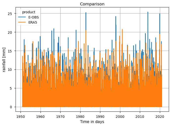
Show code cell source
# Plot a comparison between the years with maximum and minimum annual precipitation
da_timeseries_yearly = da_timeseries.sel(product="E-OBS").groupby("time.year").mean()
zooms = {
    "maximum": int(da_timeseries_yearly.idxmax("year").squeeze()),
    "minimum": int(da_timeseries_yearly.idxmin("year").squeeze()),
}
for label, year in zooms.items():
    da = da_timeseries.sel(time=str(year))
    da.plot(hue="product")
    plt.grid()
    plt.title(f"The year with the {label} is {year}")
    plt.show()
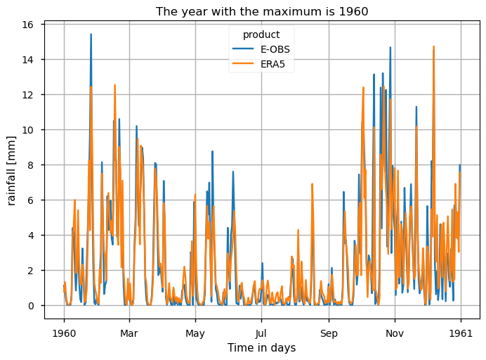
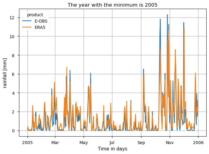
These time series plots show that both data products have very similar temporal variability and ranges in the RR values, with very few cases of RR > 20mm. Furthermore, the same level of agreement is found when the annual maximum and minimum RR values are analysed: 1960 is shown to have several days surpassing 12mm of rain, whereas in 2005 there where only two days in which these values were reached (in EOBS). ERA5 shows great agreement, with slightly lower maximum values and higher minimums.
2. Plot the climatology and the probability density function (PDF) for alternative 30-year periods#
2.1. Calculation of the Climatological Mean#
With the subsets per period already created, now it is time to calculate the climatological mean over each Time of Interest (ToI). Here, the calculation of the annual mean RR map for each day of the year (DOY) is done, while considering a 15-days Simple Moving Average (SMA), in order to smooth the inter-days varibility.
To complement the statistics and the maps of the annual mean RR over the Iberian Peninsula, it is also useful to consider the full distribution of the values of this variable, which is a function of space and time. The PDF is useful to this effect, as is shows how frequent certain values are in a given period. To this effect, we will use the helper functions defined earlier to calculate the climatology and the probability density function. In the following plot, we compare the PDF across the five climatology periods to emphasise how these frequencies have been changing.
Show code cell source
# Plot the PDF and climatology maps of RR
maps_kwargs = {"col": "period", "cmap": "jet", "robust": True}
pdf_kwargs = {"colors": colors, "hue": "period", "figsize": [15, 5]}
for da in ds_periods.data_vars.values():
    plot.projected_map(da.mean("dayofyear", keep_attrs=True), **maps_kwargs)
    plt.show()

    plot_pdf(da, **pdf_kwargs)
    plt.show()
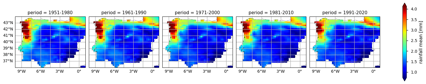
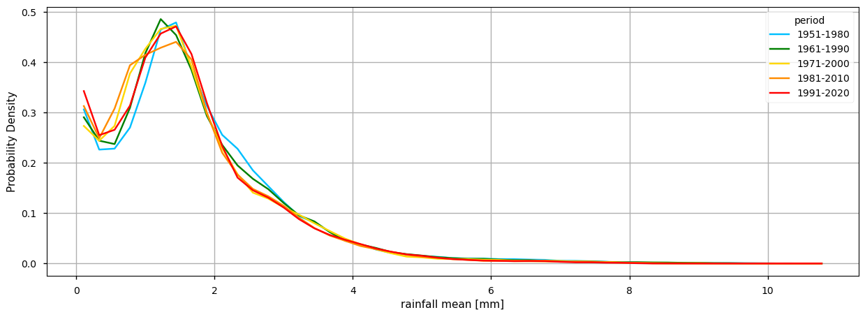
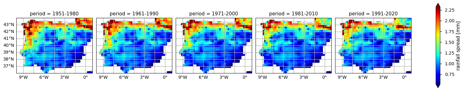
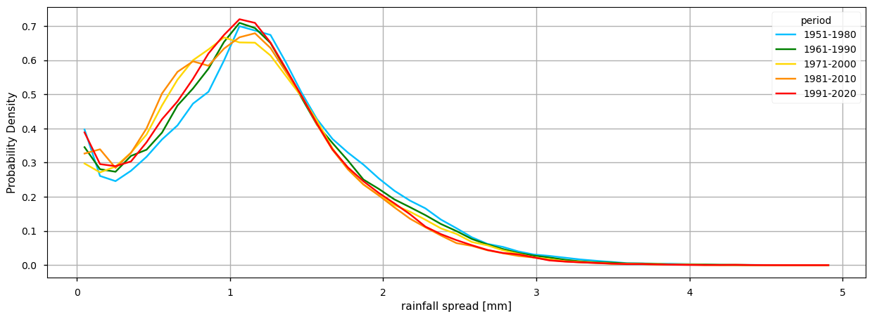
The RR climatology maps already disclose some spatial patterns of the annual statistics summarised before: for instance, the decrease of RR is more pronounced in north-western and south-eastern coastal parts of the AoI, compared to the inland region. Nevertheless, as shown in the rainfall spread maps,the northernmost part of the AoI is characterised by a larger range - this suggests that there is a lower confidence in the gridded values over this region, possibly attributable to lower density of stations or increased regional RR variability.
In addition, the PDF plots show that a gradual shift in the distribution of precipitation can be observed over time. Particularly from the earlier time period (1951-1980) represented in light blue, to the more recent periods (1991-2020) in red, there is a slight reduction of cases where average RR surpassed 2.0mm. From the rainfall spread PDF plot, it is also shown that the spread range is becoming more concentrated around certain values (below 1.5mm). This agrees with the consistent increase of in-situ data available, along time.
3. Calculate and plot seasonal PDFs and the climatological season maps#
To take the analysis further, it is also useful to proceed with the calculation of seasonal climatologies. In this case the ToI will consider all the seasons of the year, i.e., Winter (Decembre, January, and February - DJF), Spring (March, April, May - MAM), Summer (June, July, and August - JJA) and Autumn (September, October, November - SON). In both cases, we will plot their PDF and maps for all the five periods.
Show code cell source
for da in ds_periods.data_vars.values():
    plot.projected_map(
        da.groupby("season").mean(keep_attrs=True),
        row="season",
        **maps_kwargs,
    )
    plt.show()

    plot_pdf(da, col="season", **pdf_kwargs)
    plt.show()
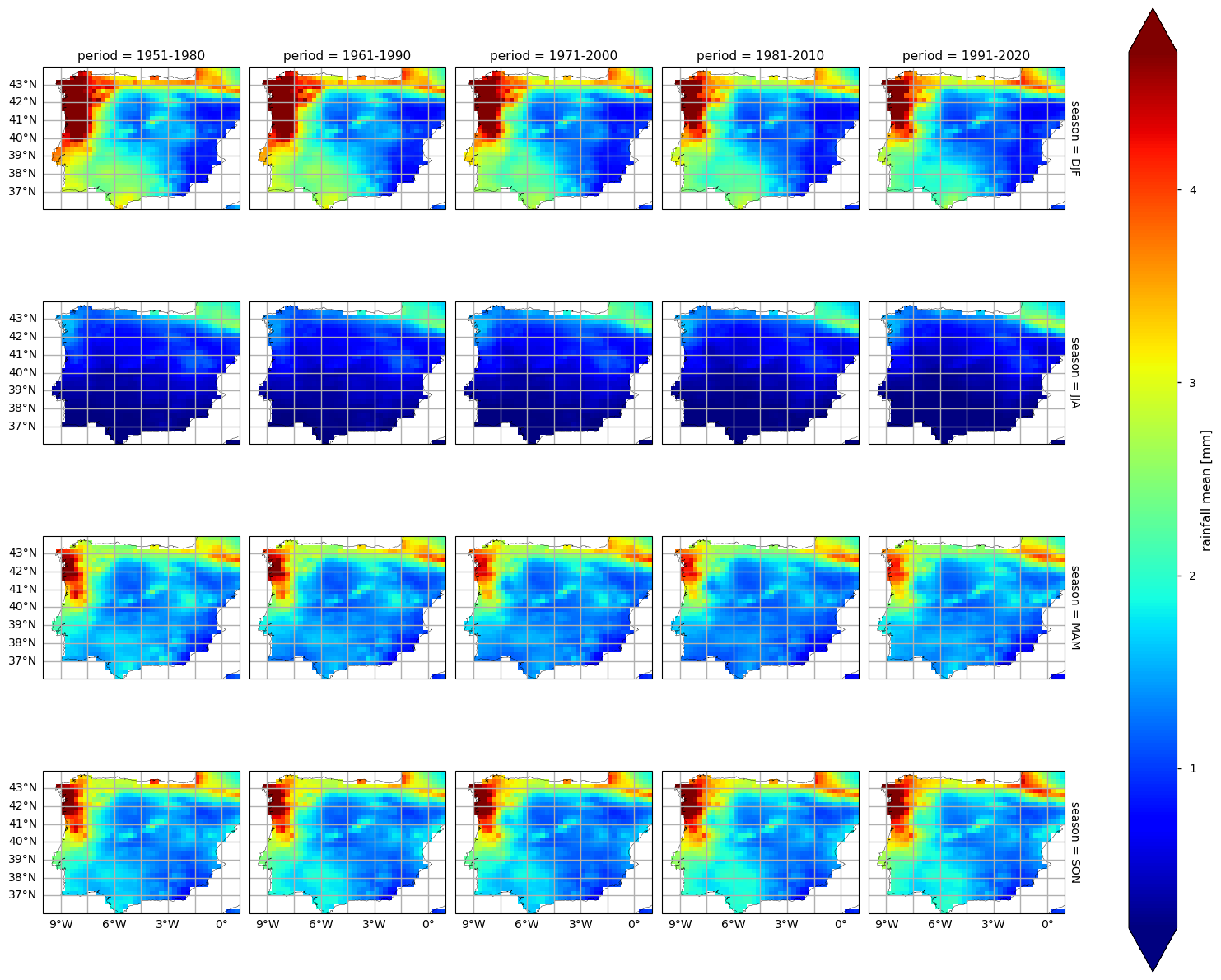
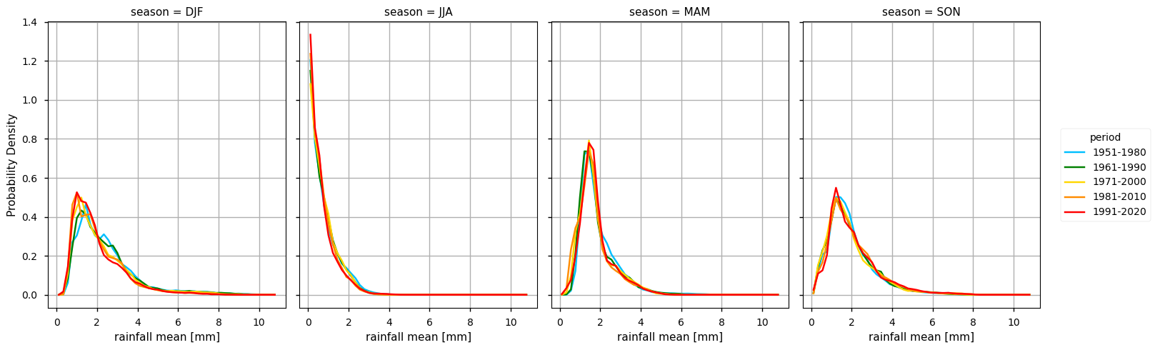
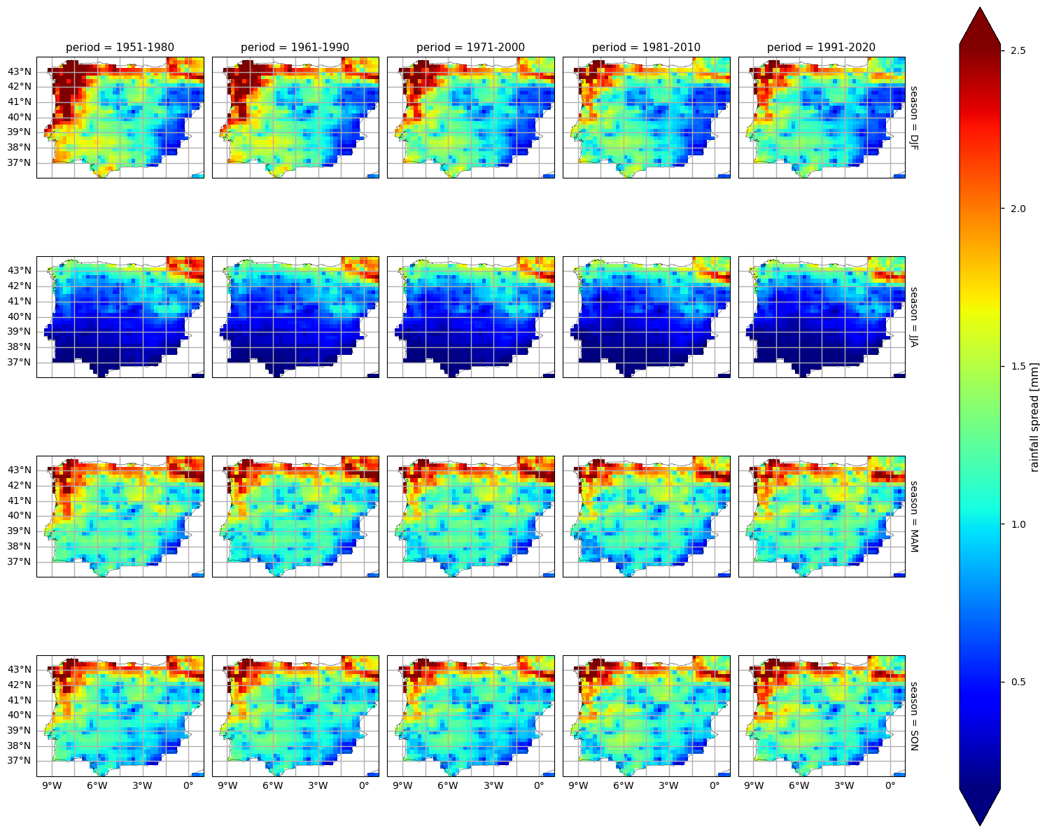
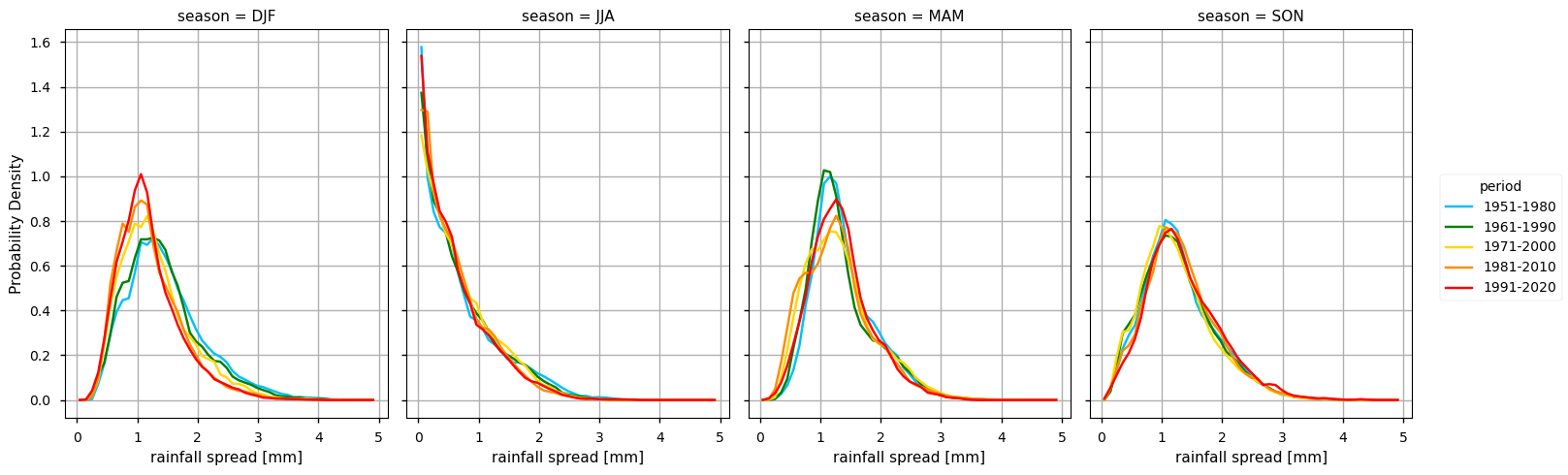
In the above plots, we can see a dissimilar spatial pattern between seasonal changes: in the Winter, the higher RR changes are clustered along the Atlantic littoral zones, namely along the Portuguese western and the Spanish northern coasts, in which pixel values above 2.5mm are becoming rarer; by contrast, in the dry Summer season, the areas with an average lack of rainfall are expanding further inland in Spain. During the transition seasons, we can see here also contrasts: while the Spring shows a decrease in overall precipitation, in the Autumn, the reduction is more pronounced in the North-western part of AoI, whereas there is a slight increase in the average precipitation over the South-western region of the Iberian Peninsula (from the South of Portugal to the South of Spain).
In complement, the ensemble spread maps illustrate the confidence level and variability that these average values may represent - as with the climatology mean, also the rainfall spread has a strong seasonality component, directly proportional to the overall rainfall mean. Hence, coastal regions to the West and North of the Iberian Peninsula are characterised by a larger spread during the Winter, Autumn and Spring seasons. While the PDF results complement these findings, the shift towards lower precipitation is very slight, when comparing the most recent and earlier periods. The only exception is the Autumn season in which such a tendency is absent.
4. Calculate the annual count of days#
To take the analysis one step further, we will calculate the the amount of days when RR≥10mm. Also called as the ‘Number of very heavy rain days’, this R10mm index is defined by WMO Expert Team on Climate Change Detection Indices, ETCCDI. We will proceed with the intercomparions of the results between both the E-OBS and ERA5 data products.
Show code cell source
# Calculate and plot the annual time series of R10mm days for E-OBS and ERA5, along with their linear trend
df = (da_timeseries > 10).groupby("time.year").sum().to_pandas()
axes = df.T.plot.bar(figsize=[15, 10], subplots=True)
for ax, (product, df_product) in zip(axes, df.groupby("product")):
    years = df_product.columns
    x_values = years - years[0]
    mk_result = mk.original_test(df_product.squeeze().values)
    slope, intercept, r_value, p_value, std_err = scipy.stats.linregress(
        x_values,
        df_product.squeeze(),
    )
    ax.plot(x_values, intercept + slope * (x_values), "k--", label="Sen's Slope")

    ax.set_ylim(top=18)

    text = "\n".join(
        [
            f"Slope: {slope:.4f} days/year",
            f"P-value: {p_value:.4f}",
            f"Tau: {mk_result.Tau:.4f}",
            f"Intercept: {intercept:.4f} days",
        ]
    )
    ax.text(1.01, 1, text, transform=ax.transAxes, fontsize=10, ha="left", va="top")
    ax.legend()
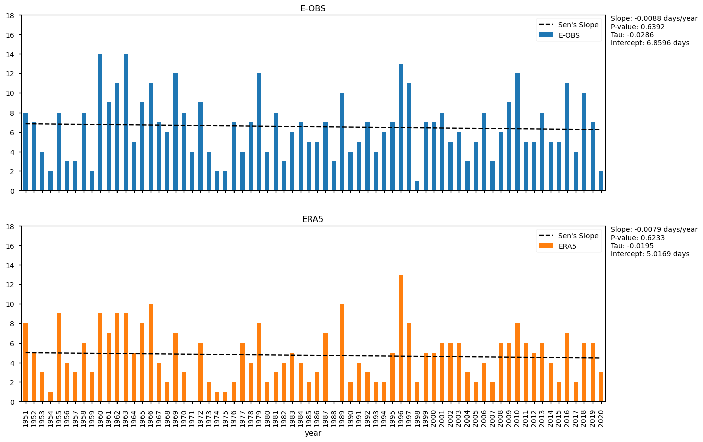
As shown in these plots, neither dataset reveals any statistically significant trend in the number of days with rainfall exceeding 10.0 mm, despite the slight RR reduction observed in the climatologies and statistics. Interestingly, both datasets have similar intercepts, slightly negative slopes, and notable inter-annual variability. Furthermore, ERA5 has slightly fewer years in which heavy precipitation occured in 6 or more days (28, compared to 34 in E-OBS), and a lower overall maximum of the two time series (12.0 mm in ERA5, compared to 14.0 mm in EOBS). Despite non-significant results, the last two decades are indeed characterised by fewer heavy precipitation days, compared to the earlier periods.
Discussion#
The analysis shows a strong overall agreement between the E-OBS and ERA5 datasets which reinforces their fitness to disclose spatio-temporal precipitation patterns, including significative precipitation events over the Iberian Peninsula, across the period of study. Over the recent decades, the data suggests a shift in precipitation patterns towards reduced rainfall, especially during the Winter and Spring, and a decrease in the frequency of extreme precipitation days. Nevertheless, inter-annual variability remains consistently high, and there is no statistically significant trend in the number of heavy precipitation days (RR ≥ 10.0 mm), between 1950 and 2020, in both datasets. Although slight downward trends are visible, they are not strong enough to be conclusive. Some minor discrepancies arise when comparing the amount of such extreme precipitation days, with ERA5 showcasing lower maximum values.
These findings show how the precipitation statistics over the Iberian Peninsula are, in fact, consistent and adequatly disclose the full temporal and spatial variability of changes in the local and regional climate. While the ensemble spread shows inhomogeneous spatial patterns that may arise from the irregular density of in-situ stations available, across the region, as well as from the variability of the precipitation over this region, the agreement with ERA5 reinforces the confidence in using the E-OBS dataset, especially when studying rainfall extremes, and further detail is required.
Nevertheless, inhomogeneities accross the region indicate that E-OBS accuracy may be location-dependent. As described in this dataset’s documentation, the usage of this dataset should be done with caution, especially when interpreting trends and extremes, considering the potential limitations in accuracy and completeness in regions where observational data may be scarcer. Furthermore, potential biases should be considered from the interpolation techniques employed, and consider the spatial variability of the variables when interpreting results. As an indicator of the confidence intervals associated with individual grid cells, the ensemble spread may provide insights into the reliability of data in specific locations, aiding in the assessment of uncertainties. In all cases, the intercomparison with reference in-situ data is advised.
5. Main takeaways#
The comparison of precipitation trends between E-OBS and ERA5 reveals several important insights. Both datasets are largely consistent in capturing overall precipitation patterns, particularly in terms of the frequency and occurrence of daily precipitation events. ERA5 and E-OBS demonstrate strong alignment in their time series, but there are some minor discrepancies in the detection of heavy rainfall days. This slight discrepancy suggests an intercomparison between E-OBS and reference stations is advised, when using this dataset for detecting rainfall extremes, particularly in data-sparse regions.
The statistically significant trends in the number of Extreme Wind Days across both datasets further supports the notion that there is no clear trend in extreme rainfall events over the observed period (1950–2020), in this region, despite an overall slight reduction in terms of climatological mean values, especially during the Winter and Spring.
When focusing on extreme events, EOBS shows the highest maximum magnitudes, which aligns with the findings from the literature, such as [5] and [7], who emphasized EOBS improved detection of extreme precipitation compared to ERA5, in areas with dense input data. However, the authors refer that this superiority is dependent on station density. Therefore, while the dataset offers consistent estimates for general precipitation trends, researchers studying extreme events should consider the ensemble spread as an indicator of confidence in extreme rainfall detection.
In conclusion, while E-OBS remains a robust dataset for historical analysis, particularly in areas with dense observational networks, it is advised to use in-situ stations data to provide complementary insights, especially in regions with sparse data coverage and for analyses focused on extreme precipitation events. The choice of dataset should thus be informed by the specific research focus.
ℹ️ If you want to know more#
Key resources#
Some key resources and further reading were linked throughout this assessment.
The CDS catalogue entry for the data used were:
E-OBS daily gridded meteorological data for Europe from 1950 to present derived from in-situ observations: https://cds.climate.copernicus.eu/datasets/insitu-gridded-observations-europe?tab=overview
ERA5 hourly data on pressure levels from 1940 to present: https://cds.climate.copernicus.eu/datasets/reanalysis-era5-pressure-levels?tab=overview
Code libraries used:
C3S EQC custom functions,
c3s_eqc_automatic_quality_control, prepared by B-Open
References#
[1] Copernicus Climate Change Service. 2024. European State of the Climate 2023.
[2] Climpact. 2024.
[3] World Meteorological Organization (WMO) Guidelines on the Calculation of Climate Normals:
[4] Cornes, R., G. van der Schrier, E.J.M. van den Besselaar, and P.D. Jones. 2018: An Ensemble Version of the E-OBS Temperature and Precipitation Datasets, J. Geophys. Res. (Atmospheres), 123.
[5] Bandhauer, Moritz, Francesco Isotta, Mónika Lakatos, Cristian Lussana, Line Båserud, Beatrix Izsák, Olivér Szentes, Ole Einar Tveito, and Christoph Frei. 2022. “Evaluation of Daily Precipitation Analyses in E-OBS (V19.0e) and ERA5 by Comparison to Regional High-Resolution Datasets in European Regions.” International Journal of Climatology 42 (2): 727–47.
[6] Hofstra, Nynke, Malcolm Haylock, Mark New, and Phil D. Jones. 2009. “Testing E-OBS European High-Resolution Gridded Data Set of Daily Precipitation and Surface Temperature.” Journal of Geophysical Research Atmospheres.
[7] Rivoire, Pauline, Olivia Martius, and Philippe Naveau. 2021. “A Comparison of Moderate and Extreme ERA-5 Daily Precipitation With Two Observational Data Sets.” Earth and Space Science 8 (4): e2020EA001633.