Assessment of the resolution capability of SLSTR AOD (1°) to identify pollution hotspots (Jan 2018–Jun 2023).

1.2.1. Assessment of the resolution capability of SLSTR AOD (1°) to identify pollution hotspots (Jan 2018–Jun 2023).#

Production date: 30-09-2024

Produced by: University of Salerno (UNISA)- (Faezeh Karimian and Fabio Madonna)

🌍 Use case: Identification of Pollution Hotspots#

❓ Quality assessment questions#

• Can the 1° SLSTR satellite AOD product distinguish urban pollution hotspots from nearby background areas over Europe?

The satellite Aerosol Properties catalogue entry provides global Aerosol Optical Depth (AOD) and fine-mode AOD (FMAOD) from 1995 to the present. AOD is often used as an indicator of particulate aerosol loading, but it represents the full atmospheric column rather than near-surface concentrations. Therefore, it may not directly capture changes in local surface air pollution, especially when aerosols are transported, vertically distributed above the boundary layer, or affected by dilution and dispersion processes [1].

In addition, several satellite aerosol products have horizontal resolutions that are coarser than the spatial scale required to resolve local differences caused by urban emission sources. Europe, where most citizens are exposed to air pollution levels above WHO guidelines [2], provides a relevant and challenging case study for evaluating the capability of satellite-based aerosol observations to identify pollution hotspots.

In this assessment, we use the SLSTR ensemble product at 1° resolution to produce seasonal maps of AOD and FMAOD over the period January 2018–June 2023, marking major urban areas such as Milan, Brussels, London, and Athens for spatial context. These maps provide a regional overview of aerosol spatial patterns and seasonal variability. We then further analyse time series over selected urban hotspots and nearby background towns to evaluate whether persistent city–background differences can be detected.

This combined map-based and time-series approach allows us to assess both the potential and the limitations of SLSTR AOD for pollution-hotspot identification. The analysis is not intended to estimate surface PM concentrations directly, but to test whether the 1° column AOD product contains a detectable urban-scale signal relative to nearby background areas.

📢 Quality assessment statement#

These are the key outcomes of this assessment

• The seasonal maps confirm broad regional patterns in AOD and FMAOD, with higher values in summer (JJA) and spring (MAM) and lower values in winter (DJF). This seasonal cycle is consistent with enhanced photochemical activity, transport of natural aerosols, and regional meteorology.

• Pairwise comparisons between megacities and their nearby towns reveal only modest differences. For Athens, mean AOD in the city is slightly higher than in Livadeia, but for Brussels, London, and Milan the rural sites often show equal or even slightly higher values.

• These small differences highlight that, at ~1° resolution, satellite AOD tends to represent regional-scale aerosol burdens rather than sharp urban hotspots. The fractional statistics support this: for example, Athens shows the city having higher AOD than the rural site in ~68% of months, while in Brussels and London the nearby towns often exceed the city.

• For the London–Northampton comparison, Northampton is used as the inland background reference. A short gap is present in [late 2019 to early 2020], where valid monthly AOD/FMAOD values are unavailable for the Northampton AOI after filtering; these months are excluded from the paired statistics.

• Taken together, these findings emphasize the importance of scale and representativity. While satellite AOD products capture regional patterns and seasonality well, they cannot be expected to resolve contrasts between neighboring urban and rural sites at the scale of tens of kilometers.

📋 Methodology#

This assessment evaluates the capability of SLSTR-derived satellite AOD and FMAOD to capture seasonal aerosol variability and urban–background contrasts over selected European regions from January 2018 to June 2023. Data completeness is quantified using monthly valid-observation counts normalized by area. Urban–background contrasts are then tested using grid-aware neighborhoods around selected city and reference locations.

The analysis uses monthly SLSTR/Sentinel-3 AOD and FMAOD from January 2018 to June 2023 over a European domain defined by longitude −12° to 35°E and latitude 34° to 60°N. Within this domain, four paired Areas of Interest (AOIs) are selected to compare large urban areas with nearby lower-density reference locations: Athens–Livadeia in Greece, London–Northampton in the United Kingdom, Brussels–Arras in Belgium/France, and Milan–Sondrio in Italy.

The selected AOIs are based on fixed latitude/longitude coordinates. Each city is paired with a nearby town or background location within approximately 90–100 km. This design keeps each pair within a broadly similar regional aerosol environment while testing whether the 1° SLSTR product can detect persistent city–background differences in AOD and FMAOD.

The reference locations are not all purely rural sites. They were selected as nearby lower-density/background locations outside the main metropolitan areas, while remaining within the same broad regional aerosol environment. Therefore, the analysis is described as an urban–background comparison rather than a strictly urban–rural comparison. This provides a conservative test: if the reference location also contains anthropogenic emissions, the city–background contrast may be reduced.

To assess whether the 1° SLSTR AOD product can identify pollution hotspots, we define a set of verification steps before interpreting the results. Since no independent surface PM or AERONET validation dataset is used here, the verification is based on internal consistency between spatial maps, urban–background time series, and pairwise statistics.

First, the monthly time series of AOD550 and FM_AOD550 are compared between each urban hotspot and its nearby background reference area. If the product can detect an urban aerosol enhancement, the city should show higher AOD and/or FM_AOD than the background area for a substantial fraction of valid months. To reduce the influence of individual monthly peaks, 3-month rolling means are also shown as a visual guide, while the statistics are calculated from the original monthly values.

Second, pairwise city–background differences are calculated as:

ΔAOD = AOD_city − AOD_background

and similarly for FM_AOD550. For each pair, the mean difference, the 95% confidence interval, and the fraction of valid months in which the city value is higher than the background value are used to evaluate whether the urban signal is persistent. A robust signal would require a positive mean difference, a confidence interval that does not strongly overlap zero, and a city-higher fraction greater than 0.5.

Third, seasonal climatological maps of AOD550 and FM_AOD550 are used to check whether the selected city and background locations are embedded in broader regional aerosol patterns. This step is important because AOD is a column-integrated quantity and may be influenced by transported aerosols, sea salt, dust, humidity effects, and regional pollution plumes. Therefore, a city–background contrast is interpreted only in the context of the surrounding seasonal spatial pattern.

Finally, focused seasonal maps are produced for each city–background pair. These maps check whether the local pairwise contrast seen in the time series is spatially consistent with the surrounding 1° grid cells. If both the city and background locations lie within the same broad aerosol plume, weak city–background differences are expected and should not be interpreted only as a failure of spatial resolution.

The methodology adopted for the analysis is split into the following steps:

Choose the data to use and set up the code

Import all required libraries

Data Retrieval and Preparation

Retrieve and prepare AOD/FMAOD data
Prepare the dataframe
Define required functions

Plot, calculation and describe the results

Pairwise monthly differences (city − background)
Seasonal mean contrasts per urban–background pair
Urban–background AOD and FM-AOD time-series plots
Seasonal AOD and FM-AOD maps with urban/background markers
Focused seasonal map plots of AOD550 and FM_AOD550 for selected urban–background pairs

Take-Home Messages

Main takeaways and limitations

Selection of urban hotspots and background reference areas#

The analysis focuses on four European urban hotspots and their nearby background reference areas: Athens–Livadeia, London–Northampton, Brussels–Arras, and Milan–Sondrio. The selected locations are within the European domain defined above and are separated by approximately 90–100 km.

The background locations are not intended to represent perfectly clean rural sites. Instead, they are selected as lower-density reference areas outside the main metropolitan regions, while remaining within the same broad regional aerosol environment as the corresponding city. This design allows a conservative test of whether the 1° SLSTR AOD product can detect persistent urban–background differences in AOD550 and FM_AOD550.

Rather than comparing urban areas with purely rural backgrounds, this assessment intentionally focuses on the contrast between major metropolitan areas (large cities) and nearby smaller urban centers (small cities). A conventional city-rural comparison cannot reveal the sensitivity of satellite instrument in capturing different kind of pollution hotspots from the Aerosol Optical Depth (AOD) products. By comparing distinct urban nodes of varying sizes (large vs. small cities) within the same regional background, we provide a more robust and sensitive evaluation of the satellite’s capability to detect localized anthropogenic emission gradients.

📈 Analysis and results#

Choose the data to use and set up the code#

Import all required libraries#

In this section, we import all the relevant packages needed for running the notebook.

Data Retrieval and Preparation#

Below are robust, grid-aware functions and the city/rural time-series computation.

Download AOD data#

Found 66 .nc files
./aod_data/201801-C3S-L3_AEROSOL-AER_PRODUCTS-SLSTR-SENTINEL3A-ensemble-MONTHLY-v2.3.nc
./aod_data/201802-C3S-L3_AEROSOL-AER_PRODUCTS-SLSTR-SENTINEL3A-ensemble-MONTHLY-v2.3.nc
./aod_data/201803-C3S-L3_AEROSOL-AER_PRODUCTS-SLSTR-SENTINEL3A-ensemble-MONTHLY-v2.3.nc
./aod_data/201804-C3S-L3_AEROSOL-AER_PRODUCTS-SLSTR-SENTINEL3A-ensemble-MONTHLY-v2.3.nc
./aod_data/201805-C3S-L3_AEROSOL-AER_PRODUCTS-SLSTR-SENTINEL3A-ensemble-MONTHLY-v2.3.nc
              time  latitude  longitude    AOD550  FM_AOD550  \
0       2018-01-01     -89.5     -179.5       NaN        NaN   
43192   2018-01-01      29.5      172.5  0.123682   0.049830   
43193   2018-01-01      29.5      173.5  0.116795   0.043411   
43194   2018-01-01      29.5      174.5  0.188018   0.079148   
43195   2018-01-01      29.5      175.5  0.058454   0.015076   
...            ...       ...        ...       ...        ...   
4233604 2023-06-01     -29.5     -175.5  0.076325   0.047782   
4233605 2023-06-01     -29.5     -174.5  0.069183   0.040526   
4233606 2023-06-01     -29.5     -173.5  0.071204   0.041869   
4233593 2023-06-01     -30.5      173.5  0.093562   0.054036   
4276799 2023-06-01      89.5      179.5       NaN        NaN   

         AOD550_UNCERTAINTY_ENSEMBLE  NMEAS  
0                                NaN    0.0  
43192                       0.004982    6.0  
43193                       0.004510    4.0  
43194                       0.005259    3.0  
43195                       0.000400    1.0  
...                              ...    ...  
4233604                     0.017169   11.0  
4233605                     0.014429   12.0  
4233606                     0.013793   11.0  
4233593                     0.015986    6.0  
4276799                          NaN    0.0  

[4276800 rows x 7 columns]

Prepare the dataframe#

In this step, the monthly SLSTR gridded dataset is prepared for seasonal and regional analysis. The analysis is restricted to the European domain defined above and to the period 2018–2023. Time information is then expanded into year, month, season, and season-year columns.

The season_year column is introduced to handle winter consistently: December is assigned to the following year, so that DJF represents one continuous winter season. After these time labels are added, seasonal mean AOD550 and FM_AOD550 values are computed for each grid cell.

Although the original data are gridded, the dataframe format is used here to simplify the later city–background pairwise statistics. Spatial aggregation for the city–background comparison is performed using fixed grid-aware neighbourhoods around each AOI. The use of dataframes is therefore limited to the tabular comparison step, where monthly city and background values are joined and differenced.

Define required functions#

The following functions are used to make the analysis reproducible and easier to interpret.

First, month_to_season assigns each month to a meteorological season: DJF, MAM, JJA, or SON. The function seasonal_means then calculates the seasonal mean AOD550 and FM_AOD550 for each grid cell, preserving the latitude and longitude structure needed for mapping.

The plotting functions convert the seasonal dataframe back into a regular latitude–longitude grid for visualization. grid_for_plot creates the grid edges required by pcolormesh, while plot_seasonal_maps displays seasonal climatological maps and marks the selected urban and background AOIs.

For the city–background analysis, monthly values are extracted from a grid-aware neighbourhood around each AOI. The neighbourhood size is defined by HALFWIN = 0.5, corresponding approximately to the native 1° SLSTR grid cell around the selected latitude/longitude point. For each city–background pair, the monthly difference is computed as:

ΔAOD = AOD_city − AOD_background

and similarly for FM_AOD550. The metric frac_city_gt is the percentage of valid months in which the city value is higher than the background value. For example, frac_city_gt = 60% means that the city had higher AOD than the background in 60% of the valid monthly comparisons.

The 3-month rolling mean shown in the time-series plots is used only for visualization, to reduce month-to-month noise and highlight persistent behaviour. The pairwise statistics are calculated from the original monthly values, not from the rolling curves.

Show code cell source

Hide code cell source

def month_to_season(m):
    # DJF, MAM, JJA, SON
    if m in (12, 1, 2):
        return "DJF"
    elif m in (3, 4, 5):
        return "MAM"
    elif m in (6, 7, 8):
        return "JJA"
    else:
        return "SON"


def seasonal_means(df, value_cols=("AOD550", "FM_AOD550")):
    # drop entirely NaN rows for both vars
    keep = df.copy()
    # group per (season_year, season, lat, lon)
    grp = keep.groupby(["season_year","season","latitude","longitude"], as_index=False)[list(value_cols)].mean()
    return grp


def grid_for_plot(df_season, var):
    
    grid = df_season.pivot_table(index="latitude", columns="longitude", values=var, aggfunc="mean")
    lats = grid.index.values
    lons = grid.columns.values

    dlat = np.median(np.diff(lats)) if len(lats) > 1 else 1.0
    dlon = np.median(np.diff(lons)) if len(lons) > 1 else 1.0
    lat_edges = np.concatenate(([lats[0]-dlat/2], (lats[:-1]+lats[1:])/2, [lats[-1]+dlat/2]))
    lon_edges = np.concatenate(([lons[0]-dlon/2], (lons[:-1]+lons[1:])/2, [lons[-1]+dlon/2]))
    return lon_edges, lat_edges, grid.values

import matplotlib.gridspec as gridspec

def plot_seasonal_maps(seasonal_df, var, season_year=None, cmap="viridis",
                       vmin=None, vmax=None, extent=EUROPE_EXTENT, title_suffix=""):

    df = seasonal_df.copy()
    if season_year is not None:
        df = df[df["season_year"] == season_year]
    else:
        df = df.groupby(["season","latitude","longitude"], as_index=False)[var].mean()

    seasons = ["DJF","MAM","JJA","SON"]
    proj = ccrs.PlateCarree()


    fig = plt.figure(figsize=(15, 9))
    gs = gridspec.GridSpec(2, 3, width_ratios=[1,1,0.05])  

    axes = []
    for i in range(2):
        for j in range(2):
            ax = fig.add_subplot(gs[i, j], projection=proj)
            axes.append(ax)

    for ax, s in zip(axes, seasons):
        sub = df[df["season"] == s]
        if sub.empty:
            ax.set_title(f"{s} (no data)")
            ax.coastlines(); ax.add_feature(cfeature.BORDERS, linewidth=0.4)
            ax.set_extent(extent, crs=proj); continue

        lon_edges, lat_edges, Z = grid_for_plot(sub, var)

        mesh = ax.pcolormesh(lon_edges, lat_edges, Z, transform=proj,
                             cmap=cmap, shading="auto", vmin=vmin, vmax=vmax)
        ax.coastlines()
        ax.add_feature(cfeature.BORDERS, linewidth=0.4)
        ax.add_feature(cfeature.LAND, facecolor="none", edgecolor="black", linewidth=0.2)
        ax.set_extent(extent, crs=proj)
        ax.set_title(f"{s}")

        for name, info in AOIS.items():
            if (extent[0] <= info["lon"] <= extent[1]) and (extent[2] <= info["lat"] <= extent[3]):
                mk = "s" if info["kind"] == "city" else "o"
                ax.plot(info["lon"], info["lat"], mk, transform=proj, ms=5, mec="k", mfc="none")
                ax.text(info["lon"]+0.3, info["lat"]+0.3, name.split(" (")[0],
                        transform=proj, fontsize=8)

    cax = fig.add_subplot(gs[:, 2])
    cbar = fig.colorbar(mesh, cax=cax)
    cbar.set_label(var)

    title_year = f"{season_year}" if season_year is not None else "Climatology"
    fig.suptitle(f"SLSTR seasonal mean {var} — {title_year} {title_suffix}", y=0.95, fontsize=14)

    plt.tight_layout(rect=[0,0,0.93,0.95])
    return fig






def global_color_limits(seasonal_df, var, lo=5, hi=95):
    vals = seasonal_df[var].to_numpy()
    return (np.nanpercentile(vals, lo), np.nanpercentile(vals, hi))

def subset_seasonal_box(seasonal_df, extent):
    w,e,s,n = extent
    return seasonal_df[
        (seasonal_df["longitude"]>=w) & (seasonal_df["longitude"]<=e) &
        (seasonal_df["latitude"] >=s) & (seasonal_df["latitude"] <=n)
    ]

def grid_for_plot(df_season, var):
    grid = df_season.pivot_table(index="latitude", columns="longitude", values=var, aggfunc="mean")
    lats = grid.index.values
    lons = grid.columns.values
    dlat = np.median(np.diff(lats)) if len(lats)>1 else 1.0
    dlon = np.median(np.diff(lons)) if len(lons)>1 else 1.0
    lat_edges = np.concatenate(([lats[0]-dlat/2], (lats[:-1]+lats[1:])/2, [lats[-1]+dlat/2]))
    lon_edges = np.concatenate(([lons[0]-dlon/2], (lons[:-1]+lons[1:])/2, [lons[-1]+dlon/2]))
    return lon_edges, lat_edges, grid.values


if 'df_eu' not in globals():
  
    EUROPE_EXTENT = (-12, 35, 34, 60)
    df_eu = final_df[
        (final_df['longitude']>=EUROPE_EXTENT[0]) & (final_df['longitude']<=EUROPE_EXTENT[1]) &
        (final_df['latitude'] >=EUROPE_EXTENT[2]) & (final_df['latitude'] <=EUROPE_EXTENT[3])
    ].copy()
    df_eu = df_eu[(df_eu['time'].dt.year>=2018) & (df_eu['time'].dt.year<=2023)]
    df_eu = df_eu.assign(month=df_eu['time'].dt.month,
                         year=df_eu['time'].dt.year)
    def m2s(m):
        return "DJF" if m in (12,1,2) else ("MAM" if m in (3,4,5) else ("JJA" if m in (6,7,8) else "SON"))
    df_eu['season'] = df_eu['month'].apply(m2s)
    df_eu['season_year'] = df_eu['year']
    df_eu.loc[df_eu['month']==12,'season_year'] = df_eu['year']+1

seasonal = (df_eu
            .groupby(["season_year","season","latitude","longitude"], as_index=False)
            [["AOD550","FM_AOD550"]].mean())

aod_vmin, aod_vmax = global_color_limits(seasonal, "AOD550", 5, 95)
fm_vmin,  fm_vmax  = global_color_limits(seasonal, "FM_AOD550", 5, 95)

import numpy.ma as ma

def plot_pair_focus(
    pair,
    var="AOD550",
    cmap="YlOrRd",
    vmin=None,
    vmax=None,
    pad_deg=0.25,  
    title_suffix="Climatology (2018–2023)"
):
    city, town = pair
    c = AOIS[city]; r = AOIS[town]

 
    clim = seasonal.groupby(["season","latitude","longitude"], as_index=False)[var].mean()

 
    w = min(c["lon"], r["lon"]) - pad_deg
    e = max(c["lon"], r["lon"]) + pad_deg
    s = min(c["lat"], r["lat"]) - pad_deg
    n = max(c["lat"], r["lat"]) + pad_deg
    box = subset_seasonal_box(clim, (w, e, s, n))


    if not box.empty:
        w = float(box["longitude"].min()) - 0.25
        e = float(box["longitude"].max()) + 0.25
        s = float(box["latitude"].min()) - 0.25
        n = float(box["latitude"].max()) + 0.25
    extent = (w, e, s, n)


    fig = plt.figure(figsize=(10, 6))
    gs = gridspec.GridSpec(2, 3, width_ratios=[1,1,0.05], wspace=0.1, hspace=0.15)
    axes = [
        fig.add_subplot(gs[0,0], projection=ccrs.PlateCarree()),
        fig.add_subplot(gs[0,1], projection=ccrs.PlateCarree()),
        fig.add_subplot(gs[1,0], projection=ccrs.PlateCarree()),
        fig.add_subplot(gs[1,1], projection=ccrs.PlateCarree()),
    ]
    cax = fig.add_subplot(gs[:,2])


    base_cmap = plt.get_cmap(cmap).copy()
    low_col = base_cmap(0.0)
    base_cmap.set_bad(low_col)
    base_cmap.set_under(low_col)

    last_mesh = None
    for ax, season in zip(axes, ["DJF","MAM","JJA","SON"]):
        sub = box[box["season"]==season]
        ax.set_title(season)
        ax.set_extent(extent)
        ax.coastlines()
        ax.add_feature(cfeature.BORDERS, linewidth=0.4)
        ax.set_facecolor(low_col)

        if not sub.empty:
            loE, laE, Z = grid_for_plot(sub, var)
            Z_masked = ma.masked_invalid(Z)
            last_mesh = ax.pcolormesh(loE, laE, Z_masked, cmap=base_cmap,
                                      transform=ccrs.PlateCarree(),
                                      shading="auto", vmin=vmin, vmax=vmax)

 
        ax.plot(c["lon"], c["lat"], "s", ms=6, mec="k", mfc="white", transform=ccrs.PlateCarree())
        ax.plot(r["lon"], r["lat"], "o", ms=6, mec="k", mfc="white", transform=ccrs.PlateCarree())

    if last_mesh:
        cb = fig.colorbar(last_mesh, cax=cax)
        cb.set_label(var)

    fig.suptitle(f"{var} — {city} vs {town} — {title_suffix}", y=0.97)
    plt.tight_layout(rect=[0,0,0.95,0.95])
    import matplotlib.lines as mlines


    city_marker = mlines.Line2D([], [], color="black", marker="s", linestyle="None",
                            markersize=6, label="City (megacity)")
    rural_marker = mlines.Line2D([], [], color="black", marker="o", linestyle="None",
                             markersize=6, label="Rural (nearby town)")

    fig.legend(handles=[city_marker, rural_marker], loc="lower center", ncol=2, frameon=False)

    return fig, extent



def ensure_monthly(df):
    df = df.copy()
    df["time"] = pd.to_datetime(df["time"]).dt.to_period("M").dt.to_timestamp()
    return df

final_df = ensure_monthly(final_df)


def aoi_monthly_series(df, lat, lon, halfwin=0.5):
    sub = df[
        (df["latitude"].between(lat - halfwin, lat + halfwin)) &
        (df["longitude"].between(lon - halfwin, lon + halfwin))
    ]
    ser = (sub
           .groupby("time", as_index=False)[["AOD550","FM_AOD550","NMEAS"]]
           .mean()) 
    ser = ser.sort_values("time").reset_index(drop=True)
    return ser

def build_pair_df(df, city_name, town_name, halfwin=0.5):
    c = AOIS[city_name]; t = AOIS[town_name]
    city = aoi_monthly_series(df, c["lat"], c["lon"], halfwin).rename(
        columns={"AOD550":"AOD_city", "FM_AOD550":"FM_city", "NMEAS":"N_city"})
    town = aoi_monthly_series(df, t["lat"], t["lon"], halfwin).rename(
        columns={"AOD550":"AOD_town", "FM_AOD550":"FM_town", "NMEAS":"N_town"})
    merged = pd.merge(city[["time","AOD_city","FM_city"]],
                      town[["time","AOD_town","FM_town"]],
                      on="time", how="outer").sort_values("time")

    for col in ["AOD_city","AOD_town","FM_city","FM_town"]:
        merged[col+"_roll3"] = merged[col].rolling(3, center=True, min_periods=1).mean()
 
    merged["AOD_diff"] = merged["AOD_city"] - merged["AOD_town"]
    merged["FM_diff"]  = merged["FM_city"]  - merged["FM_town"]
    return merged


def plot_pair_timeseries(pair_df, city_name, town_name, year_start=2018, year_end=2023):
 
    mask = (pair_df["time"].dt.year >= year_start) & (pair_df["time"].dt.year <= year_end)
    dfp = pair_df.loc[mask].copy()

    aod_pct = np.round(100*np.nanmean(dfp["AOD_diff"] > 0), 1)
    fm_pct  = np.round(100*np.nanmean(dfp["FM_diff"]  > 0), 1)
    aod_md  = np.nanmean(dfp["AOD_diff"])
    fm_md   = np.nanmean(dfp["FM_diff"])

    fig, axes = plt.subplots(2, 1, figsize=(12, 7), sharex=True)
    ax1, ax2 = axes

    ax1.plot(dfp["time"], dfp["AOD_city"], lw=1, alpha=0.4, label=f"{city_name} (monthly)")
    ax1.plot(dfp["time"], dfp["AOD_town"], lw=1, alpha=0.4, label=f"{town_name} (monthly)")
    ax1.plot(dfp["time"], dfp["AOD_city_roll3"], lw=2.2, label=f"{city_name} (roll-3)")
    ax1.plot(dfp["time"], dfp["AOD_town_roll3"], lw=2.2, label=f"{town_name} (roll-3)")
    ax1.set_ylabel("AOD550")
    ax1.set_title("AOD550 — city vs nearby town")
    ax1.grid(alpha=0.25)
    ax1.legend(ncol=2, fontsize=9)
    ax1.text(0.01, 0.95, f"Δ = city − town | mean Δ={aod_md:.3f}, city>town={aod_pct}%",
             transform=ax1.transAxes, va="top", ha="left", fontsize=9,
             bbox=dict(boxstyle="round,pad=0.25", fc="white", ec="0.7", alpha=0.9))

    ax2.plot(dfp["time"], dfp["FM_city"], lw=1, alpha=0.4, label=f"{city_name} (monthly)")
    ax2.plot(dfp["time"], dfp["FM_town"], lw=1, alpha=0.4, label=f"{town_name} (monthly)")
    ax2.plot(dfp["time"], dfp["FM_city_roll3"], lw=2.2, label=f"{city_name} (roll-3)")
    ax2.plot(dfp["time"], dfp["FM_town_roll3"], lw=2.2, label=f"{town_name} (roll-3)")
    ax2.set_ylabel("FM_AOD550")
    ax2.set_title("Fine-mode AOD — city vs nearby town")
    ax2.grid(alpha=0.25)
    ax2.legend(ncol=2, fontsize=9)
    ax2.text(0.01, 0.95, f"Δ = city − town | mean Δ={fm_md:.3f}, city>town={fm_pct}%",
             transform=ax2.transAxes, va="top", ha="left", fontsize=9,
             bbox=dict(boxstyle="round,pad=0.25", fc="white", ec="0.7", alpha=0.9))

    fig.suptitle(f"{city_name} vs {town_name} — Monthly time series (Jan 2018–Jun 2023)", y=0.98, fontsize=13)
    ax2.set_xlabel("Time")
    fig.tight_layout(rect=[0,0,1,0.965])
    return fig   

def extract_monthly_aoi_means(df, AOIS, varlist=["AOD550","FM_AOD550"], halfwin=0.5):
    """
    Compute monthly average AOD values for each AOI (city/rural).
    """
    out = []
    for name, info in AOIS.items():
        sub = df[
            (df["longitude"] >= info["lon"]-halfwin) & (df["longitude"] <= info["lon"]+halfwin) &
            (df["latitude"]  >= info["lat"]-halfwin) & (df["latitude"]  <= info["lat"]+halfwin)
        ].copy()
        if sub.empty:
            continue
        tmp = sub.groupby([df["time"].dt.year, df["time"].dt.month])[varlist].mean().reset_index()
        tmp.columns = ["year","month"] + varlist
        tmp["AOI"] = name
        tmp["kind"] = info["kind"]
        out.append(tmp)
    return pd.concat(out, ignore_index=True)

def extract_monthly_aoi_means(df, AOIS, varlist=("AOD550","FM_AOD550"), halfwin=0.5):
    """
    Returns a DataFrame with columns:
    ['AOI','kind','year','month','AOD550','FM_AOD550']
    """
    df = df.copy()
 
    df["time"] = pd.to_datetime(df["time"]).dt.to_period("M").dt.to_timestamp()

    out = []
    for name, info in AOIS.items():
        sub = df[
            (df["longitude"].between(info["lon"]-halfwin, info["lon"]+halfwin)) &
            (df["latitude"].between(info["lat"]-halfwin, info["lat"]+halfwin))
        ].copy()
        if sub.empty:
            continue

 
        sub["year"] = sub["time"].dt.year
        sub["month"] = sub["time"].dt.month

        tmp = (sub.groupby(["year","month"], as_index=False)[list(varlist)]
                  .mean())
        tmp["AOI"] = name
        tmp["kind"] = info["kind"]
        out.append(tmp)

    return pd.concat(out, ignore_index=True) if out else pd.DataFrame(
        columns=["AOI","kind","year","month",*varlist]
    )

monthly_df = extract_monthly_aoi_means(final_df, AOIS, varlist=("AOD550","FM_AOD550"), halfwin=0.5)


def monthly_pairwise_diff(monthly_df, pairs):
    diffs = []
    for city, town in pairs:
        c = monthly_df[monthly_df["AOI"] == city].copy()
        r = monthly_df[monthly_df["AOI"] == town].copy()
        merged = pd.merge(c, r, on=["year","month"], suffixes=("_city","_rural"))
        merged["AOD550_diff"]    = merged["AOD550_city"]    - merged["AOD550_rural"]
        merged["FM_AOD550_diff"] = merged["FM_AOD550_city"] - merged["FM_AOD550_rural"]
        merged["pair"] = f"{city} − {town}"
        diffs.append(merged[["year","month","pair","AOD550_diff","FM_AOD550_diff"]])
    return pd.concat(diffs, ignore_index=True)

pairwise_monthly = monthly_pairwise_diff(monthly_df, PAIRS)


def paired_summary(city_label, rural_label, var="AOD550"):
    c = monthly_df[monthly_df["AOI"] == city_label].copy()
    r = monthly_df[monthly_df["AOI"] == rural_label].copy()
    merged = pd.merge(c, r, on=["year","month"], suffixes=("_city","_rural"))
    diff = merged[f"{var}_city"] - merged[f"{var}_rural"]
    return {
        "pair": f"{city_label} − {rural_label}",
        "variable": var,
        "mean_diff": float(diff.mean()),
        "frac_city_gt (%)": float((diff > 0).mean()*100),
        "n_months": int(len(diff))
    }

HALFWIN = 0.5  # degrees (±0.5° = the native 1° grid cell)
YEAR_START, YEAR_END = 2018, 2023

def month_to_season(m):
    return ("DJF" if m in (12,1,2)
            else "MAM" if m in (3,4,5)
            else "JJA" if m in (6,7,8)
            else "SON")

def aoi_monthly(df, lat, lon, halfwin=0.5):
    """Monthly mean for an AOI (AOD550 & FM_AOD550) from the 1° grid cell around (lat,lon)."""
    sub = df[
        df["latitude"].between(lat-halfwin, lat+halfwin) &
        df["longitude"].between(lon-halfwin, lon+halfwin)
    ].copy()
    if sub.empty:
        return pd.DataFrame(columns=["time","AOD550","FM_AOD550","season"])

    sub["time"] = pd.to_datetime(sub["time"]).dt.to_period("M").dt.to_timestamp()
    sub = sub[(sub["time"].dt.year >= YEAR_START) & (sub["time"].dt.year <= YEAR_END)]

    out = (sub.groupby("time", as_index=False)[["AOD550","FM_AOD550"]].mean()
              .sort_values("time"))
    out["season"] = out["time"].dt.month.map(month_to_season)
    return out

ts_by_place = {}
for name, info in AOIS.items():
    ts_by_place[name] = aoi_monthly(final_df, info["lat"], info["lon"], halfwin=HALFWIN)

print("\nSeasonal means (climatological) per pair:")

def print_pair_seasonals(city_label, background_label, var):
    c = ts_by_place[city_label]
    r = ts_by_place[background_label]

    c_seas = c.groupby("season", as_index=True)[var].mean()
    r_seas = r.groupby("season", as_index=True)[var].mean()

    order = ["DJF", "MAM", "JJA", "SON"]
    c_seas = c_seas.reindex(order)
    r_seas = r_seas.reindex(order)

    out = pd.DataFrame(
        {"city": c_seas.values, "background": r_seas.values},
        index=order
    )

    print(f"\n{var} seasonal mean | {city_label} vs {background_label}")
    print(out.round(3))

Seasonal means (climatological) per pair:

Plot, calculation and describe the results#

Pairwise monthly differences (city − nearby town)#

For each urban–background pair, monthly AOD550 and FM_AOD550 values are joined by year and month. The monthly difference is then calculated as the city value minus the background value. Positive values indicate months when the urban AOI has higher column aerosol loading than the reference location.

The summary table reports:

mean_diff: the average city–background difference over all valid months;
frac_city_gt (%): the percentage of valid months for which the city value is greater than the background value;
n_months: the number of valid monthly comparisons used.

These metrics are used to assess persistence. A single high-AOD month is not enough to identify a robust hotspot signal; the city should exceed the background location in a substantial fraction of valid months.

Pairwise monthly differences (city − background):
                                                    pair  variable  mean_diff  frac_city_gt (%)  n_months
     Athens (urban hotspot) − Livadeia (background area)    AOD550      0.005            56.061        66
     Athens (urban hotspot) − Livadeia (background area) FM_AOD550      0.001            51.515        66
  London (urban hotspot) − Northampton (background town)    AOD550      0.037            65.152        66
  London (urban hotspot) − Northampton (background town) FM_AOD550      0.052            74.242        66
      Brussels (urban hotspot) − Arras (background town)    AOD550     -0.021            24.242        66
      Brussels (urban hotspot) − Arras (background town) FM_AOD550     -0.031            19.697        66
Milan (urban hotspot) − Sondrio (background valley/town)    AOD550      0.010            57.576        66
Milan (urban hotspot) − Sondrio (background valley/town) FM_AOD550      0.015            66.667        66

The results indicate that mean differences are generally small (within ±0.01–0.02), with Athens showing the most frequent positive city–rural contrast, while in Brussels, London, and Milan the rural sites often equal or exceed the city values.

Seasonal mean contrasts per urban–background pair#

For each pair, seasonal climatological means are computed from the monthly AOI time series. The table reports the mean seasonal AOD550 and FM_AOD550 for the city and the background reference location, together with the city-minus-background difference. This helps identify whether any urban enhancement is seasonally persistent or limited to specific seasons.

AOD550 seasonal mean | Athens (urban hotspot) vs Livadeia (background area)
      city  background
DJF  0.123       0.133
MAM  0.186       0.166
JJA  0.198       0.203
SON  0.155       0.141

FM_AOD550 seasonal mean | Athens (urban hotspot) vs Livadeia (background area)
      city  background
DJF  0.094       0.111
MAM  0.145       0.133
JJA  0.177       0.177
SON  0.126       0.116

AOD550 seasonal mean | London (urban hotspot) vs Northampton (background town)
      city  background
DJF  0.119       0.107
MAM  0.214       0.141
JJA  0.199       0.171
SON  0.138       0.112

FM_AOD550 seasonal mean | London (urban hotspot) vs Northampton (background town)
      city  background
DJF  0.102       0.085
MAM  0.190       0.111
JJA  0.172       0.104
SON  0.115       0.084

AOD550 seasonal mean | Brussels (urban hotspot) vs Arras (background town)
      city  background
DJF  0.149       0.146
MAM  0.152       0.183
JJA  0.197       0.222
SON  0.138       0.155

FM_AOD550 seasonal mean | Brussels (urban hotspot) vs Arras (background town)
      city  background
DJF  0.127       0.124
MAM  0.116       0.155
JJA  0.131       0.178
SON  0.113       0.135

AOD550 seasonal mean | Milan (urban hotspot) vs Sondrio (background valley/town)
      city  background
DJF  0.166       0.134
MAM  0.195       0.187
JJA  0.180       0.199
SON  0.171       0.137

FM_AOD550 seasonal mean | Milan (urban hotspot) vs Sondrio (background valley/town)
      city  background
DJF  0.149       0.116
MAM  0.159       0.131
JJA  0.124       0.148
SON  0.144       0.112
                                                     pair  variable season  city  background  diff_city_minus_background
     Athens (urban hotspot) vs Livadeia (background area)    AOD550    DJF 0.123       0.133                      -0.010
     Athens (urban hotspot) vs Livadeia (background area)    AOD550    MAM 0.186       0.166                       0.020
     Athens (urban hotspot) vs Livadeia (background area)    AOD550    JJA 0.198       0.203                      -0.005
     Athens (urban hotspot) vs Livadeia (background area)    AOD550    SON 0.155       0.141                       0.015
     Athens (urban hotspot) vs Livadeia (background area) FM_AOD550    DJF 0.094       0.111                      -0.018
     Athens (urban hotspot) vs Livadeia (background area) FM_AOD550    MAM 0.145       0.133                       0.011
     Athens (urban hotspot) vs Livadeia (background area) FM_AOD550    JJA 0.177       0.177                       0.001
     Athens (urban hotspot) vs Livadeia (background area) FM_AOD550    SON 0.126       0.116                       0.009
  London (urban hotspot) vs Northampton (background town)    AOD550    DJF 0.119       0.107                       0.011
  London (urban hotspot) vs Northampton (background town)    AOD550    MAM 0.214       0.141                       0.072
  London (urban hotspot) vs Northampton (background town)    AOD550    JJA 0.199       0.171                       0.029
  London (urban hotspot) vs Northampton (background town)    AOD550    SON 0.138       0.112                       0.026
  London (urban hotspot) vs Northampton (background town) FM_AOD550    DJF 0.102       0.085                       0.018
  London (urban hotspot) vs Northampton (background town) FM_AOD550    MAM 0.190       0.111                       0.079
  London (urban hotspot) vs Northampton (background town) FM_AOD550    JJA 0.172       0.104                       0.068
  London (urban hotspot) vs Northampton (background town) FM_AOD550    SON 0.115       0.084                       0.031
      Brussels (urban hotspot) vs Arras (background town)    AOD550    DJF 0.149       0.146                       0.003
      Brussels (urban hotspot) vs Arras (background town)    AOD550    MAM 0.152       0.183                      -0.031
      Brussels (urban hotspot) vs Arras (background town)    AOD550    JJA 0.197       0.222                      -0.025
      Brussels (urban hotspot) vs Arras (background town)    AOD550    SON 0.138       0.155                      -0.017
      Brussels (urban hotspot) vs Arras (background town) FM_AOD550    DJF 0.127       0.124                       0.003
      Brussels (urban hotspot) vs Arras (background town) FM_AOD550    MAM 0.116       0.155                      -0.039
      Brussels (urban hotspot) vs Arras (background town) FM_AOD550    JJA 0.131       0.178                      -0.047
      Brussels (urban hotspot) vs Arras (background town) FM_AOD550    SON 0.113       0.135                      -0.022
Milan (urban hotspot) vs Sondrio (background valley/town)    AOD550    DJF 0.166       0.134                       0.031
Milan (urban hotspot) vs Sondrio (background valley/town)    AOD550    MAM 0.195       0.187                       0.008
Milan (urban hotspot) vs Sondrio (background valley/town)    AOD550    JJA 0.180       0.199                      -0.019
Milan (urban hotspot) vs Sondrio (background valley/town)    AOD550    SON 0.171       0.137                       0.034
Milan (urban hotspot) vs Sondrio (background valley/town) FM_AOD550    DJF 0.149       0.116                       0.033
Milan (urban hotspot) vs Sondrio (background valley/town) FM_AOD550    MAM 0.159       0.131                       0.028
Milan (urban hotspot) vs Sondrio (background valley/town) FM_AOD550    JJA 0.124       0.148                      -0.023
Milan (urban hotspot) vs Sondrio (background valley/town) FM_AOD550    SON 0.144       0.112                       0.031

These values summarize average conditions in winter (DJF), spring (MAM), summer (JJA), and autumn (SON), allowing a compact comparison of seasonal cycles between each urban hotspot and its nearby background reference area. The seasonal contrasts are not uniform across pairs. London shows the clearest positive city–background enhancement, especially in spring and summer, with FM_AOD550 differences reaching about +0.079 in MAM and +0.068 in JJA. Athens and Milan show mixed behaviour, with positive differences in some seasons and weak or negative differences in others. Brussels does not show a persistent positive urban enhancement; in MAM, JJA, and SON, Arras has higher AOD/FMAOD than Brussels. Overall, the seasonal analysis indicates that the 1° SLSTR product can capture some urban–background contrasts, but these signals are strongly pair- and season-dependent and must be interpreted within the wider regional aerosol background.

Urban–background AOD and FM-AOD time-series plots#

The following plots compare monthly AOD550 and FM_AOD550 between each urban hotspot and its nearby background reference location. The thin lines show the original monthly values, while the thicker “roll-3” curves show a 3-month rolling mean. The rolling mean is used only as a visual guide to reduce month-to-month noise and highlight persistent behaviour; all pairwise statistics are calculated from the original monthly values, not from the smoothed curves.

Values shown in the time series are grid-aware neighbourhood averages around each AOI, calculated using valid monthly pixels.

../../_images/aa6d5d91e872b909989816c62c38fcfc88f45e3005aa37f02ba1a7f841c74e27.png

../../_images/64fae5ea8e39c22efce684b0728e008538f565d7ea49b14097fc12b17b55147c.png

../../_images/0aad56c7f38b2e3ff0b05f0ddc234b95a7943c4ed2ba77c26bf28c098bf3adb8.png

../../_images/09fa76905c380c29eb3b899eadefe21bcb39c58d72de49f17205a8976b76a728.png

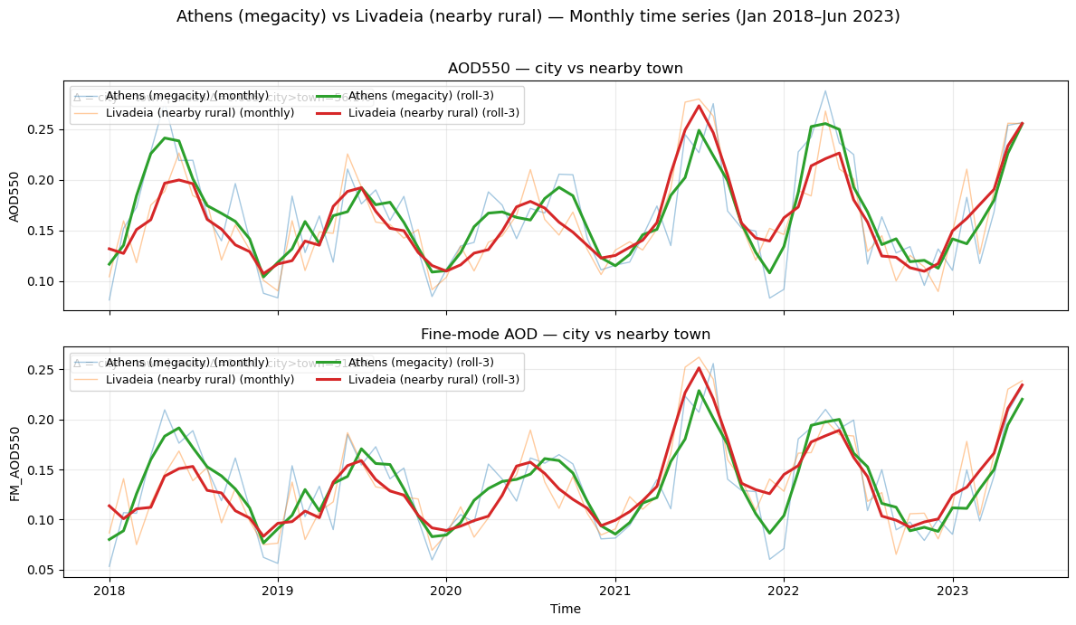
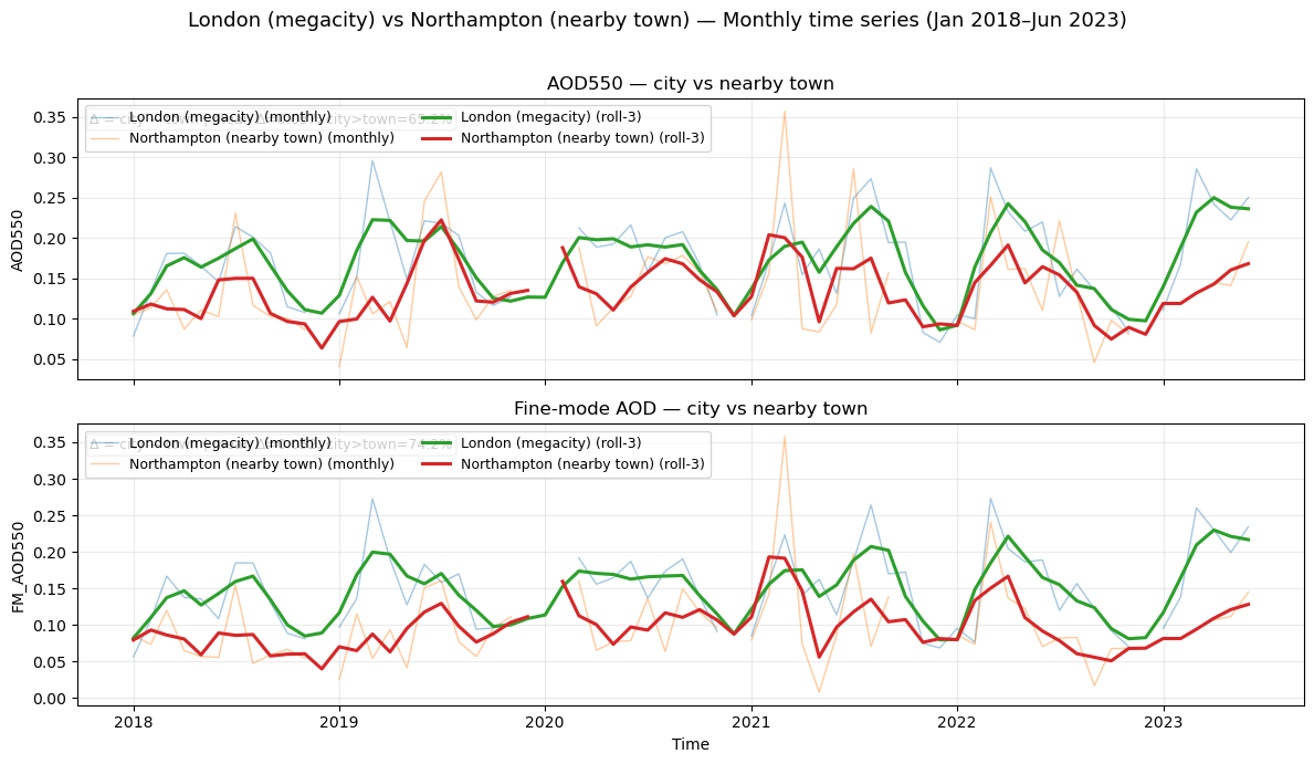
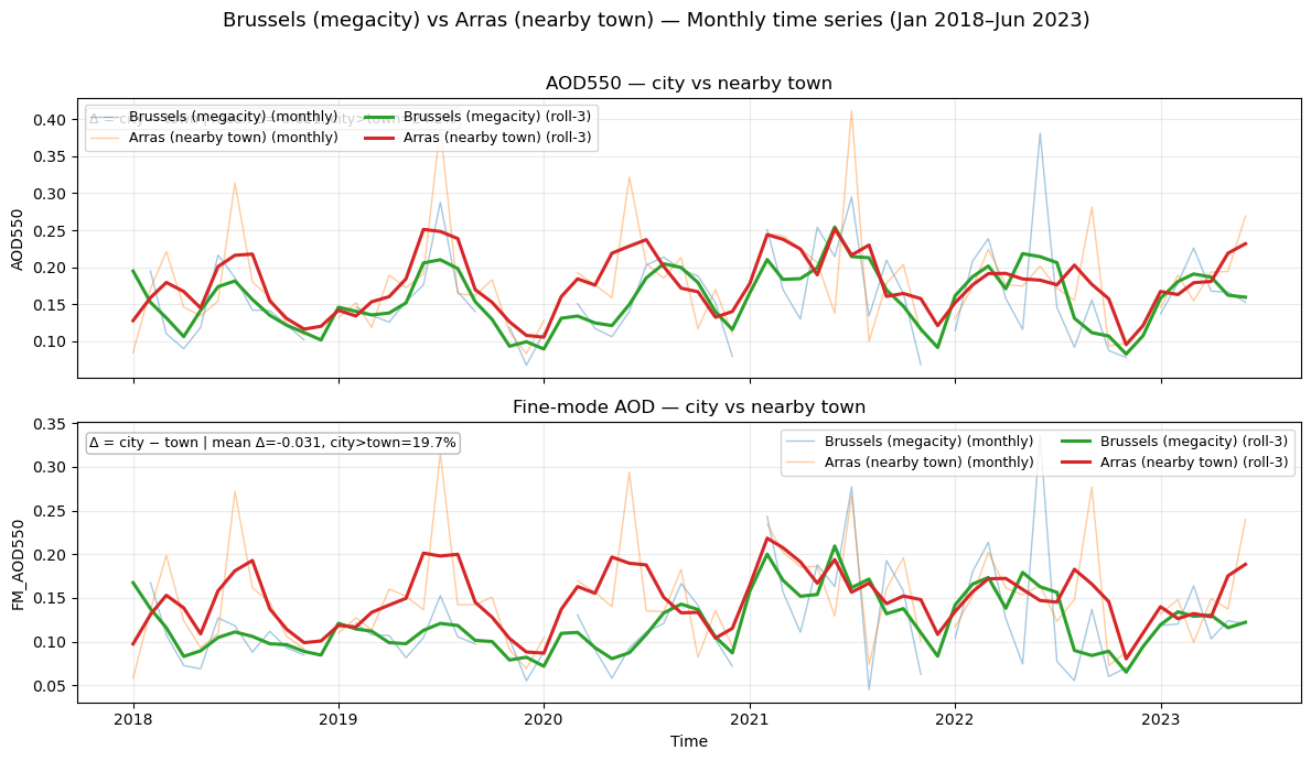
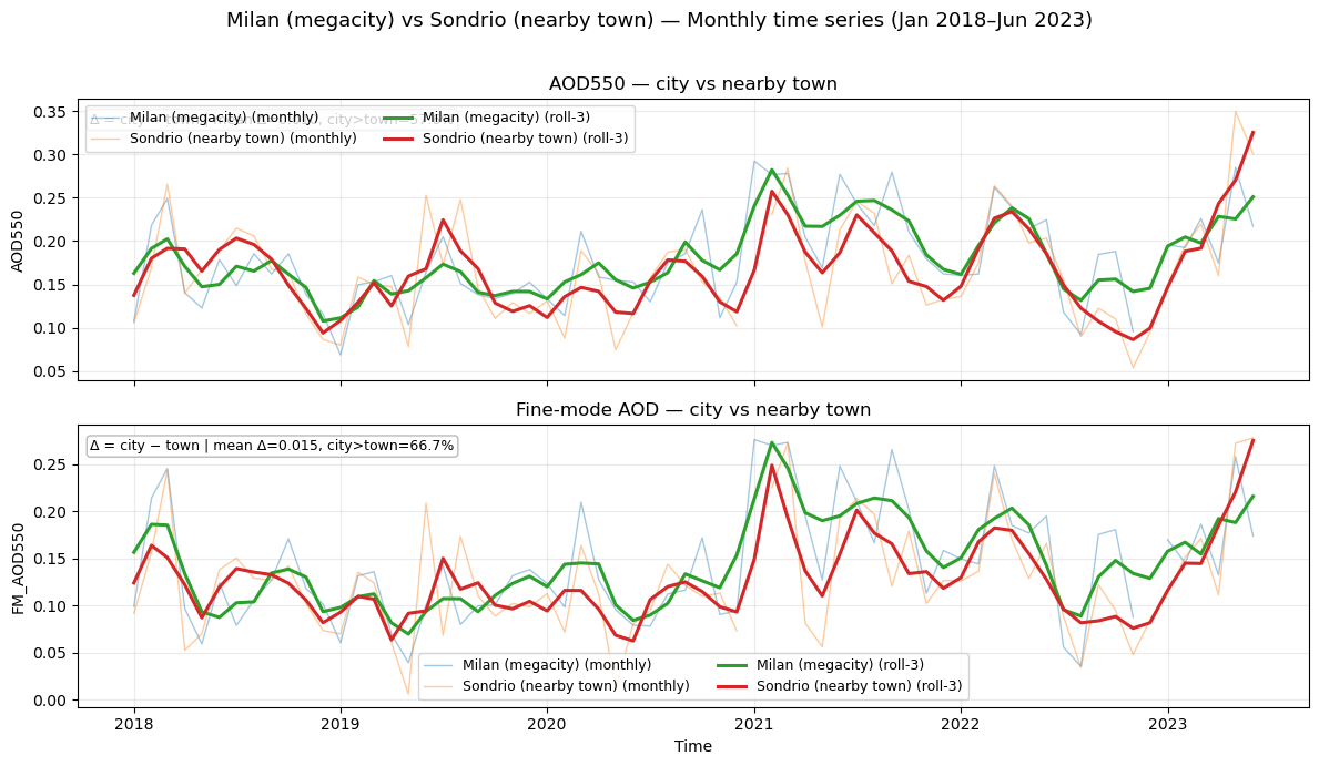
Figure 1. Monthly AOD550 and FM_AOD550 time series for Athens and Livadeia from January 2018 to June 2023. Thin lines show monthly values and thick lines show the 3-month rolling mean.

The Athens–Livadeia comparison shows that both locations follow very similar seasonal variability in AOD550 and FM_AOD550. Peaks and minima generally occur at the same time, suggesting that the signal is largely controlled by regional aerosol conditions rather than only local urban emissions from Athens. The rolling mean shows some periods when Athens is higher than Livadeia, but the separation is not persistent throughout the full period. This indicates that, for this pair, the 1° SLSTR product captures regional aerosol variability more clearly than a stable city-scale hotspot signal.

Seasonal AOD and FM-AOD maps with urban/background markers#

Each panel shows seasonal means (DJF, MAM, JJA, SON) for total AOD and fine-mode AOD. Triangles mark city AOIs their rural references. These maps provide the regional context for the urban–rural time-series and enhancement analyses.

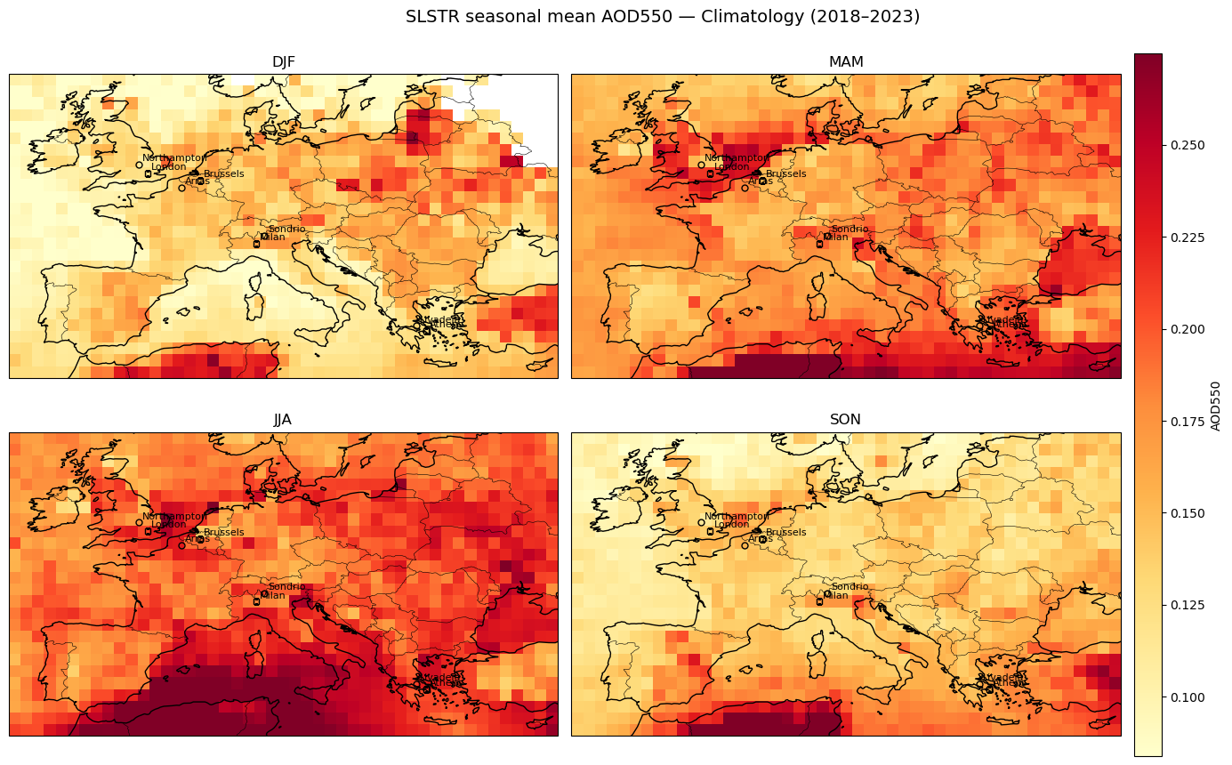
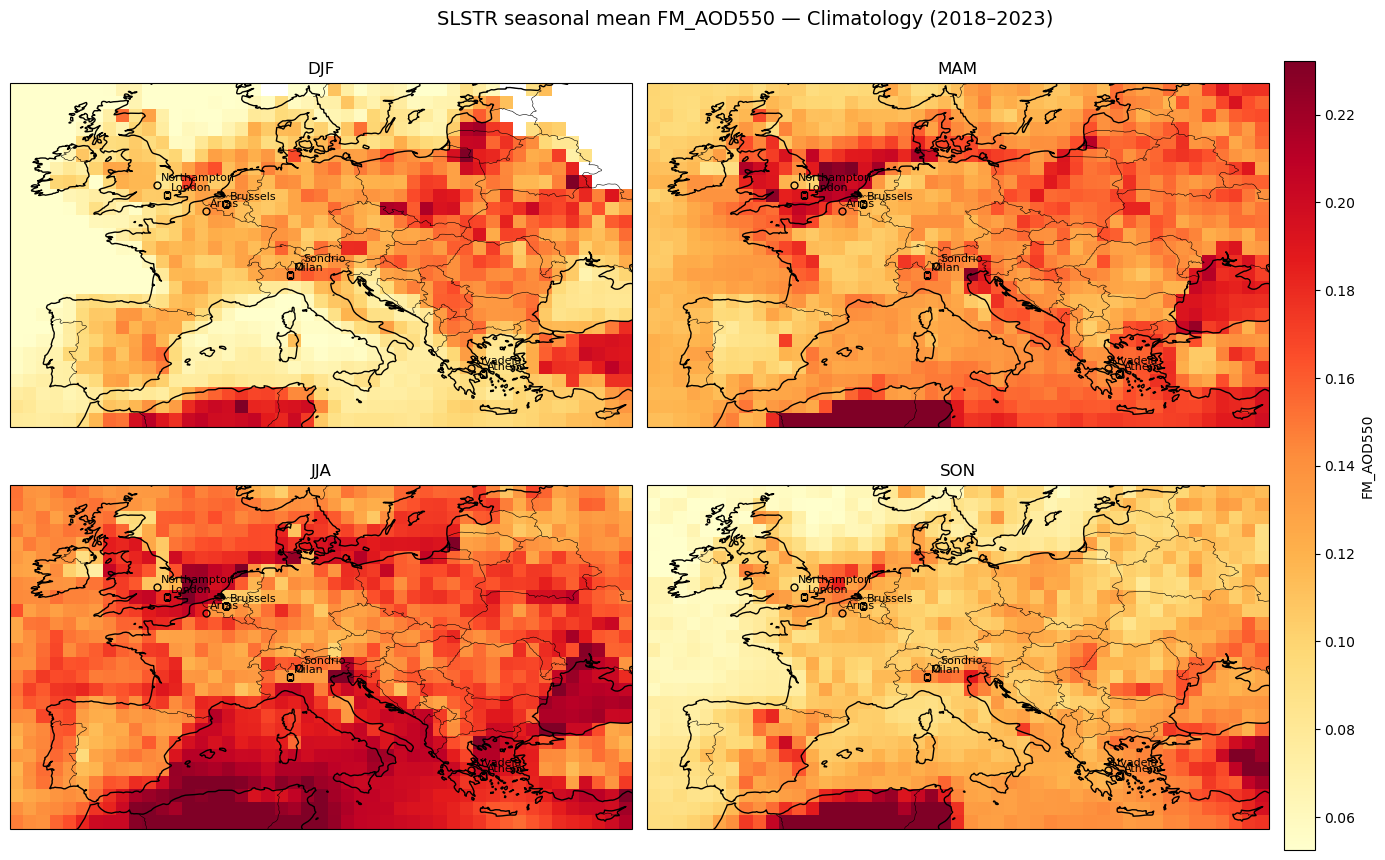
../../_images/60fc343d1edb4d04c34f0f6c48d1efa1bef5baecbb93f3cb40f9929bcea2d321.png

../../_images/6e6a0fa18f384a45f1ab7f7d956599c37d24221375fe7557c71a8fb3f0f6f09b.png

Figure 2. Seasonal AOD and Fine-Mode AOD (550 nm) over the Eastern Mediterranean, (Jan 2018–Jun 2023) (1°).

The seasonal maps show broad regional aerosol structures rather than isolated city-scale hotspots. In particular, elevated AOD over the North Sea and adjacent coastal regions should not be interpreted as direct evidence of local surface pollution in the underlying pixel. This signal may reflect a combination of transported continental pollution, ship emissions, sea-salt aerosol, humidity-driven aerosol growth, or elevated aerosol layers.

This highlights an important limitation of using column AOD for pollution-hotspot identification: the aerosol column observed by the satellite is not necessarily collocated with the surface emission source. Aerosols can be transported away from their source regions, and high AOD over a given pixel may reflect regional transport rather than local surface emissions.

For this reason, the maps are used here only to provide regional aerosol context. The hotspot assessment is based primarily on urban–background time series and pairwise differences. Even these comparisons are interpreted cautiously, because both the city and its background reference location may be affected by the same transported aerosol plume.

Focused seasonal map plots of AOD550 and FM_AOD550 for megacity–town pairs#

../../_images/bb21ccdadb8cd93955d3d8b4614548a95052331c36f9d6d0a2657a4de5f29a64.png

../../_images/2eece514478e1f9d0bd9f858859e1d24ae6e97ecb98d0d39d2e94541b4fc6871.png

../../_images/5ab0a09eb98b3d981a4ae0d6b78d13678b059d67eb5f63304cf3b355f0f06fcb.png

../../_images/8d5f2a76bdab72f3402adc99b44795da644fdb32d94752f9d933e64b17f836f1.png

../../_images/94a5d49481b78541c851ed3219782d25fcb4b1f849f0c0e5794404abf96cc8bc.png

../../_images/e1d266a1b1a56880df250ef81099a791fb6ae3a3b6fe5c5805eedddb1c0018ed.png

../../_images/a225744d5b0d055530430d988935795c1b3ca13828f88443d810b891c09ed68f.png

../../_images/f26315a461d5201af283d4bd4a2fc111032814ebe98edd43b2a2eae5c8ebbd6e.png

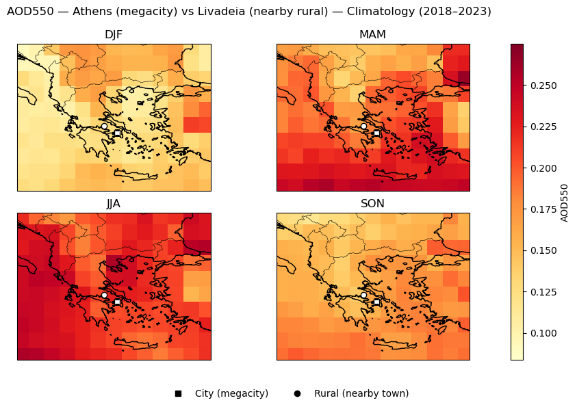
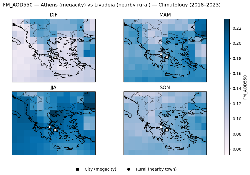
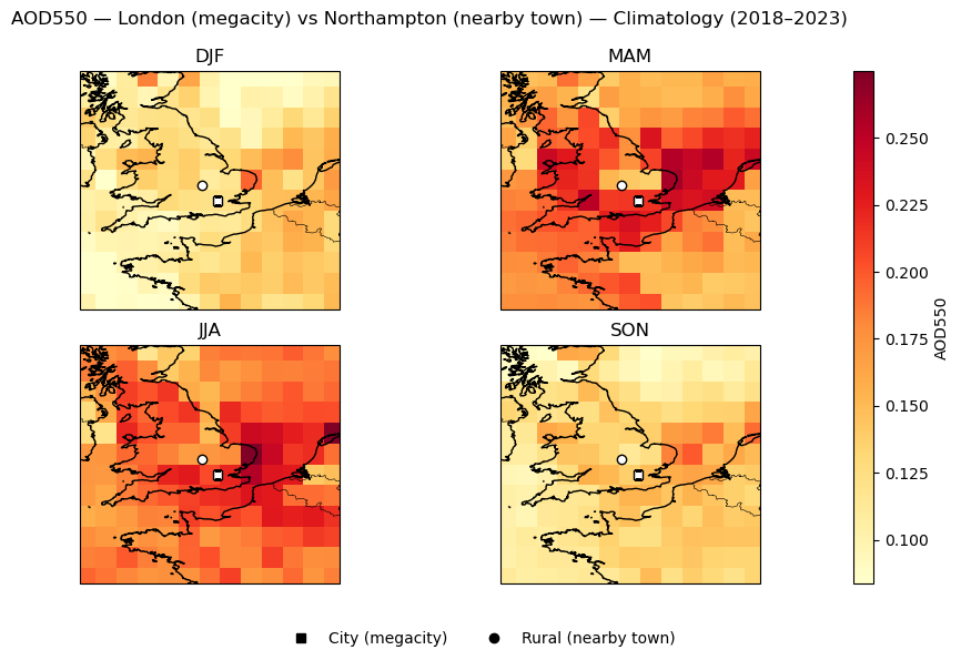
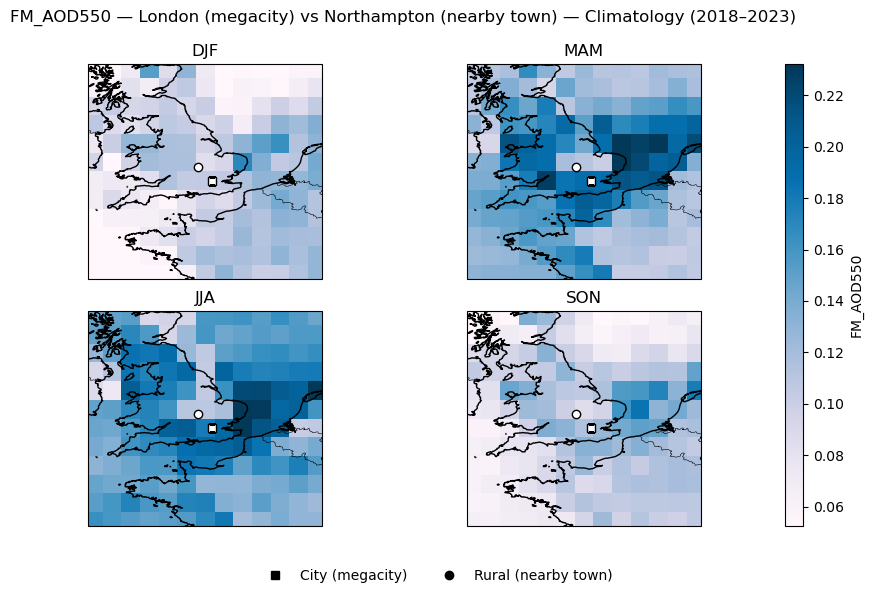
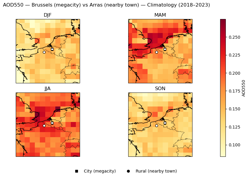
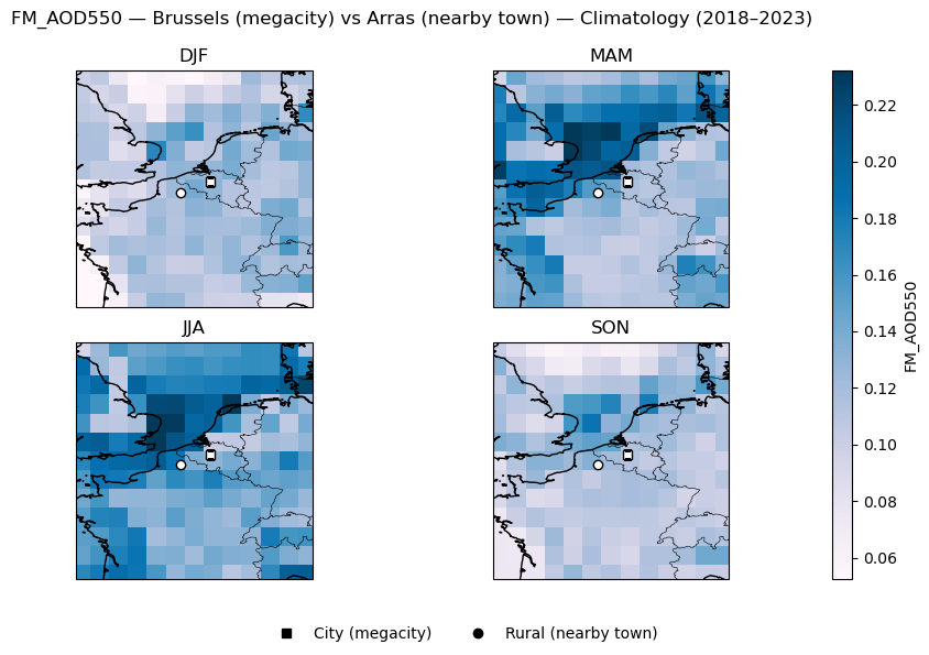
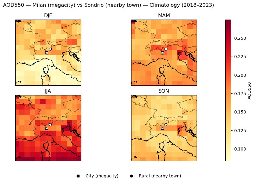
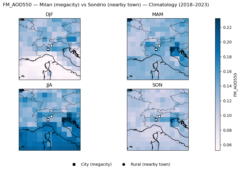
Figure 3. Focused seasonal map plots of AOD550 and FM_AOD550 for megacity–town pairs.

Take-Home Messages#

Seasonal and regional aerosol variability frequently dominates over localized city-to-city differences. In several paired cases, the large metropolitan area and the smaller reference town exhibit highly synchronized peaks in both total AOD and fine-mode AOD, underscoring the strong influence of regional-scale atmospheric episodes over local signals.
Fine-mode AOD does not consistently yield higher values over all major urban hotspots. This highlights the inherent physical challenge of utilizing satellite column-integrated AOD as a direct proxy for near-surface, ground-level pollution.
Interpreting urban aerosol contrasts requires extreme caution. Local anthropogenic signals are easily masked or redistributed by meteorology, vertical aerosol stratification, atmospheric dilution, dispersion, and the spatial averaging of the product. For this reason, comparing large metropolitan areas with nearby smaller cities, rather than with open rural fields, provides a more physically sound and sensitive framework to test the instrument’s capacity to isolate localized urban emissions against a shared regional background.
In this assessment, the smaller town of Northampton serves as the localized urban background reference for London. A brief data gap occurred for Northampton during late 2019 and early 2020 due to the unavailability of valid monthly SLSTR AOD data. These specific months were excluded from the pairwise statistics without compromising the consistency of overall seasonal analysis.
The elevated AOD patterns systematically observed over maritime sectors like the North Sea demonstrate that high column loading cannot be automatically attributed to localized surface pollution. These features often reflect transported continental plumes, shipping emissions, biomass or marine aerosols, or humidity effects. This does not invalidate the analysis, but it defines its boundaries: the satellite product is highly effective for mapping macro-regional aerosol loading, whereas robust mapping of localized urban surface hotspots requires complementary tools such as ground-based PM monitoring, emission inventories, and chemical transport modeling.
Overall, the 1° SLSTR AOD product can capture broad regional and seasonal aerosol-loading patterns over Europe, but its ability to distinguish individual urban pollution hotspots from nearby background areas is limited and strongly case-dependent. Some contrasts are visible, for example in selected seasons or pairs, but they are not persistent across all cities or variables. Therefore, SLSTR AOD is useful as a regional column-aerosol indicator, but it should not be used alone as a direct proxy for local near-surface urban pollution.

ℹ️ If you want to know more#

Key Resources#

• Aerosol properties gridded data from 1995 to present derived from satellite observations:

https://cds.climate.copernicus.eu/datasets/satellite-aerosol-properties?tab=overview

Code libraries used:

• C3S EQC custom function, c3s_eqc_automatic_quality_control, prepared by B-Open

References#

[1] Hoff, R. M., & Christopher, S. A. (2009). Remote sensing of particulate pollution from space: have we reached the promised land? Journal of the Air & Waste Management Association, 59(6), 645–675. https://pubmed.ncbi.nlm.nih.gov/19603734/

[2] Air pollution: Nearly everyone in Europe is breathing bad air — Deutsche Welle (via Copernicus Health Hub)