Please note that this repository is used for development and review, so quality assessments should be considered work in progress until they are merged into the main branch

1.2.1. Assessment of spatial coverage of SLSTR AOD (1°) for monitoring the spatial variability of wildfire-related AOD in Canada and Australia (2018–2023)

 

Production date: 30-09-2024

Produced by: Consiglio Nazionale delle Ricerche (CNR- Fabio Madonna and Faezeh Karimian.)

🌍 Use case: AOD Increase due to Wildfires from Satellite Observations

❓ Quality assessment questions

• Can satellite AOD data consistently detect seasonal wildfire-driven aerosol peaks?

• Is the spatial coverage of SLSTR AOD (1°) sufficient to study the spatial variability of wildfire-related AOD?

In the context of climate change and increasing wildfire activity, understanding the spatial and temporal distribution of aerosols from biomass burning is essential for assessing their environmental and climatic impacts. Seasonal variations in Aerosol Optical Depth (AOD) are strongly influenced by large-scale wildfires, such as those recently observed in Canada and Australia, which can inject smoke into the upper troposphere and even the lower stratosphere, with consequences for air quality, radiative forcing, and atmospheric circulation [1], [2], [3]. However, uncertainties in satellite data, including temporal consistency and retrieval sensitivity under dense smoke conditions, may affect the accuracy of such assessments [1].

The dataset analyzed is the Climate Data Store (CDS) AOD product derived from the SLSTR instrument aboard Sentinel-3, offering monthly gridded AOD values at 550 nm and ~1° spatial resolution in NetCDF format, covering the period 2018–2023. The core objective is to evaluate whether satellite observations can reliably detect the dynamics of aerosol emissions and transport linked to major fire events.

Here, the ability of SLSTR data to monitor fire-driven AOD variability is investigated in regions highly affected by wildfires, focusing on extreme fire seasons in Canada and Australia. The analysis considers both the seasonal patterns and the intensity of episodic events, aiming to determine whether current satellite-based products provide sufficient spatial and temporal resolution for reliable monitoring.

The results show periods of enhanced AOD during known wildfire seasons in the selected case studies. The analysis highlights the temporal and spatial variability of aerosol loading across the study regions, although further quantitative comparison with independent datasets would be required to assess the accuracy of these observations.

📢 Quality assessment statement

These are the key outcomes of this assessment

• The SLSTR aerosol data shows qualitative agreement with ground-based observations and Copernicus reports [5], [6] in terms of the timing of major wildfire events. However, a quantitative comparison with independent datasets is required to assess the accuracy of the retrieved AOD values.

• The AOD dataset captures periods of enhanced aerosol loading associated with documented wildfire events in the selected case studies. Nevertheless, the ability to represent the full magnitude and temporal evolution of these events remains subject to uncertainties related to spatial averaging and data availability.

• The presence of missing data for certain months (mainly during winter) in the longitude range between -100º and -80º represents a limitation of the dataset. These gaps occur close to periods of enhanced AOD and may affect the characterization of aerosol events, including their onset, duration, and peak intensity. As a result, interpretations in these regions should be treated with caution.

📋 Methodology

The methodology adopted for the analysis is split into the following steps:

Choose the data to use and set up the code

• Import all required libraries

Data Retrieval and Preparation

• Load the data and prepare the dataframe

• Define required functions

Plot and describe the results

• Plot time series for Canada and Australia

• Quantitative comparison of AOD peaks with literature

• Spatial distribution of AOD550 over Australia and Canada

• Global availability of AOD550 observations (Jan-Jul 2021)

• Spatiotemporal evolution of smoke plumes

Take-Home Messages

• Take-home message

📈 Analysis and results

Choose the data to use and set up the code

Import all required libraries

In this section, the required Python libraries are imported to handle data processing, visualization, and geospatial analysis. These include tools for working with NetCDF files, numerical computations, and plotting time series and spatial maps of aerosol optical depth (AOD).

Show code cell source

Hide code cell source

import os
import numpy as np
import pandas as pd
import xarray as xr
import matplotlib.pyplot as plt
import seaborn as sns
from scipy.ndimage import gaussian_filter
import cartopy.crs as ccrs
import cartopy.feature as cfeature

Data Retrieval and Preparation

Load the data and prepare the dataframe

In this step, the SLSTR AOD data files are loaded from local storage and combined into a single dataset for analysis. The data are stored as monthly NetCDF files, each corresponding to a specific time period.

The code loops through all available files, extracts the timestamp from each filename, and converts the data into a tabular format (dataframe). All individual datasets are then merged into a single dataframe, where missing or invalid values are handled and the data are sorted chronologically.

This structured dataframe is used for subsequent time series analysis and spatial visualization.

Show code cell source

Hide code cell source

request = {
    "time_aggregation": "monthly_average",
    "variable": ["aerosol_optical_depth"],
    "sensor_on_satellite": ["slstr_on_sentinel_3a"], 
    "algorithm": "ens",
    "version": "v2_3",
    "format": "zip"
}

Show code cell source

Hide code cell source

import xarray as xr
import os

folder_path = "./aod_data"

file_list = sorted([
    os.path.join(folder_path, f)
    for f in os.listdir(folder_path)
    if f.endswith(".nc")
])

ds = xr.open_mfdataset(file_list, combine="nested", concat_dim="time")
ds = ds.where(ds != -999.0)
times = [pd.to_datetime(os.path.basename(f)[:6], format="%Y%m") for f in file_list]
ds = ds.assign_coords(time=times)
print(ds)

<xarray.Dataset> Size: 68MB
Dimensions:                      (time: 66, latitude: 180, longitude: 360)
Coordinates:
  * time                         (time) datetime64[ns] 528B 2018-01-01 ... 20...
  * latitude                     (latitude) float32 720B -89.5 -88.5 ... 89.5
  * longitude                    (longitude) float32 1kB -179.5 -178.5 ... 179.5
Data variables:
    AOD550                       (time, latitude, longitude) float32 17MB dask.array<chunksize=(1, 180, 360), meta=np.ndarray>
    FM_AOD550                    (time, latitude, longitude) float32 17MB dask.array<chunksize=(1, 180, 360), meta=np.ndarray>
    AOD550_UNCERTAINTY_ENSEMBLE  (time, latitude, longitude) float32 17MB dask.array<chunksize=(1, 180, 360), meta=np.ndarray>
    NMEAS                        (time, latitude, longitude) float32 17MB dask.array<chunksize=(1, 180, 360), meta=np.ndarray>
Attributes: (12/18)
    Conventions:               CF-1.6
    creator_email:             thomas.popp@dlr.de
    creator_name:              German Aerospace Center, DFD
    geospatial_lat_max:        90.0
    geospatial_lat_min:        -90.0
    geospatial_lon_max:        180.0
    ...                        ...
    sensor:                    SLSTR
    standard_name_vocabulary:  NetCDF Climate and Forecast (CF) Metadata Conv...
    summary:                   Level 3 aerosol properties retreived using sat...
    title:                     Ensemble aerosol product level 3
    tracking_id:               db1b02a2-a740-11ee-aafe-0050569370b0
    version:                   v2.3

Spatial and temporal definitions

To investigate the spatiotemporal variability of wildfire-driven aerosols, the dataset was filtered both temporally and geographically. A time window was defined from January 2018 to June 2023 to cover multiple fire seasons, including extreme events in Australia (2019–2020) and Canada (2021). Spatial subsetting was then applied to isolate two regions of interest: Australia (latitudes –45° to –10°, longitudes 110° to 155°) and Canada (latitudes 45° to 75°, longitudes –140° to –50°). These filters allow for a focused analysis of AOD patterns associated with wildfire activity in regions known for severe biomass burning episodes.

Show code cell source

Hide code cell source

ds = ds.sel(time=slice("2018-01-01", "2023-06-01"))

australia_ds = ds.sel(
    latitude=slice(-45, -10),
    longitude=slice(110, 155)
)
print(australia_ds)

canada_ds = ds.sel(
    latitude=slice(45, 75),
    longitude=slice(-140, -50)
)
print(canada_ds)

<xarray.Dataset> Size: 2MB
Dimensions:                      (time: 66, latitude: 35, longitude: 45)
Coordinates:
  * time                         (time) datetime64[ns] 528B 2018-01-01 ... 20...
  * latitude                     (latitude) float32 140B -44.5 -43.5 ... -10.5
  * longitude                    (longitude) float32 180B 110.5 111.5 ... 154.5
Data variables:
    AOD550                       (time, latitude, longitude) float32 416kB dask.array<chunksize=(1, 35, 45), meta=np.ndarray>
    FM_AOD550                    (time, latitude, longitude) float32 416kB dask.array<chunksize=(1, 35, 45), meta=np.ndarray>
    AOD550_UNCERTAINTY_ENSEMBLE  (time, latitude, longitude) float32 416kB dask.array<chunksize=(1, 35, 45), meta=np.ndarray>
    NMEAS                        (time, latitude, longitude) float32 416kB dask.array<chunksize=(1, 35, 45), meta=np.ndarray>
Attributes: (12/18)
    Conventions:               CF-1.6
    creator_email:             thomas.popp@dlr.de
    creator_name:              German Aerospace Center, DFD
    geospatial_lat_max:        90.0
    geospatial_lat_min:        -90.0
    geospatial_lon_max:        180.0
    ...                        ...
    sensor:                    SLSTR
    standard_name_vocabulary:  NetCDF Climate and Forecast (CF) Metadata Conv...
    summary:                   Level 3 aerosol properties retreived using sat...
    title:                     Ensemble aerosol product level 3
    tracking_id:               db1b02a2-a740-11ee-aafe-0050569370b0
    version:                   v2.3
<xarray.Dataset> Size: 3MB
Dimensions:                      (time: 66, latitude: 30, longitude: 90)
Coordinates:
  * time                         (time) datetime64[ns] 528B 2018-01-01 ... 20...
  * latitude                     (latitude) float32 120B 45.5 46.5 ... 73.5 74.5
  * longitude                    (longitude) float32 360B -139.5 ... -50.5
Data variables:
    AOD550                       (time, latitude, longitude) float32 713kB dask.array<chunksize=(1, 30, 90), meta=np.ndarray>
    FM_AOD550                    (time, latitude, longitude) float32 713kB dask.array<chunksize=(1, 30, 90), meta=np.ndarray>
    AOD550_UNCERTAINTY_ENSEMBLE  (time, latitude, longitude) float32 713kB dask.array<chunksize=(1, 30, 90), meta=np.ndarray>
    NMEAS                        (time, latitude, longitude) float32 713kB dask.array<chunksize=(1, 30, 90), meta=np.ndarray>
Attributes: (12/18)
    Conventions:               CF-1.6
    creator_email:             thomas.popp@dlr.de
    creator_name:              German Aerospace Center, DFD
    geospatial_lat_max:        90.0
    geospatial_lat_min:        -90.0
    geospatial_lon_max:        180.0
    ...                        ...
    sensor:                    SLSTR
    standard_name_vocabulary:  NetCDF Climate and Forecast (CF) Metadata Conv...
    summary:                   Level 3 aerosol properties retreived using sat...
    title:                     Ensemble aerosol product level 3
    tracking_id:               db1b02a2-a740-11ee-aafe-0050569370b0
    version:                   v2.3

Define required functions

The following functions are defined to support the analysis and visualization of SLSTR aerosol data. They are used to extract AOD values for a selected date and region, organize the data on its original latitude-longitude grid, and generate spatial maps.

The code also includes helper routines to handle missing values and to slightly smooth the mapped field in order to improve the readability of the spatial patterns without changing the original spatial coverage. Overall, these functions make it possible to consistently produce comparable maps for different wildfire events and study areas.

Show code cell source

Hide code cell source

import numpy as np
import pandas as pd
import matplotlib.pyplot as plt
from scipy.ndimage import gaussian_filter

import cartopy.crs as ccrs
import cartopy.feature as cfeature
import cartopy.io.shapereader as shpreader
from cartopy.mpl.ticker import LongitudeFormatter, LatitudeFormatter


def _fill_nearest_2d(Z, n_iter=3):
    Z = Z.copy()

    for _ in range(n_iter):
        mask = np.isnan(Z)
        if not mask.any():
            break

        Zpad = np.pad(Z, 1, mode="edge")
        nb = np.stack([
            Zpad[:-2, 1:-1],   # north
            Zpad[2:, 1:-1],    # south
            Zpad[1:-1, :-2],   # west
            Zpad[1:-1, 2:]     # east
        ])

        valid = ~np.isnan(nb)
        count = valid.sum(axis=0)
        summed = np.nansum(nb, axis=0)

        nb_mean = np.full_like(Z, np.nan, dtype=float)
        has_neighbors = count > 0
        nb_mean[has_neighbors] = summed[has_neighbors] / count[has_neighbors]

        valid_fill = mask & has_neighbors
        if not valid_fill.any():
            break

        Z[valid_fill] = nb_mean[valid_fill]

    return Z


def native_field_from_ds(ds, date, region, var="AOD550"):
    min_lon, max_lon, min_lat, max_lat = region
    date = pd.to_datetime(date)

    sub = ds[var].sel(time=date).sel(
        latitude=slice(min_lat, max_lat),
        longitude=slice(min_lon, max_lon)
    )

    if sub.size == 0:
        raise ValueError(f"No {var} on {date.date()} in {region}")

    lon = sub["longitude"].values
    lat = sub["latitude"].values
    Z = sub.values

    return lon, lat, Z


def plot_native_map(
    ds, date, region, region_name, var="AOD550",
    vmin=0.0, vmax=0.6, levels=None, smooth_sigma=0.8,
    shapefile_path=None,
    lon_step=10, lat_step=5
):
    if levels is None:
        levels = np.linspace(vmin, vmax, 13)

    lon, lat, Z = native_field_from_ds(ds, date, region, var)

    if np.isnan(Z).any():
        Z = _fill_nearest_2d(Z, n_iter=3)

    if smooth_sigma and smooth_sigma > 0:
        Z = gaussian_filter(Z, sigma=smooth_sigma)

    LON, LAT = np.meshgrid(lon, lat)

    fig = plt.figure(figsize=(10, 6))
    ax = plt.axes(projection=ccrs.PlateCarree())
    ax.set_extent(region, crs=ccrs.PlateCarree())

    cf = ax.contourf(
        LON, LAT, Z,
        levels=levels,
        cmap="coolwarm",
        vmin=vmin,
        vmax=vmax,
        extend="both",
        transform=ccrs.PlateCarree()
    )

    if shapefile_path:
        reader = shpreader.Reader(shapefile_path)
        ax.add_geometries(
            reader.geometries(),
            crs=ccrs.PlateCarree(),
            facecolor="none",
            edgecolor="black",
            linewidth=1.2
        )
    else:
        ax.add_feature(cfeature.COASTLINE.with_scale("10m"), linewidth=1.2, edgecolor="black")
        ax.add_feature(cfeature.BORDERS.with_scale("10m"), linewidth=0.6, edgecolor="gray")

    cbar = plt.colorbar(cf, ax=ax, pad=0.02, ticks=np.linspace(vmin, vmax, 7))
    cbar.set_label(var)

    min_lon, max_lon, min_lat, max_lat = region
    ax.gridlines(draw_labels=False, linewidth=0.5, color="gray", alpha=0.5, linestyle="--")

    ax.set_xticks(
        np.arange(
            np.floor(min_lon / lon_step) * lon_step,
            np.ceil(max_lon / lon_step) * lon_step + 0.1,
            lon_step
        ),
        crs=ccrs.PlateCarree()
    )
    ax.set_yticks(
        np.arange(
            np.floor(min_lat / lat_step) * lat_step,
            np.ceil(max_lat / lat_step) * lat_step + 0.1,
            lat_step
        ),
        crs=ccrs.PlateCarree()
    )

    ax.xaxis.set_major_formatter(
        LongitudeFormatter(number_format=".0f", degree_symbol="°", direction_label=False)
    )
    ax.yaxis.set_major_formatter(
        LatitudeFormatter(number_format=".0f", degree_symbol="°", direction_label=False)
    )

    ax.set_title(f"{var} - {region_name} - {pd.to_datetime(date).date()}")
    plt.tight_layout()
    plt.show()

Plot and describe the results

Plot time series for Canada an Australia

The following code generates a time series of the monthly mean Aerosol Optical Depth (AOD550) for Australia and Canada over the study period (2018–2023).

For each region, the AOD values are averaged over all grid points for each month, producing a single representative value per time step. This allows comparison of temporal variability and identification of seasonal patterns and extreme aerosol events, particularly those associated with major wildfire episodes.

Show code cell source

Hide code cell source

# Compute regional mean time series
ts_aus = australia_ds["AOD550"].mean(dim=["latitude", "longitude"])
ts_can = canada_ds["AOD550"].mean(dim=["latitude", "longitude"])

# Plot time series
plt.figure(figsize=(12, 6))

plt.plot(ts_aus["time"], ts_aus, label="Australia")
plt.plot(ts_can["time"], ts_can, label="Canada")

plt.title("Mean AOD550 Time Series - Australia and Canada")
plt.xlabel("Time")
plt.ylabel("Mean AOD550")
plt.legend()
plt.grid(True)

plt.tight_layout()
plt.show()

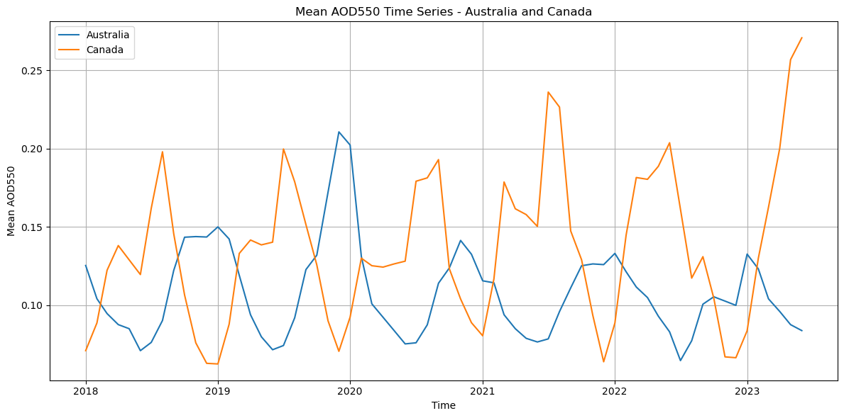
Figure 1. Time series of monthly mean AOD550 for Australia and Canada over the 2018–2023 period.

This figure shows the monthly mean Aerosol Optical Depth (AOD550) time series for Australia and Canada between 2018 and mid-2023. The time series highlights seasonal cycles and episodic peaks associated with major wildfire events, with AOD550 values consistently higher during fire seasons.

Quantitative comparison of AOD peaks with literature

To provide a quantitative perspective, the peak AOD values derived from the SLSTR dataset were compared with values reported in the literature [5] , [6].

Show code cell source

Hide code cell source

# AOD peak for Canada
max_can = ts_can.compute()
max_can_value = float(max_can.max())
max_can_time = pd.to_datetime(max_can["time"][max_can.argmax(dim="time")].values)

print(max_can_value, max_can_time)

0.2708333432674408 2023-06-01 00:00:00

Show code cell source

Hide code cell source

# # AOD peak for Australia
max_aus = ts_aus.compute()
max_aus_value = float(max_aus.max())
max_aus_time = pd.to_datetime(max_aus["time"][max_aus.argmax(dim="time")].values)

print(max_aus_value, max_aus_time)

0.21068081259727478 2019-12-01 00:00:00

Over Australia, the maximum AOD550 reaches approximately 0.21 in December 2019, corresponding to the peak of the Black Summer bushfires. In comparison, ground-based AERONET observations reported in Li et al. 2021 indicate AOD440 values ranging from ~0.15 up to 2.76 during intense smoke episodes. The lower values obtained from SLSTR are expected, as the satellite product represents spatially averaged monthly conditions, whereas AERONET measurements capture local peak concentrations. Similarly, over Canada, the maximum AOD550 reaches approximately 0.27 (June 2023), corresponding to a period of extreme wildfire activity. The timing of this peak is consistent with wildfire events reported by Copernicus Atmosphere Monitoring Service, although this source does not provide quantitative AOD values. These comparisons indicate that the SLSTR dataset captures the order of magnitude and timing of enhanced aerosol loading, although a more rigorous assessment would require direct comparison with independent datasets and the calculation of quantitative performance metrics.

Spatial distribution of AOD550 over Australia and Canada

The following code generates a spatial map of Aerosol Optical Depth (AOD550) over Australia for December 2019, corresponding to the peak of the extreme bushfire season. The data are extracted for the selected date and region, and plotted on their native grid to visualize the spatial distribution of aerosol concentrations. This allows identification of areas with enhanced AOD associated with wildfire emissions.

Show code cell source

Hide code cell source

# Australia — DEC 2019 (matches the example month with higher AOD)
plot_native_map(
    ds,
    date="2019-12-01",
    region=(110, 160, -45, -10),
    region_name="Australia",
    var="AOD550",
    vmin=0.0, vmax=0.6, smooth_sigma=0.8
)

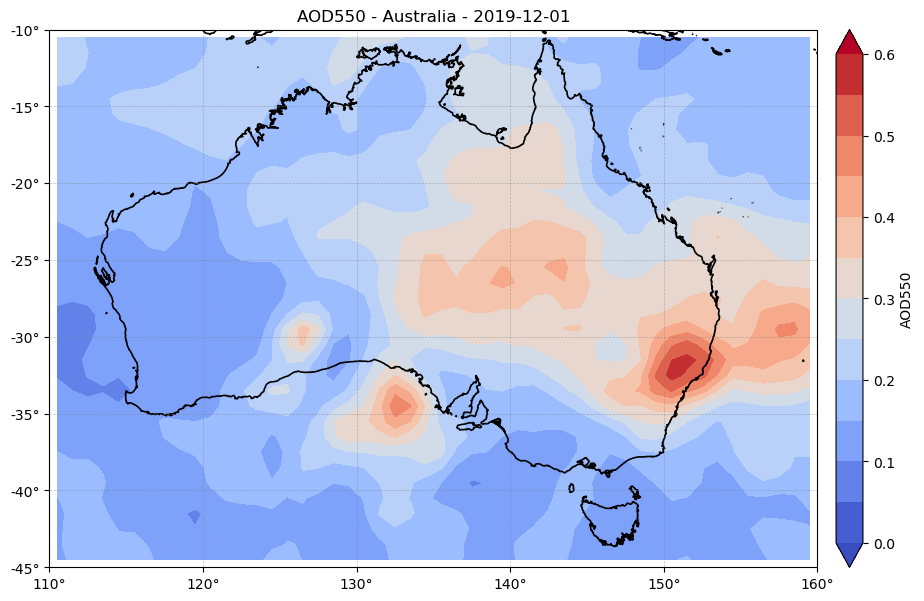
Figure 2. Spatial distribution of AOD550 over Australia on 2019-12-01, derived from SLSTR (Sentinel-3) data at ~1° resolution.

The map shows strong AOD enhancements along southeastern Australia, corresponding to the extreme bushfire season reported in the literature and in Copernicus Atmosphere Monitoring Service for late 2019. These spatial patterns are consistent with the temporal variability observed in the regional mean AOD time series (Figure 1), and help localize the areas contributing to the observed aerosol increase. [6].

The following code generates a spatial map of Aerosol Optical Depth (AOD550) over Canada for July 2021, corresponding to a period of intense wildfire activity. The data are extracted for the selected date and region, and plotted on their native grid to visualize the spatial distribution of aerosol concentrations. This enables the identification of regions affected by elevated AOD associated with wildfire smoke.

Show code cell source

Hide code cell source

# Canada — JUL 2021
plot_native_map(
    ds,
    date="2021-07-01",
    region=(-140, -50, 45, 75),
    region_name="Canada",
    var="AOD550",
    vmin=0.0, vmax=0.6, smooth_sigma=0.8
)

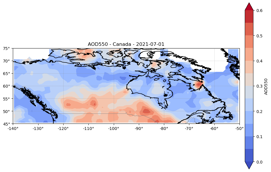
Figure 3. Spatial distribution of AOD550 over Canada on 2021-07-01, derived from SLSTR (Sentinel-3) data at ~1° resolution.

The map highlights pronounced AOD enhancements over regions in central and western Canada, consistent with wildfire smoke plumes reported in the literature for this period. These elevated aerosol levels match the temporal peaks shown in Figure 1 and align with documented fire outbreaks in governmental and scientific fire records [5].

Global availability of AOD550 observations (Jan-Jul 2021)

The following figure shows the spatial coverage of AOD550 observations used in the analysis for two selected periods in 2021. The objective is to assess the availability and continuity of the dataset across regions and time.

Show code cell source

Hide code cell source

ds_sel = ds.sel(
    time=slice("2021-01-01", "2021-07-31"),
)


aod = ds_sel["AOD550"]


aod = aod.where(aod != -999.0)


mean_map = aod.mean(dim="time")


lats = mean_map["latitude"].values
lons = mean_map["longitude"].values
Z = mean_map.values


vmin, vmax = 0.0, 0.8
levels = np.arange(vmin, vmax + 0.1, 0.1)

fig = plt.figure(figsize=(16, 9))
ax = plt.axes(projection=ccrs.PlateCarree())
ax.set_extent([-180, 180, -90, 90], crs=ccrs.PlateCarree())

LON, LAT = np.meshgrid(lons, lats)

mesh = ax.pcolormesh(
    LON, LAT, Z,
    cmap='coolwarm',
    vmin=vmin,
    vmax=vmax,
    transform=ccrs.PlateCarree(),
    shading='auto'
)

ax.coastlines(resolution='110m', linewidth=1, color='black')
ax.add_feature(cfeature.BORDERS, linewidth=0.5, edgecolor='gray')

ax.plot([110,160,160,110,110], [-45,-45,-10,-10,-45],
        color='black', linewidth=2, linestyle='--', transform=ccrs.PlateCarree())
ax.text(120, -12, "Australia", transform=ccrs.PlateCarree())

ax.plot([-140,-50,-50,-140,-140], [45,45,75,75,45],
        color='black', linewidth=2, linestyle='--', transform=ccrs.PlateCarree())
ax.text(-130, 72, "Canada", transform=ccrs.PlateCarree())

cbar = plt.colorbar(mesh, ax=ax, orientation='vertical', shrink=0.8, ticks=levels)
cbar.set_label("Mean AOD550", fontsize=14)
ax.set_title("Global Mean AOD550 (Jan–Jul 2021)", fontsize=18)

ax.set_xlabel("Longitude", fontsize=14)
ax.set_ylabel("Latitude", fontsize=14)

gl = ax.gridlines(draw_labels=True, linewidth=0.5, color="gray", alpha=0.5, linestyle="--")
gl.top_labels = False
gl.right_labels = False

plt.tight_layout()
plt.show()

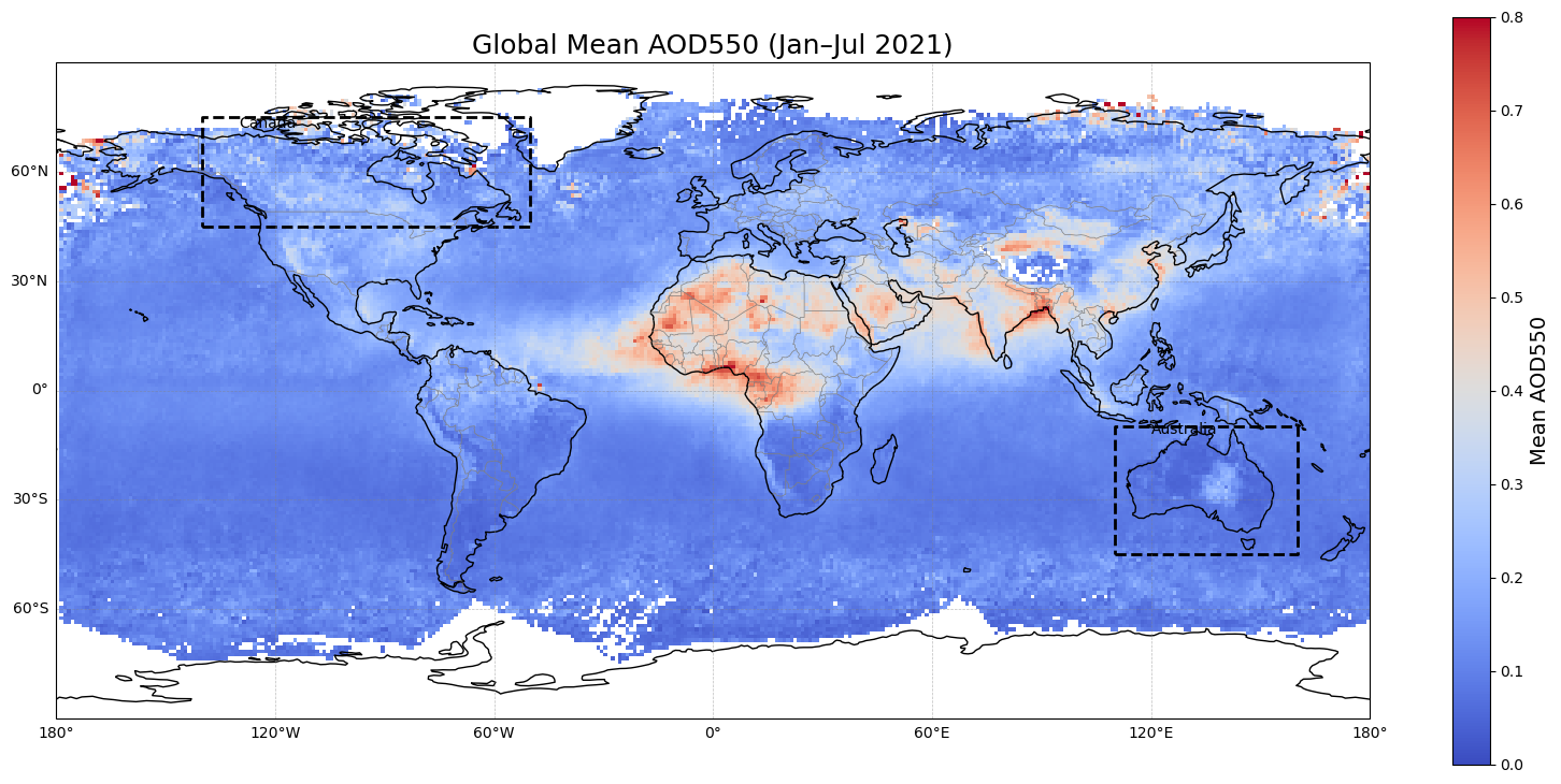
Figure 4. Global distribution of mean AOD550 for January–July 2021. White or missing areas indicate regions with no valid observations. Dashed boxes highlight the Canada and Australia study regions.

The figure highlights the spatial distribution of AOD550 observations used in this analysis and reveals that data coverage is not uniform across regions. While large areas exhibit continuous availability, several regions show partial or missing data, particularly at higher latitudes and in parts of the Southern Hemisphere.

Spatiotemporal evolution of smoke-plumes

The following code examines the spatiotemporal evolution of aerosol plumes between January and July 2021 in the latitude band 40ºN-90ºN. The data are first filtered to the study region and period, then averaged by time and longitude to produce a longitude-time diagram. This representation makes it possible to track how elevated AOD values evolve over time and spread across longitudes, helping to identify the development and transport of wildfire smoke plumes during the Canadian fire season.

Show code cell source

Hide code cell source

# Select latitude band and time period
ds_2021 = ds.sel(
    latitude=slice(40, 90),
    time=slice("2021-01-01", "2021-07-01")
)

# Extract AOD and average over latitude to build a longitude-time curtain
curtain_2021 = ds_2021["AOD550"].where(ds_2021["AOD550"] != -999.0).mean(dim="latitude")

vmin, vmax = 0.0, 0.3
levels = np.arange(vmin, vmax + 0.1, 0.1)

fig, ax = plt.subplots(figsize=(14, 6))

c = ax.imshow(
    curtain_2021.values,
    aspect="auto",
    cmap="coolwarm",
    vmin=vmin,
    vmax=vmax,
    extent=[
        curtain_2021["longitude"].min().item(),
        curtain_2021["longitude"].max().item(),
        curtain_2021["time"].max().values.astype("datetime64[D]").astype(int),
        curtain_2021["time"].min().values.astype("datetime64[D]").astype(int),
    ]
)

cbar = plt.colorbar(c, label="AOD550", ax=ax, ticks=levels)
ax.set_title("Spatiotemporal Evolution of Smoke Plumes (40°N-90°N)\nJan-Jul 2021")
ax.set_xlabel("Longitude")
ax.set_ylabel("Date")

ticks = pd.date_range("2021-01-01", "2021-07-01", freq="MS")
ax.set_yticks(ticks.values.astype("datetime64[D]").astype(int))
ax.set_yticklabels([d.strftime("%b %Y") for d in ticks])

plt.tight_layout()
plt.show()

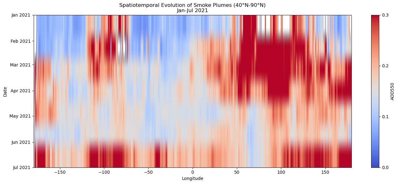
Figure 5. Hovmöller diagram showing the spatiotemporal evolution of mean AOD550 between January and July 2021 over 40°N–90°N.

Enhanced aerosol loadings appear as warm-colored bands, indicating smoke plumes transported across longitudes. These patterns align with documented wildfire activity peaks in North America during this period [6], as seen in Figures 1–3.

Take-Home Messages

• Periods of enhanced AOD identified in the SLSTR dataset occur during known wildfire seasons reported in the literature and by Copernicus Atmosphere Monitoring Service [5], [6]. However, this comparison is qualitative, and a quantitative evaluation against independent datasets would be required to assess the accuracy of the retrieved AOD values.

• Detection of wildfire-related variability: The time series analysis shows increases in AOD during periods associated with major wildfire events (e.g. December 2019 in Australia and summer 2021 in Canada). These results indicate that the dataset captures temporal variability consistent with wildfire activity, although the magnitude of the signal has not been quantitatively validated [6].

• Impact of missing data: The analysis reveals the presence of spatial and temporal gaps in AOD observations, particularly in specific longitude ranges and during certain months. These gaps may affect the identification and full characterization of aerosol events, especially when they occur close to periods of missing data.

• Spatiotemporal variability: The maps and animations illustrate changes in AOD distribution over time, highlighting the evolution of aerosol loading during selected periods. However, the identification of transport pathways remains qualitative and would require additional analysis for confirmation [6].

• Scope and limitations of the analysis: This study provides a qualitative assessment of the SLSTR AOD dataset in capturing temporal and spatial variability associated with wildfire events. A more robust evaluation would require quantitative comparison with reference datasets (e.g. AERONET or other satellite products) and the use of statistical performance metrics.

ℹ️ If you want to know more

Key Resources

• Aerosol properties gridded data from 1995 to present derived from satellite observations:

https://cds.climate.copernicus.eu/datasets/satellite-aerosol-properties?tab=overview

Code libraries used:

• C3S EQC custom function, c3s_eqc_automatic_quality_control, prepared by B-Open

References

[1] Popp, T., et al. (2016). Development, production and evaluation of aerosol climate data records from European satellite observations (Aerosol_cci). Remote Sensing, 8(5), 421.

[2] Peterson, D. A., et al. (2018). Wildfire-driven thunderstorms cause a volcano-like stratospheric injection of smoke. npj Climate and Atmospheric Science, 1, 30.

[3] Sogacheva, L., Denisselle, M., Kolmonen, P., Virtanen, T. H., & Dransfeld, S. (2022). Extended validation and evaluation of the OLCI–SLSTR Synergy aerosol product (SY_2_AOD) on Sentinel-3. Atmospheric Measurement Techniques, 15, 5289–5315.

[4] Garrigues, S., et al. (2023). Impact of assimilating NOAA VIIRS aerosol optical depth in CAMS: comparison with MODIS and analysis performance. Atmospheric Chemistry and Physics, 23, 10473–10494.

[5] Li, M., Shen, F., & Sun, X. (2021). 2019–2020 Australian bushfire air particulate pollution and impact on the South Pacific Ocean. Scientific Reports, 11, 12288.

[6] Copernicus Atmosphere Monitoring Service (CAMS). (2021). Wildfires wreaked havoc in 2021: CAMS tracked their impact.