Assessment of the consistency of surface albedo satellite data for monitoring the Caspian Sea retreat

1.2.1. Assessment of the consistency of surface albedo satellite data for monitoring the Caspian Sea retreat#

Production date: 30-09-2024

Produced by: Consiglio Nazionale delle Ricerche (CNR )

🌍 Use case: Estimating Caspian Sea retreat over time#

❓ Quality assessment question#

• Is the spatial coverage of the satellite surface albedo product sufficient to finely capture variability over the Caspian Sea?

The Caspian Sea, the world’s largest inland water body, has been experiencing a significant decline in water levels in recent decades. Sea level projections indicate a potential decrease of approximately 9 to 18 meters by the end of the century [1], posing severe risks to regional ecosystems, food security, and livelihoods, and potentially triggering socio-economic disruptions and geopolitical tensions [2], [3]. Understanding and monitoring this retreat is, therefore, a critical task. The northeastern Caspian is an area with extremely shallow bathymetry (typically less than 1 m), consisting of extensive reed beds, sandbanks, muddy shoals, and water channels [4], with surface albedo to fluctuate between 0.06 (open water) and 0.90 (snow-covered ice). In winter, ice often forms over the lake’s northernmost reaches, while the central and southern parts remain ice-free. The extreme climate of the Caspian Sea, characterized by cold winters and temperatures as low as -30°C, creates challenging working conditions for marine navigation and infrastructure. The shallow waters of the northern Caspian Sea easily freeze and are potentially covered with ice more than half a meter thick from November to late March. The Caspian Sea is currently facing an unprecedented hydrological crisis. While historical projections estimated a significant decline by the end of the century [1], recent observations indicate an alarming acceleration. Between 2005 and 2024, the sea level dropped by over 2 meters, reaching a critical low of -29.3 m in early 2024, the lowest level recorded in modern history [5]. This rapid retreat poses severe risks to regional biodiversity and maritime infrastructure, already triggering states of emergency in coastal regions like Aktau [6].

The core objective of this assessment is to determine whether the spatial coverage and resolution of the CDS Satellite Surface Albedo product (Version v2) are sufficient to capture these subtle and localized variations. Providing 10-daily, 1 km resolution broadband albedo from SPOT-VGT and PROBA-V missions, this dataset must prove its ability to discriminate between stable water bodies and the rapidly changing land-water transition zones. By integrating the Satellite Lake Water Level (Version 5.0) dataset as a reference, we examine if the 1 km spatial grid can accurately reflect physical signals associated with the retreat. Specifically, we investigate whether the product can resolve the increase in albedo caused by the exposure of the lakebed or the emergence of vegetation, as initially proposed by Chen [7]. This study evaluates if the current spatial granularity effectively captures the inter-seasonal variability of the retreating shoreline or if the increasing fragmentation of the coast demands higher-resolution monitoring tools (such as the 300 m resolution of C3S v3.1/Sentinel-3) to maintain reliable spatial coverage.

📢 Quality assessment statement#

These are the key outcomes of this assessment

The CDS 10-daily surface albedo dataset (v2) successfully captures hydrological changes linked to the Caspian Sea’s retreat.
Seasonal patterns in surface albedo are evident and consistent. Winter and spring show a decline in peak albedo values, likely due to reduced ice depth beneath the frozen lake surface and to the early ice melt. This seasonal ice loss and summer water level decline are likely influenced by rising regional temperatures and reduced snowfall [7].
Since 2016, summer albedo values have increased, coinciding with a drop in lake levels and the exposure of brighter dry lakebeds and submerged vegetation. Autumn follows a similar pattern with smaller changes.
These seasonal and interannual trends in surface albedo are consistent with recent studies showing a continued decline in Caspian Sea water levels. For example, Kostianoy and Pešić (2024) [5] report that the sea level has dropped significantly in recent years, reaching very low levels by 2024.
The estimated ~1.5 m drop in water level between 1996 and 2021 (approximately 7 cm/year), with accelerated retreat rates (~10 cm/year) from 2006 to 2021 [3], [8], is in line with the observed changes in surface albedo.
This assessment confirms that CDS (Copernicus Data Store) surface albedo can be used to monitor lake water retreat and to quantify the extent of areas where the water becomes shallow or the lake has dried up.

📋 Methodology#

This assessment has two main goals:

To evaluate the spatial and temporal consistency of satellite-derived surface albedo values with the documented lowering and retreat of water along the northern Caspian Sea coast;
To explore whether seasonal and interannual changes in surface albedo correspond to lake water retreat, using satellite-derived lake water height.

The methodology adopted for the analysis is split into the following steps:

1. Choose the data to use and set up the code

Import all the relevant packages.
Define temporal and spatial parameters

2. Data retrieval and processing

3. Plot and describe the results.

Plot Study Region (Map of Selected Area)
Time series of albedo and lake water depression relative to the Geoid
Seasonal time series panel plot of Albedo and Lake Water Height
Summer surface albedo maps and change (2006–2019)
Pixel count analysis of albedo map plots – Summer 2006 vs 2019

4. Main takeaways

📈 Analysis and results#

1. Choose the data to use and set up the code#

Import all the relevant packages#

In this section, we import all the relevant packages required to run the notebook.

Define temporal and spatial parameters#

This analysis uses surface albedo data (2006–2020) and lake water level data (v4.0) to assess whether albedo changes reflect the Caspian Sea’s retreat. The northern basin was selected due to its greater vulnerability to water level decline, as highlighted by Court et al. (2025) [4], who report that this region, with average depths of only ~5 meters, has already experienced shoreline regression exceeding 56 km and a 46% loss in surface water area between 2001 and 2024. Seasonal variations in surface albedo and water level are compared to evaluate the agreement between datasets in capturing shallow-water dynamics and lake desiccation processes.

2. Data retrieval and processing#

In this section, satellite-derived albedo and lake water height data were retrieved, processed, and prepared for analysis. Using predefined request parameters for multiple satellite sources (e.g., SPOT and PROBA), spatial and temporal datasets were downloaded using the download_and_transform function. Temporal processing involved calculating time-weighted means and spatially averaged time series. Concurrently, lake level data was retrieved and subset to the period 2006–2020. Both albedo and lake height time series were merged on a monthly basis and grouped by season and year to calculate seasonal averages. A function (get_season) was defined to map months to meteorological seasons (SON, DJF, MAM, JJA). Additionally, 10-day surface albedo data from 2006 and 2019 was downloaded to compare the spatial distribution of albedo across the study area in different years.

To ensure the reliability of the surface albedo analysis, quality control filtering was applied based on the dataset’s quality flags. Specifically, pixels flagged as having missing input data (Bit 4) or algorithm failure (Bit 7) were excluded. Bit 4 identifies cases where the input data was insufficient, such as due to cloud cover or poor observation conditions, while Bit 7 indicates that the albedo retrieval algorithm failed to produce a valid result. By removing pixels where either of these flags was set, the analysis retains only those values derived from complete and successfully processed input.

Show code cell source

Hide code cell source

maps = {}
timeseries = []

for satellite, request in requests.items():

    print(f"{satellite=}")

    maps[satellite] = download.download_and_transform(
        collection_id,
        common_request | request | {"satellite": satellite},
        chunks=chunks,
        transform_chunks=False,
        transform_func=diagnostics.time_weighted_mean,
        drop_variables=["crs"],
    )

    ds = download.download_and_transform(
        collection_id,
        common_request | request | {"satellite": satellite},
        chunks=chunks,
        transform_func=None,
        drop_variables=[],
    )

    albedo = ds["AL_BH_BB"]
    qflag = ds["QFLAG"].astype("int")

    # Apply bitmask filters for SPOT / PROBA
    input_ok = (qflag & 16) == 0        # bit 4 - missing input
    processing_ok = (qflag & 128) == 0  # bit 7 - processing issue
    valid_mask = input_ok & processing_ok

    albedo_filtered = albedo.where(valid_mask)

    # Count pixels before/after filtering
    before = albedo.count().compute().item()
    after = albedo_filtered.count().compute().item()
    print(
        f"{satellite} – valid before: {before}, after: {after}, "
        f"removed: {before - after} ({100 * (before - after) / before:.1f}%)"
    )

    # Spatial mean over the selected area
    albedo_mean = albedo_filtered.mean(dim=["latitude", "longitude"], skipna=True)

    # IMPORTANT: PROBA-V ends in June 2020
    if satellite == "proba":
        albedo_mean = albedo_mean.sel(time=slice("2014-01-01", "2020-06-30"))

    ds_filtered = albedo_mean.to_dataset(name="AL_BH_BB")
    timeseries.append(ds_filtered)

ds_timeseries = xr.concat(timeseries, dim="time").sortby("time")


# Lake data
ds_lake = download.download_and_transform(collection_id_lake, request_lake)
ds_lake_subset = ds_lake.sel(time=slice("2006-01-01", "2020-06-30"))

lake_data = ds_lake_subset["water_surface_height_above_reference_datum"]
df_lake = pd.DataFrame({
    "time": pd.to_datetime(lake_data.time.values),
    "height": lake_data.values
})
df_lake["month_time"] = df_lake["time"].dt.to_period("M").dt.to_timestamp()
df_lake["month"] = df_lake["month_time"].dt.month


# Albedo dataframe
albedo_filtered = ds_timeseries["AL_BH_BB"]
df_albedo = albedo_filtered.to_dataframe().reset_index()
df_albedo["time"] = pd.to_datetime(df_albedo["time"])
df_albedo["month_time"] = df_albedo["time"].dt.to_period("M").dt.to_timestamp()

# Optional but cleaner: one value per month
df_albedo_month = (
    df_albedo.groupby("month_time", as_index=False)["AL_BH_BB"].mean()
)

df_merged = pd.merge(df_lake, df_albedo_month, on="month_time", how="inner")
df_merged["month"] = df_merged["month_time"].dt.month


def get_season(month):
    if month in [12, 1, 2]:
        return "Winter"
    elif month in [3, 4, 5]:
        return "Spring"
    elif month in [6, 7, 8]:
        return "Summer"
    else:
        return "Autumn"

df_merged["season"] = df_merged["month"].apply(get_season)
df_merged["year"] = df_merged["month_time"].dt.year

seasonal_avg = df_merged.groupby(["year", "season"]).agg({
    "AL_BH_BB": "mean",
    "height": "mean"
}).reset_index()


# Request setup for SPOT (2006) and PROBA (2019), only for spatial maps
collection_id = "satellite-albedo"
chunks = {"year": 1}

spatial_common = {
    "format": "zip",
    "variable": "albb_bh",
    "product_version": "v2",
    "month": [f"{m:02d}" for m in range(1, 13)],
    "nominal_day": "10",
    "area": [47.5, 48.53, 45.04, 53.71],
}

spatial_requests = {
    "spot": {
        "year": ["2006"],
        "satellite": "spot",
        "sensor": "vgt",
        "horizontal_resolution": "1km",
    },
    "proba": {
        "year": ["2019"],
        "satellite": "proba",
        "sensor": "vgt",
        "horizontal_resolution": "1km",
    }
}

datasets = {}
for key, req in spatial_requests.items():
    print(f"Downloading {key} data for spatial map...")
    ds = download.download_and_transform(
        collection_id,
        spatial_common | req,
        chunks=chunks,
        transform_func=None,
        drop_variables=["crs"]
    )
    datasets[key] = ds

satellite='spot'

100%|██████████| 8/8 [00:00<00:00, 45.95it/s]
/data/common/miniforge3/envs/wp5/lib/python3.12/site-packages/earthkit/data/readers/netcdf/fieldlist.py:202: FutureWarning: In a future version of xarray the default value for data_vars will change from data_vars='all' to data_vars=None. This is likely to lead to different results when multiple datasets have matching variables with overlapping values. To opt in to new defaults and get rid of these warnings now use `set_options(use_new_combine_kwarg_defaults=True) or set data_vars explicitly.
  return xr.open_mfdataset(

spot – valid before: 15335131, after: 15329088, removed: 6043 (0.0%)
satellite='proba'

100%|██████████| 7/7 [00:00<00:00, 118.88it/s]
/data/common/miniforge3/envs/wp5/lib/python3.12/site-packages/earthkit/data/readers/netcdf/fieldlist.py:202: FutureWarning: In a future version of xarray the default value for data_vars will change from data_vars='all' to data_vars=None. This is likely to lead to different results when multiple datasets have matching variables with overlapping values. To opt in to new defaults and get rid of these warnings now use `set_options(use_new_combine_kwarg_defaults=True) or set data_vars explicitly.
  return xr.open_mfdataset(

proba – valid before: 12485442, after: 12485222, removed: 220 (0.0%)

100%|██████████| 1/1 [00:00<00:00, 36.05it/s]

Downloading spot data for spatial map...

100%|██████████| 1/1 [00:00<00:00, 56.46it/s]

Downloading proba data for spatial map...

100%|██████████| 1/1 [00:00<00:00, 93.40it/s]

3. Plot and describe the results.#

Plot Study Region (Map of Selected Area)#

To provide spatial context for the analysis, the selected study region around the Caspian Sea is visualized on a geographic map. This plot illustrates the spatial extent used for both albedo and water level data extraction. The boundaries encompass part of the northern Caspian region, an area of particular concern due to its documented vulnerability to water level decline. This vulnerability, although observed at a broader scale, is exemplified by recent findings such as those reported by Court et al. (2025), which highlight the rapid decline of the Caspian Sea level and its potential consequences for ecosystem integrity, biodiversity, and human infrastructure.

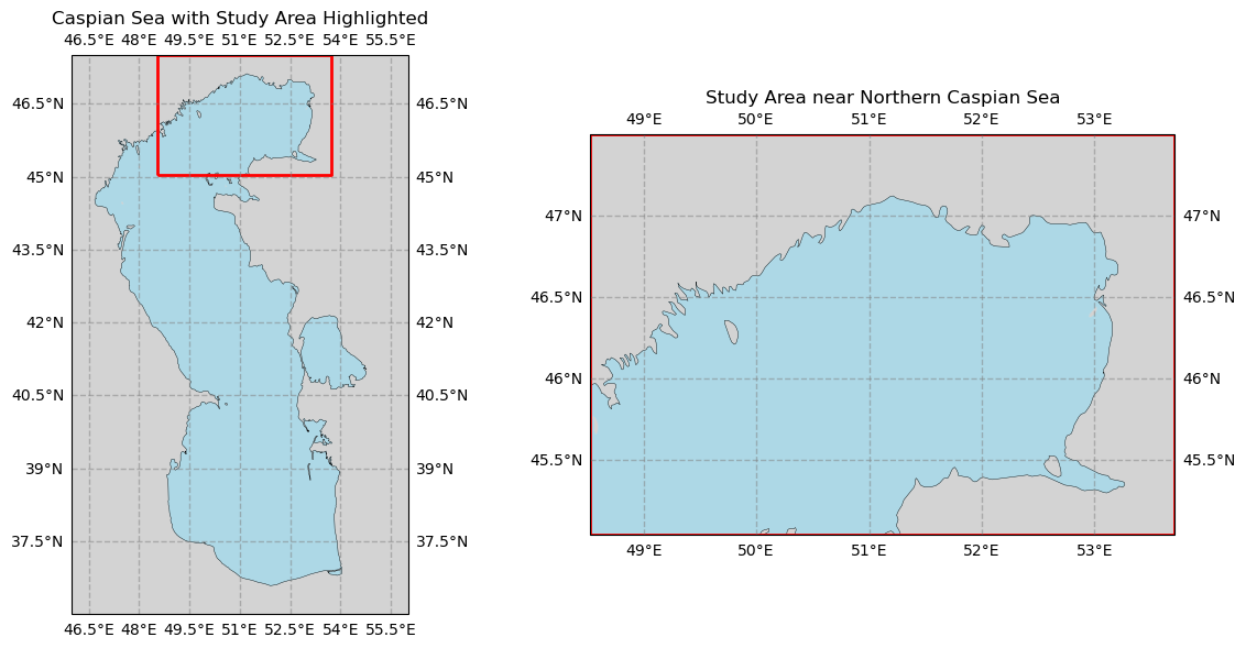
../../_images/a3319ebb59e96eae0a915188d997e037298c37bafdcf7aa0d786d674e141fa47.png

Figure 1. Maps of the Caspian Sea and the selected study region. Left: full Caspian Sea; Right: zoomed-in view of the northern section.

Time series of albedo and lake water depression relative to the Geoid#

In this section, the temporal evolution of two key environmental variables, surface albedo and lake water height, is illustrated through line plots. Monthly mean values are shown from 2006 to 2020, allowing for a direct comparison of trends and variability over time.

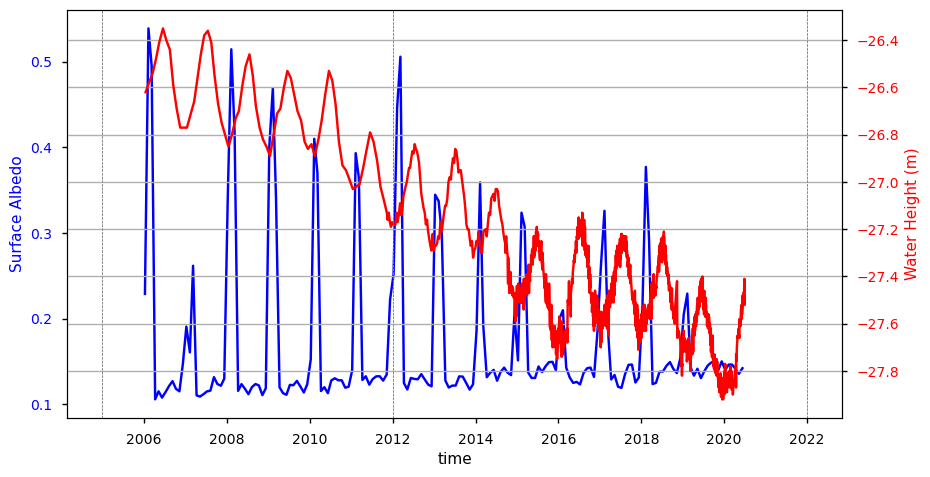
../../_images/5c6e7dd470860b659d3d0df1cd706d9b201defa2275ddfdc9f5656db0af5b30e.png

Figure 2. Time Series of Surface Albedo and Lake Water depression to the Geoid (2006–2021).

This plot shows the monthly time series of surface albedo and lake water height from 2006 to 2021. The continuous decrease in water height, combined with occasional step changes, is clearly identifiable, while surface albedo exhibits expected seasonal cycles. The albedo plot indicates that significant lake ice formation occurs in the selected region of the northern Caspian Sea during the winter months, as evidenced by the mean albedo reaching approximately 0.6. Ice extent evolution over the winter of 2006-2007 shows a smaller peak, due successive events of extensive freezing and melting throughout the season [9]. Albedo has not reached 0.6 since 2012, which suggests a less deep ice layer and less snowfall. This happens as the water’s surface height begins to decline.
Since 2016, the minimum albedo has increased, indicating that the lake water in the selected area has retreated and become shallow.

Seasonal time series panel plot of Albedo and Lake Water Height#

To highlight seasonal dynamics, the time series data for both albedo and lake height are averaged by meteorological seasons— winter (DJF), spring (MAM), summer (JJA), and autumn (SON). These are presented as a panel of subplots, with each panel representing one season across multiple years. This layout facilitates the identification of consistent seasonal patterns, anomalies, and changes in behavior over time.

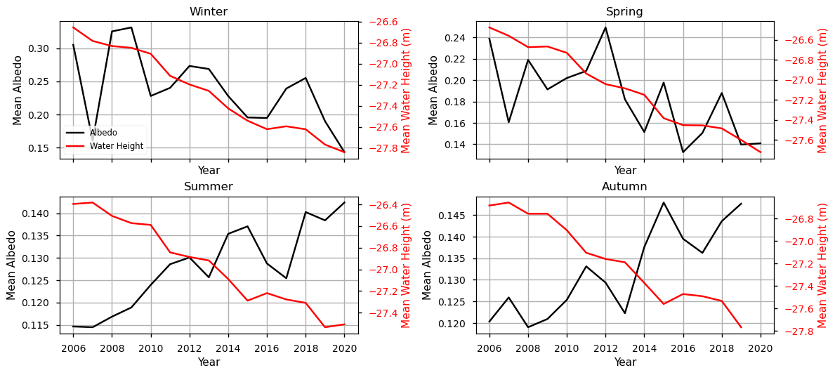
../../_images/4070dd62078aaa85ca9ad18c3987313f20e5528271d85532506a6baa93b035a5.png

Figure 3. Seasonal Average Albedo and Water Height per Year – Caspian Sea Subregion.

Water height shows a consistent decreasing trend in all seasons over the study period, indicating a long-term decline of the Caspian Sea level.
In summer and autumn, albedo displays a gradual increasing trend, which becomes more noticeable after around 2012–2014.
In contrast, winter and spring albedo are more variable, especially in the earlier years, with several pronounced peaks that may be related to changing surface or atmospheric conditions (e.g. cloud cover or snow influence).
The relationship between albedo and water level appears to be season-dependent. The clearest inverse relationship is observed in summer and autumn, where decreasing water levels are associated with increasing albedo values. This suggests that seasonal surface processes and environmental conditions influence how albedo responds to changes in water level.

Summer surface albedo maps and change (2006–2019)#

Summer spatial albedo maps are generated to better isolate the effects of seasonal water retreat. This period is particularly relevant because minimal snow cover allows for a clearer detection of lakebed exposure and vegetation changes. To further assess spatial changes in surface reflectance linked to water level decline, a difference map was produced by subtracting the summer mean albedo of 2006 from that of 2019. Positive values (shown in red) indicate areas where albedo has increased over time, which typically reflects newly exposed land, dry sediments, or vegetation expansion associated with the retreat of the lake.

Show code cell source

Hide code cell source

# Select only June, July, August
spot_summer = datasets["spot"].sel(time=datasets["spot"].time.dt.month.isin([6, 7, 8]))
proba_summer = datasets["proba"].sel(time=datasets["proba"].time.dt.month.isin([6, 7, 8]))

spot_summer_avg = spot_summer["AL_BH_BB"].mean("time")
proba_summer_avg = proba_summer["AL_BH_BB"].mean("time")
proj = ccrs.PlateCarree()

lon0, lon1 = float(spot_summer_avg.longitude.min()), float(spot_summer_avg.longitude.max())
lat0, lat1 = float(spot_summer_avg.latitude.min()),  float(spot_summer_avg.latitude.max())
pad = 0.15
extent = [lon0 - pad, lon1 + pad, lat0 - pad, lat1 + pad]

vmin = float(np.nanmin([spot_summer_avg.min(),  proba_summer_avg.min()]))
vmax = float(np.nanmax([spot_summer_avg.max(), proba_summer_avg.max()]))

fig, axes = plt.subplots(1, 2, figsize=(12, 5),
                         subplot_kw={"projection": proj},
                         constrained_layout=True)

# Figure-level title (above both panels)
fig.suptitle("Summer Mean Surface Albedo — Left: 2006 (SPOT) | Right: 2019 (PROBA)",
             fontsize=14, y=1.03)

def panel(ax, da, title):
    im = da.plot.pcolormesh(ax=ax, transform=proj, cmap="viridis",
                            vmin=vmin, vmax=vmax, add_colorbar=False)
    ax.set_title(title)
    ax.set_extent(extent, crs=proj)
    ax.coastlines(resolution="10m", linewidth=0.8)
    ax.add_feature(cfeature.BORDERS, linewidth=0.4)
    ax.add_feature(cfeature.LAKES, edgecolor="0.25", facecolor="none", linewidth=0.6)
    cs = da.plot.contour(ax=ax, transform=proj, levels=[0.14],
                         colors="white", linewidths=1.0, add_colorbar=False)
    ax.clabel(cs, fmt="0.14", inline=True, fontsize=8)
    ax.add_patch(patches.Rectangle((lon0, lat0), lon1-lon0, lat1-lat0,
                                   fill=False, ec="white", lw=1, ls="--", transform=proj))
    gl = ax.gridlines(draw_labels=True, linestyle=":", alpha=0.5)
    gl.top_labels = False
    gl.right_labels = False
    return im

_  = panel(axes[0], spot_summer_avg,  "2006 (SPOT)")
im = panel(axes[1], proba_summer_avg, "2019 (PROBA)")

# Shared colorbar for both panels
cbar = fig.colorbar(im, ax=axes, location="right", shrink=0.85, pad=0.04)
cbar.set_label("Albedo")

plt.show()

../../_images/129d75a1a4bc0324fe5d99b677192abf54a709c27115275cd8d42d5ecdbbe8b1.png

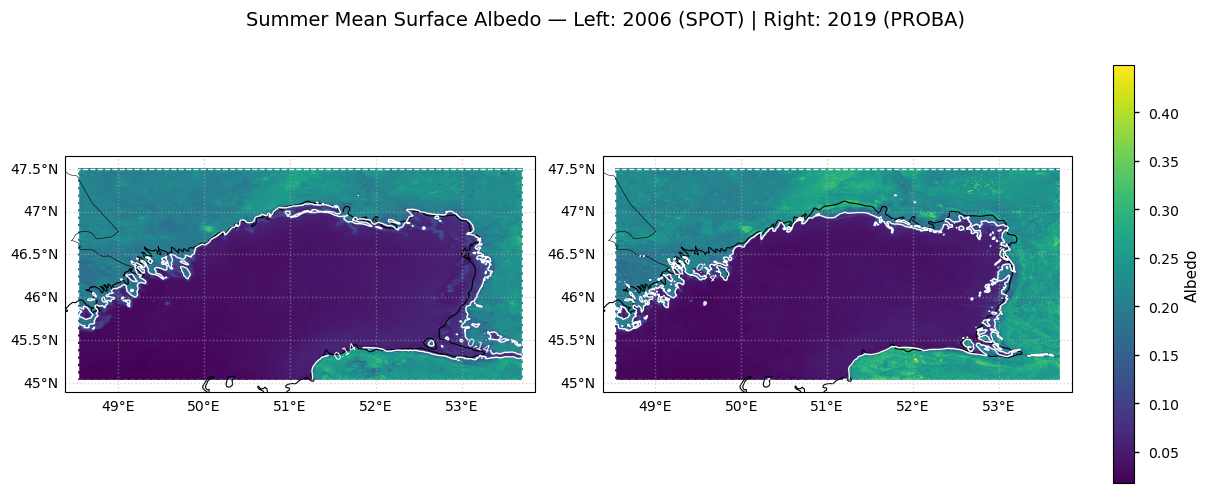
Figure 4. Summer mean albedo over the northern Caspian (NE sector) study box (1 km): Left: SPOT/VGT (2006); Right: PROBA-V (2019). Colors show broadband albedo (AL_BH_BB); the dashed rectangle is the data footprint used for the pixel analysis; coastlines outside the box provide shoreline context. The white contour (~0.14) marks a conservative threshold separating dark open water (< 0.14) from brighter, non-water surfaces.

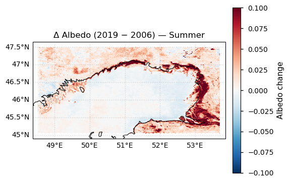
../../_images/ef62e5db719f0a7977eb4ed4cf7a611dde1101b540628e8aa21fa6d8e8c48d36.png

Figure 5. Summer albedo change (2019 − 2006) over the northern Caspian (NE sector) study box. Reds indicate brightening (higher albedo; likely exposed sediments/shallows), blues indicate darkening (lower albedo; more open water). The dashed rectangle marks the analysis footprint; coastlines provide shoreline context.

Summer spatial albedo maps are used to better capture the effects of water retreat, as minimal snow and ice allow clearer detection of lakebed exposure and vegetation changes. These maps provide a clearer view of the land–water boundary during the driest period of the year.

The comparison between 2006 and 2019 shows an increase in high-albedo areas, especially near the northern shoreline, suggesting exposure of dry sediments or vegetation due to declining water levels. To highlight these changes, a difference map (2019 − 2006) was produced.

The change map shows widespread brightening (red) along the coast, with albedo increases of up to ~0.1, indicating shoreline retreat and exposure of reflective surfaces. Smaller blue areas offshore represent localized darkening, associated with persistent open water or wetter conditions.

Pixel count analysis of albedo map plots – Summer 2006 vs 2019#

To quantitatively assess the extent of surface changes associated with lake water retreat, a pixel-based threshold analysis was performed on the summer mean albedo maps for 2006 and 2019. Based on previous studies, such as Jia Du et al. (2023), an albedo threshold of 0.14 is a reasonable lower boundary to distinguish open water surfaces (typically < 0.14) from brighter surfaces such as dry lakebeds, sediments, or emergent vegetation, which have higher reflectance [10].

Therefore, in our analysis, any pixel with albedo > 0.14 is considered as indicating non-water surface (e.g., exposed land, shallow vegetated areas, or drying sediments).

SPOT 2006 min/max/median: 0.018091666 0.34678748 0.07547708
PROBA 2019 min/max/median: 0.018063156 0.44845787 0.12332106
2006 bright>0.14: 70896/160080 (44.29%)
2019 bright>0.14: 78622/160080 (49.11%)

Applying a 0.14 albedo threshold to distinguish open water from brighter shallow-water or exposed surfaces, the analysis shows that in summer 2006 approximately 44% of the study area exceeded the threshold, increasing to about 49% by 2019. This corresponds to a +5 percentage-point increase, accompanied by a shift in median albedo from ~0.075 to ~0.123.

These results are consistent with previous studies in terms of the direction of change, indicating a reduction in open water and an increase in exposed or shallow surfaces. For example, Court et al. [4] report a substantial decrease in surface water extent over a longer period (2001–2019). However, the magnitude of change differs, which is expected given the differences in spatial coverage (our analysis focuses on a subregion of the northern Caspian), temporal sampling (two representative years versus a continuous time series), and methodological approach.

Similarly, Akbari et al. [11] document significant shoreline displacement linked to declining water levels. The observed increase in albedo, particularly in nearshore areas, is consistent with the exposure of brighter sediments and mudflats under falling lake levels.

Overall, the albedo-based analysis provides independent radiometric evidence that supports the broader geomorphological changes reported in the literature, while highlighting regional-scale variability in the magnitude of change.

4. Main takeaways#

• The CDS dataset shows high consistency with water level decline, confirming that its spatial coverage is sufficient to monitor long-term surface changes in the Northern Caspian.

• Seasonal averages show a decline in winter and especially spring albedo, likely due to reduced ice cover. Summer albedo rises noticeably after 2016, linked to falling water levels and exposure of dry or vegetated lakebed. Autumn shows a similar but smaller increase, reflecting shallower waters or surface changes from retreat.

• A difference map and seasonal averages confirm that summer surface albedo increased from 2006 to 2019, especially near the shoreline, consistent with lakebed exposure due to water retreat.

• Pixel-based analysis using an albedo threshold of 0.14 shows that the fraction of bright surfaces increased from ~44% in summer 2006 to ~49% in summer 2019 (a rise of about 6.5 percentage points, or ~15% relative). This confirms a substantial expansion of exposed or transformed surfaces consistent with shoreline retreat and lakebed exposure.

• The combination of seasonal and spatial patterns supports the use of satellite albedo data as a complementary indicator for monitoring lake retreat processes.

ℹ️ If you want to know more#

Key Resources#

Copernicus Climate Data Store (CDS)

• Surface albedo (10-daily, gridded, 1981–present) https://cds.climate.copernicus.eu/datasets/satellite-albedo?tab=overview

• Lake water levels derived from satellite altimetry (1992–present) https://cds.climate.copernicus.eu/datasets/satellite-lake-water-level?tab=overview

Code library used • c3s_eqc_automatic_quality_control – C3S EQC custom Python functions developed by B-Open

For readers interested in broader hydrological and climate context, the following resources provide useful background and complementary perspectives:

• NASA Global Water Monitor (GWM) – An overview of global surface water dynamics and satellite-based monitoring approaches: https://earth.gsfc.nasa.gov/gwm

• Climate change impacts on lakes – A comprehensive review of how climate warming affects lake systems worldwide: https://doi.org/10.1038/s43017-020-0067-5

• European State of the Climate (ESOTC) 2024 – Lakes section – Recent Copernicus assessment of lake conditions and climate-related changes: https://climate.copernicus.eu/esotc/2024/lakes

References#

[1] Nandini-Weiss, S. D., Prange, M., Arpe, K., Merkel, U., & Schulz, M. (2019). Past and future impact of the winter North Atlantic Oscillation in the Caspian Sea catchment area. International Journal of Climatology.

[2] Lahijani, H., Leroy, S. A. G., Arpe, K., & Cretaux, J. F. (2023). Caspian Sea level changes during instrumental period, its impact and forecast: A review. Earth-Science Reviews, 241, 104428.

[3] Samant, R., & Prange, M. (2023). Climate-driven 21st century Caspian Sea level decline estimated from CMIP6 projections. Communications Earth & Environment, 4(1), 357.

[4] Court, R., Lattuada, M., Shumeyko, N., Baimukanov, M., Eybatov, T., Kaidarova, A., Mamedov, E. V., Rustamov, E., Tasmagambetova, A., Prange, M., & Wilke, T. (2025). Rapid decline of Caspian Sea level threatens ecosystem integrity, biodiversity protection, and human infrastructure. Communications Earth & Environment, 6(1), 261.

[5] Kostianoy, A.G. and Pešić, V., 2024. Advances in environmental monitoring of the Caspian Sea. Ecologica Montenegrina, 76, pp.201-210.

[6] Lumbroso, D., Tsarouchi, G., Campbell, A., Davison, M., Merrien, A., Aragones, V., Kristensen, P., Li, I., Sforzi, G., Barber, D. and Wood, M., 2025. Adapting Caspian Sea ports to climate-induced water level declines: The case of Aktau.

[7] Motlagh, O. R. K., & Darand, M. (2023). Detection of land surface albedo changes over Iran using remote sensing data. SSRN Working Paper 4674763.

[8] Chen, J. L., Pekker, T., Wilson, C. R., Tapley, B. D., Kostianoy, A. G., Crétaux, J.-F., & Safarov, E. S. (2017). Long-term Caspian Sea level change. Geophysical Research Letters, 44(13), 6993–7001.

[9] Tamura-Wicks, H., Toumi, R., & Budgell, W. P. (2015). Sensitivity of Caspian sea-ice to air temperature. Quarterly Journal of the Royal Meteorological Society, 141(693), 3088–3096.

[10] Du, J., Zhou, H., Jacinthe, P. A., & Song, K. (2023). Retrieval of lake water surface albedo from Sentinel-2 remote sensing imagery. Journal of Hydrology, 617, 128904.

[11] Akbari, E., Hamzeh, S., Kakroodi, A. A., & Maanan, M. (2022). Time series analysis of the Caspian Sea shoreline in response to sea level fluctuation using remotely sensed data. Regional Studies in Marine Science, 56, 102672.

[12] Argaman, E., Keesstra, S. D., & Zeiliguer, A. (2012). Monitoring the impact of surface albedo on a saline lake in SW Russia. Land Degradation & Development, 23(4), 398–408.