

1.6.1. Completeness of ocean colour observations for biogeochemical models#
Production Date: 02-12-2024
Produced by: Chiara Volta (ENEA, Italy)
🌍 Use case: Monitoring phytoplankton dynamics in the Southern Ocean#
❓ Quality assessment question#
Is chlorophyll-a data sufficiently complete in time and space for integration into biogeochemical models?
The Ocean Colour dataset version 6.0, as produced for the Copernicus Climate Change Service (C3S), includes the two variables: mass concentration of chlorophyll-a and remote sensing reflectance (Rrs) for six wavelengths from October 1997 to present [1].
Chlorophyll-a concentration data, which are derived through specific algorithms using remote sensing reflectance (Rrs) [2], are indispensable in biogeochemical modelling as they provide inputs for models initialisation and references to calibrate biogeochemical parameters and validate models results (e.g., [3] [4] [5]). Moreover, chlorophyll-a data can be assimilated into models, enabling continuous updates with observed conditions and significantly improve their accuracy (e.g., [6]).
The dataset merges measurements carried out by six satellite sensors [1]: SeaWiFS, MERIS, MODIS-Aqua, VIIRS, OLCI-3A and OLCI-3B. Each sensor has specific design characteristics and viewing geometry, and no sensor was operational over the whole temporal coverage of the datasets [1] [2]. Currently, only OLCI-3A and OLCI-3B are operational.
Here, the goal is to assess the completeness of the chlorophyll-a dataset at both spatial and temporal scales in the Southern Ocean.
📢 Quality assessment statement#
These are the key outcomes of this assessment
The Ocean Colour dataset version 6.0:
provides a limited representation of the spatial distribution of chlorophyll-a concentrations in the oceanic region below latitude 45.5°S, based on less than 8% of valid pixels.
offers an acceptable representation of the spatial distribution of chlorophyll-a concentrations off the southeast coast of South America, based on more than 30% of valid pixels.
requires filtering based on the availability of valid pixels when analysing chlorophyll-a temporal distribution, to reduce potential bias due to limited sampling, especially during the austral winter (May-August).
allows for the calculation of monthly chlorophyll-a trends in the Southern Ocean, although these trends should be interpreted with caution as based on less than 15% of valid pixels.
can be used for calibrating, assimilating and validating biogeochemical models in the Southern Ocean from September to April, when valid observations are more abundant.
📋 Methodology#
This notebook provides an assessment of the ability of the Ocean Colour dataset version 6.0 to represent the spatial distribution and temporal variability of chlorophyll-a concentrations in the Indian, Pacific, and Atlantic Ocean sectors of the Permanent Open Ocean Zone in the Southern Ocean by analysing the number of valid pixels available.
The analysis and results are detailed in the sections below:
1. Choose the data to use and set up the code
Import required packages
Define parameters to be analysed (time period, variables, regions) and data request
2. Transform functions and data retrieval
Define transform functions
Retrieve data for the selected variables, time period and regions
3. Mapping function and trends calculation
Define mapping function
Compute trends
4. Display and discuss results
Display results
Discussion
📈 Analysis and results#
1. Choose the data to use and set up the code#
Import required packages#
Besides the standard libraries used to manage and analyse multidimensional arrays, the C3S EQC custom functions c3s_eqc_automatic_quality_controlis imported to download data and calculate statistics.
Show code cell source
import cartopy.crs as ccrs
import matplotlib.pyplot as plt
import numpy as np
import xarray as xr
import cartopy.feature as cfeature
import matplotlib.path as mpath
from pymannkendall import original_test
import calendar
import pandas as pd
from c3s_eqc_automatic_quality_control import diagnostics, download, plot, utils
plt.style.use("seaborn-v0_8-notebook")
Define parameters to be analysed (time period, variables, regions) and data request#
The analysis performed in this notebook examines the spatial and temporal distribution of chlorophyll-a data, and corresponding valid pixels, over a 21-year period (January 2003 - December 2023), which accounts for previous EQC information (https://cds.climate.copernicus.eu/datasets/satellite-ocean-colour?tab=quality_assurance_tab) and includes only complete years. The analysis is performed over three sectors within the oceanic region in the Southern Ocean located between latitudes 47.5°S and 63.5°S (i.e., the Permanent Open Ocean Zone, POOZ) [7]. The three POOZ sectors analysed are: the Indian Ocean sector (IO_POOZ), the Pacific Ocean sector (PO_POOZ) and the Atlantic Ocean sector (AO_POOZ), which extend between longitudes 20°E and 150°E, 150°E and 70°W, and 70°W and 20°E, respectively [8].
Show code cell source
# Time period
start = "2003-01"
stop = "2023-12"

# Variable
variable = "chlor_a"
assert variable in {"chlor_a"} | {f"Rrs_{wl}" for wl in (443, 560)}

# Regions
regions_monthly = {
    "IO_POOZ": {
        "lon_slice": slice(20, 150),
        "lat_slice": slice(-47.5, -63.5),
    },
    "PO_POOZ": {
        "lon_slice": slice(150, 290),
        "lat_slice": slice(-47.5, -63.5),
    },
    "AO_POOZ": {
        "lon_slice": slice(-70, 20),
        "lat_slice": slice(-47.5, -63.5),
    },
}
regions_map = {
    "SO": {
        "lon_slice": slice(-180, 180),
        "lat_slice": slice(-47.5, -63.5),
    }
}

# Define data request
collection_id = "satellite-ocean-colour"
request = {
    "projection": "regular_latitude_longitude_grid",
    "version": "6_0",
    "format": "zip",
}
chunks = {"year": 1, "month": 1, "variable": 1}
2. Transform functions and data retrieval#
Define transform functions#
The monthly_weighted_log_mean function is defined to calculate temporal averages of chlorophyll-a concentration (mg m-3) and the percentage of corresponding valid pixels for each POOZ sector by month and year, while the weighted_log_map function is defined to compute spatial averages across the entire POOZ.
Both functions account for the varying surface area at different latitudes. Averages for chlorophyll-a concentration are computed using log-transformed daily data, and then back-transformed [9]. Daily chlorophyll-a concentrations outside the range 0.01-100 mg m-3 are excluded from the analysis [10].
Show code cell source
def monthly_weighted_log_mean(ds, variable, lon_slice, lat_slice):
    da = ds[variable]
    da = utils.regionalise(da, lon_slice=lon_slice, lat_slice=lat_slice)
    if variable == "chlor_a":
        da = da.where((da > 0.01) & (da < 1.0e2))

    valid_pixels = 100 * da.notnull().groupby("time.year").map(
        diagnostics.monthly_weighted_mean, weights=False
    )
    valid_pixels.attrs = {"long_name": "Valid Pixels", "units": "%"}

    with xr.set_options(keep_attrs=True):
        da = np.log10(da * np.cos(da["latitude"] * np.pi / 180))
        da = 10 ** da.groupby("time.year").map(
            diagnostics.monthly_weighted_mean, weights=False
        )

    ds = xr.merge([da.rename("mean"), valid_pixels.rename("valid_pixels")])
    return ds.mean(["latitude", "longitude"], keep_attrs=True)


def weighted_log_map(ds, variable, lon_slice, lat_slice):
    da = ds[variable]
    da = utils.regionalise(da, lon_slice=lon_slice, lat_slice=lat_slice)
    if variable == "chlor_a":
        da = da.where((da > 0.01) & (da < 1.0e2))

    valid_pixels = 100 * da.notnull().mean("time")
    valid_pixels.attrs = {"long_name": "Valid Pixels", "units": "%"}

    with xr.set_options(keep_attrs=True):
        da = np.log10(da * np.cos(da["latitude"] * np.pi / 180))
        da = 10 ** da.mean("time")
    return xr.merge([da.rename("mean"), valid_pixels.rename("valid_pixels")])

def postprocess(ds):
    ds["mean"].attrs.update({"long_name": "Chl-a", "units": "mg m-3"})
    ds["valid_pixels"].attrs.update({"long_name": "valid pixels", "units": "%"})
    return ds
Data retrieval#
The monthly_weighted_log_mean and weighted_log_map functions are applied to the chlorophyll-a dataset in the selected regions, and temporal and spatial averages are downloaded as two separated arrays.
Show code cell source
maps = {}
for region, slices in regions_map.items():
    requests = download.update_request_date(
        request
        | {
            "variable": "remote_sensing_reflectance"
            if variable.startswith("Rrs")
            else "mass_concentration_of_chlorophyll_a"
        },
        start=start,
        stop=stop,
        stringify_dates=True,
    )
    ds = download.download_and_transform(
        collection_id,
        requests,
        transform_func=weighted_log_map,
        transform_func_kwargs=slices | {"variable": variable},
        chunks=chunks,
        transform_chunks=False,
    )
    maps[region] = postprocess(ds)

datasets = []
for region, slices in regions_monthly.items():
    requests = download.update_request_date(
        request
        | {
            "variable": "remote_sensing_reflectance"
            if variable.startswith("Rrs")
            else "mass_concentration_of_chlorophyll_a"
        },
        start=start,
        stop=stop,
        stringify_dates=True,
    )
    ds = download.download_and_transform(
        collection_id,
        requests,
        transform_func=monthly_weighted_log_mean,
        transform_func_kwargs=slices | {"variable": variable},
        chunks=chunks,
        quiet=True,
    )
    datasets.append(postprocess(ds).expand_dims(region=[region]))
ds_monthly = xr.concat(datasets, "region")
ds_monthly = ds_monthly.assign_coords(
    month_abbr=(
        "month",
        [calendar.month_abbr[month] for month in ds_monthly["month"].values],
    )
)
3. Mapping function and trends calculation#
Define mapping function#
The plot_map function is defined to visualise the maps of average chlorophyll-a concentrations and corresponding percentages of valid pixels across the POOZ.
Show code cell source
def plot_map(ax, data, lon_data, lat_data, cmap, vmin, vmax, title, cbar_label, central_longitude=0,
                  add_circle=True, add_labels=True, title_pad=55, extend='both', add_cbar=True):
    cmap = plt.get_cmap(cmap).copy()
    ax.set_extent([-180, 180, -90, -40], ccrs.PlateCarree())
    ax.add_feature(cfeature.LAND, edgecolor='k', zorder=100)
    ax.add_feature(cfeature.OCEAN, facecolor='lightblue')
    ax.coastlines(resolution='50m')
    ax.set_title(title, pad=title_pad, fontsize=30)
    gl = ax.gridlines(crs=ccrs.PlateCarree(), draw_labels=False, linewidth=1, color='gray', alpha=0.5, linestyle='--', zorder=80)
    gl.xlocator = plt.FixedLocator(np.arange(-180, 181, 10))
    gl.ylocator = plt.FixedLocator(np.arange(-90, -40 + 1, 10))

    pcolor = ax.pcolormesh(lon_data, lat_data, data, transform=ccrs.PlateCarree(), cmap=cmap, vmin=vmin, vmax=vmax, zorder=90)

    if add_cbar:
        cbar = plt.colorbar(pcolor, ax=ax, orientation='horizontal', pad=0.08, extend=extend)
        cbar.set_label(cbar_label, fontsize=40)
        cbar.ax.tick_params(labelsize=35)

    if add_circle:
        theta = np.linspace(0, 2 * np.pi, 100)
        center, radius = [0.5, 0.5], 0.5
        verts = np.vstack([np.sin(theta), np.cos(theta)]).T
        circle = mpath.Path(verts * radius + center)
        ax.set_boundary(circle, transform=ax.transAxes)

    if add_labels:
        lon_labels = np.arange(-180, 181, 20)
        for lon in lon_labels:
            if lon == 0:
                label = '0°'
            elif lon == -180:
                label = '180°'
            elif lon == 180:
                continue
            elif lon < 0:
                label = f'{abs(lon)}°W'
            else:
                label = f'{lon}°E'
            ax.text(lon, -33, label, transform=ccrs.PlateCarree(),
                    horizontalalignment='center', verticalalignment='bottom', fontsize=25)
        sector_lines = [20, 150, -70]
    for lon in sector_lines:
        ax.plot([lon, lon], [-90, -40], color='black', transform=ccrs.PlateCarree(), linewidth=3, zorder=110)
    ax.text(85, -55, 'IO_POOZ', transform=ccrs.PlateCarree(),
                horizontalalignment='center', fontsize=30, weight= 700, color='black', zorder=120)
    ax.text(220, -55, 'PO_POOZ', transform=ccrs.PlateCarree(),
                horizontalalignment='center', fontsize=30, weight= 700, color='black', zorder=120)
    ax.text(325, -60, 'AO_POOZ', transform=ccrs.PlateCarree(),
                horizontalalignment='center', fontsize=30, weight= 700, color='black', zorder=120)
    return ax
Compute trends#
The calculate_mk_trends function is defined to calculate chlorophyll-a trends and their statistical significance for each individual month over the 21-year period analysed here in the three POOZ sectors.
Show code cell source
def calculate_mk_trends(data):
    result = original_test(data)
    return {"slope": result.slope, "p_value": result.p}

slopes = np.full((len(ds_monthly_filtered['region']), len(ds_monthly_filtered['month'])), np.nan)
p_values = np.full((len(ds_monthly_filtered['region']), len(ds_monthly_filtered['month'])), np.nan)

for i, region in enumerate(ds_monthly_filtered['region'].values):
    for j, month in enumerate(ds_monthly_filtered['month'].values):
        monthly_data = ds_monthly_filtered['chl_masked'].sel(region=region, month=month).values
        valid_data = monthly_data[~np.isnan(monthly_data)]
        if valid_data.size >= 3:
            results = calculate_mk_trends(valid_data)
            slopes[i, j] = results["slope"]
            p_values[i, j] = results["p_value"]
        else:
            slopes[i, j] = np.nan
            p_values[i, j] = np.nan
mk_trends_data = xr.Dataset(
    {
        "slope": (("region", "month"), slopes),
        "p_value": (("region", "month"), p_values)
    },
    coords={"region": ds_monthly_filtered['region'].values, "month": ds_monthly_filtered['month'].values}
)
4. Display and discuss results#
Display results#
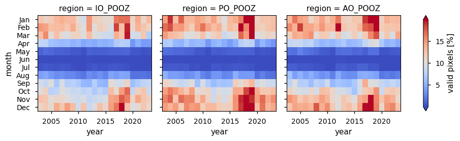
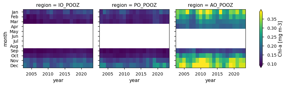
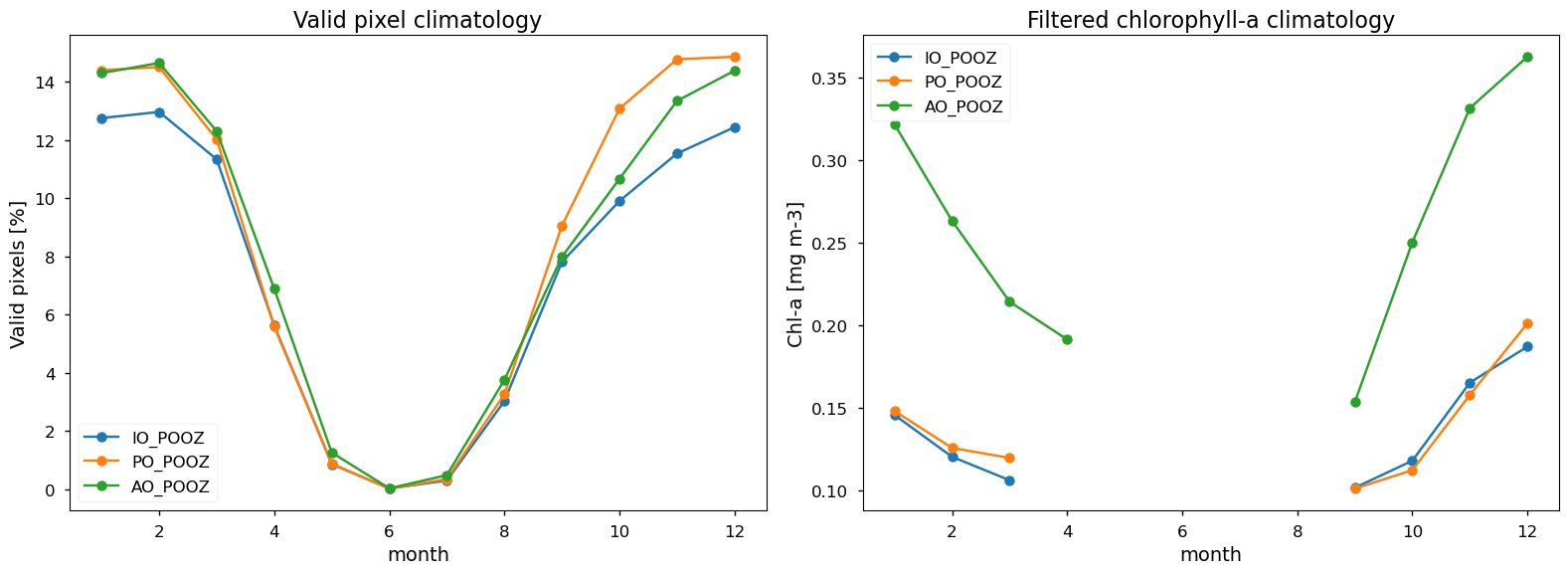
Maps showing the spatial distribution of valid pixel percentages and derived chlorophyll-a concentration in the POOZ are provided. Two sets of heatmaps are generated: one for the monthly percentage of valid chlorophyll-a pixels by POOZ sector, and another for the monthly chlorophyll-a concentrations. Here, chlorophyll-a data are displayed only when data coverage meets or exceeds the 21-year mean percentage of valid pixels across the POOZ (≈8%; see Discussion), and are referred to as filtered chlorophyll-a. Monthly climatologies of valid pixels and filtered chlorophyll-a concentrations are also shown. Trends in filtered chlorophyll-a and their statistical significance, calculated for each individual month over the 21-year period analysed, are summarised in a table, where statistically significant trends (p>0.05) are highlighted in bold and na indicates not enough data for trends calculations.
Show code cell source
# Display maps
fig, ax = plt.subplots(nrows=1, ncols=2, figsize=(24, 15), subplot_kw={'projection': ccrs.SouthPolarStereo()})
plot_map(ax[0], maps['SO']['mean'], maps['SO']['longitude'], maps['SO']['latitude'],
               cmap='viridis', vmin=0.0, vmax=0.4, title='', cbar_label='Chl-a (mg/m$^3$)',
              central_longitude=0, add_circle=True, add_labels=True, title_pad=55,
              extend='max', add_cbar=True)
plot_map(ax[1], maps['SO']['valid_pixels'], maps['SO']['longitude'], maps['SO']['latitude'],
               cmap='coolwarm', vmin=0.0, vmax=60, title='', cbar_label='Valid pixels (%)',
              central_longitude=0, add_circle=True, add_labels=True, title_pad=55,
              extend='max', add_cbar=True)
plt.tight_layout(rect=[0, 0, 1, 0.75])
plt.show()

# Filtering chlorophyll-a based on valid pixel coverage
valid_mask = ds_monthly["valid_pixels"] >= ds_monthly["valid_pixels"].mean()
coverage_fraction = valid_mask.sum(dim="year") / ds_monthly.sizes["year"]
location_mask = coverage_fraction >= ds_monthly["valid_pixels"].mean()/100
broadcast_mask = location_mask.broadcast_like(ds_monthly["mean"])
ds_monthly_masked = ds_monthly.where(broadcast_mask)
ds_monthly_filtered = xr.Dataset({
    "valid_pixels": ds_monthly['valid_pixels'],
    "chl_masked": ds_monthly_masked['mean']
})

# Display heatmaps
for var, da in ds_monthly_filtered.data_vars.items():
    facet = da.plot(
        col="region",
        x="year",
        y="month_abbr",
        cmap="coolwarm" if var == "valid_pixels" else "viridis",
        robust=True,
        ylim=(11.5, -0.5),
        xlim=(da["year"].min().item() - 0.5, da["year"].max().item() + 0.5),
    )
    facet.set_ylabels("month")
    plt.show()

# Display climatologies
plt.rcParams.update({
    'font.size': 14,
    'axes.titlesize': 16,
    'axes.labelsize': 14,
    'legend.fontsize': 12,
    'xtick.labelsize': 12,
    'ytick.labelsize': 12,
})
fig, axes = plt.subplots(1, 2, figsize=(16, 6), sharey=False)
(ds_monthly['valid_pixels'].sel(region='IO_POOZ')).mean(dim='year').plot(
    ax=axes[0], marker=".", label='IO_POOZ', ms=15)
(ds_monthly['valid_pixels'].sel(region='PO_POOZ')).mean(dim='year').plot(
    ax=axes[0], marker=".", label='PO_POOZ', ms=15)
(ds_monthly['valid_pixels'].sel(region='AO_POOZ')).mean(dim='year').plot(
    ax=axes[0], marker=".", label='AO_POOZ', ms=15)
axes[0].legend()
axes[0].set_title('Valid pixel climatology')
axes[0].set_ylabel('Valid pixels [%]')
(ds_monthly_masked['mean'].sel(region='IO_POOZ')).mean(dim='year').plot(
    ax=axes[1], marker=".", label='IO_POOZ', ms=15)
(ds_monthly_masked['mean'].sel(region='PO_POOZ')).mean(dim='year').plot(
    ax=axes[1], marker=".", label='PO_POOZ', ms=15)
(ds_monthly_masked['mean'].sel(region='AO_POOZ')).mean(dim='year').plot(
    ax=axes[1], marker=".", label='AO_POOZ', ms=15)
axes[1].legend()
axes[1].set_title('Filtered chlorophyll-a climatology')
axes[1].set_ylabel('Chl-a [mg m-3]')
plt.tight_layout()
plt.show()

# Display mk results
regions = mk_trends_data['region'].values
months = mk_trends_data['month'].values
month_abbreviations = [calendar.month_abbr[month] for month in months]
formatted_data = []
significance_flags = []
for i, region in enumerate(regions):
    row = []
    sig_row = []
    for j, month in enumerate(months):
        slope = mk_trends_data['slope'].values[i, j] * 1000
        p_value = mk_trends_data['p_value'].values[i, j]
        if np.isnan(slope) or np.isnan(p_value):
            row.append("na")
            sig_row.append(False)
        else:
            row.append(f"{slope:.4f}\n ({p_value:.4f})")
            sig_row.append(p_value <= 0.05)
    formatted_data.append(row)
    significance_flags.append(sig_row)
df = pd.DataFrame(formatted_data, index=regions, columns=month_abbreviations)
significance_df = pd.DataFrame(significance_flags, index=regions, columns=month_abbreviations)
styled_table = (
    df.style
    .set_caption("Filtered Chlorophyll-a Trends (μg m⁻³ month⁻¹)")
    .apply(lambda data: significance_df.replace({True: "font-weight: bold;", False: ""}), axis=None)
    .set_table_styles(
        [{'selector': 'th.col_heading', 'props': [('text-align', 'center')]}]
    )
    .set_properties(**{'text-align': 'center'})
)
styled_table

| Jan | Feb | Mar | Apr | May | Jun | Jul | Aug | Sep | Oct | Nov | Dec | |
|---|---|---|---|---|---|---|---|---|---|---|---|---|
| IO_POOZ | 1.7790 (0.0235) | 1.3479 (0.0003) | 1.0629 (0.0041) | na | na | na | na | na | 0.9638 (0.0001) | 0.6180 (0.0320) | 0.4780 (0.3812) | 1.3382 (0.1095) |
| PO_POOZ | 0.7043 (0.5661) | -0.2822 (0.4874) | 0.1760 (0.5260) | na | na | na | na | na | 0.5096 (0.0201) | 0.2187 (0.3812) | 0.8796 (0.0852) | 0.7861 (0.6077) |
| AO_POOZ | -0.1337 (1.0000) | 1.2132 (0.6077) | 0.5293 (0.4503) | 1.3570 (0.0372) | na | na | na | na | 0.1215 (0.7398) | -1.2910 (0.2906) | 1.0990 (0.4874) | -0.3304 (0.9759) |
Discussion#
Chlorophyll-a spatial distribution:
The mean availability of valid chlorophyll-a pixels over the 21-year period analysed is approximately 8% over the entire POOZ, indicating limited dataset coverage that may not fully capture the spatial variability of chlorophyll-a distribution in this region. A small difference in the number of valid pixels is observed across the three POOZ sectors: the PO_POOZ exhibits the greatest availability (9.5%), followed by the AO_POOZ (8.3%) and the IO_POOZ (7.3%). A significant number of valid pixels (above 30%) are detected off the southeastern coasts of South America. Therefore, the representation of the spatial distribution of chlorophyll-a in this area can be assumed to be more reliable than elsewhere in the POOZ.
Different average chlorophyll-a concentrations are observed in the three POOZ sectors: the AO_POOZ sector is the less oligotrophic with an average value of about 0.2 mg m-3, whereas the IO_POOZ and PO_POOZ are characterised by lower averages (0.12 and 0.14 mg m-3, respectively), confirming what reported in previous studies (e.g., [8]). While the subregional variability in terms of valid pixels likely depends on differences in sea ice extent and cloud coverage across the three POOZ sectors, differences in their average chlorophyll-a concentration are due to several key factors, such as nutrient supply through Patagonian dust deposition and/or upwelling (e.g., [11] [12] [13]).
Chlorophyll-a temporal distribution:
The monthly climatological distribution of valid chlorophyll-a pixels is in line with expectations based on their dependence on the solar zenith angle: the highest percentage (up to about 15%) is observed between November and February, when the solar zenith angle is low, then it decreases to reach its minimum (almost 0%) during the polar night months (i.e. May-July) and gradually increases again towards the end of the year. It is interesting to note that, as shown in the valid pixel heatmap, the valid percentages increased between 2017 and 2019, reaching a maximum in 2018 (up to about 24%), when the highest number of observing systems were operational (i.e., MODIS-Aqua, VIIRS, OLCI-3A, and OLCI-3B)
([1]).
Filtering chlorophyll-a data based on the availability of valid pixels allows to reduce the bias resulting from the lack of sampling at high latitudes, which leads to artefacts in the apparent seasonal cycle from ocean colour sensors [14]. However, the temporal distribution for the filtered chlorophyll-a data alignes with typical observations in the Southern Ocean, where chlorophyll-a concentrations decrease during the austral winter (e.g., [15]).
Linear trend analysis for all months in all three POOZ sectors yields to results summarised in the table, indicating an overall chlorophyll-a increase in the POOZ, consistent with previous studies (e.g., [8]; [16]). However, these trends should be interpreted with caution, as they are based on a low percentage of valid pixels (i.e., 8-15%). Including data prior to 2003 in the analysis would not change the sign of the significant chlorophyll-a trends but could affect their statistical significance.
Overall, the results indicate that the dataset remains valuable for biogeochemical calibration and validation in the Southern Ocean during months with reliable observations (September to April). In contrast, using data from the local winter (May-August), when satellite-derived chlorophyll-a concentrations have been shown to be overestimated [14], could lead to biased model parameterisation. This in turn may result in inflated estimates of primary production and carbon fluxes, as well as a misrepresentation of the ecosystem functioning, including nutrient cycling and grazing pressure. To address these issues, chlorophyll-a data should be filtered based on the availability of valid pixels used for their retrieval and corrected using in situ measurements (e.g., Argo floats, ship-based observations), or through assimilation techniques that incorporate satellite chlorophyll-a data from reliable seasons, enabling the model to estimate missing data based on physical and biogeochemical constraints.
ℹ️ If you want to know more#
Key resources#
CDS catalogue entry used in this notebook is the Ocean colour daily data from 1997 to present derived from satellite observations
Data download is from CDS
Product Documentation is available on the CDS website
Code libraries used:
C3S EQC custom functions,
c3s_eqc_automatic_quality_control, prepared by B-Open
Further readings:
Ocean Colour Monitoring Portals: CMEMS, ESA-GlobColour Project, ESA-OC-CCI, ESA-Sentinel 3, IMOS, NASA, NOAA CoastWatch
Groom, S., et al. (2019). Satellite Ocean Colour: Current Status and Future Perspective. Frontiers in Marine Science, 6.
Southern Ocean Carbon and Climate Observations and Modeling (SOCCOM)
References#
[1] Jackson, T., et al. (2023). C3S Ocean Colour Version 6.0: Product User Guide and Specification. Issue 1.1. E.U. Copernicus Climate Change Service. Document ref. WP2-FDDP-2022-04_C3S2-Lot3_PUGS-of-v6.0-OceanColour-product.
[2] Jackson, T., et al. (2022). C3S Ocean Colour Version 6.0: Algorithm Theoretical Basis Document. Issue 1.1. E.U. Copernicus Climate Change Service. Document ref. WP2-FDDP-2022-04_C3S2-Lot3_ATBD-of-v6.0-OceanColour-product.
[3] Doron, M., Brasseur, P., Brankart, J.-M., Losa, S.N., & Melet, A. (2013). Stochastic estimation of biogeochemical parameters from Globcolour ocean colour satellite data in a North Atlantic 3D ocean coupled physical–biogeochemical model. Journal of Marine Systems, 117-118, 91-95.
[4] Sammartino, M., Marullo, S., Santoleri, R., & Scardi, M. (2018). Modelling the Vertical Distribution of Phytoplankton Biomass in the Mediterranean Sea from Satellite Data: A Neural Network Approach. Remote Sensing, 10(10), 1666.
[5] Dutkiewicz, S., Hickman, A.E., Jahn, O., Henson, S., Beaulieu, C., & Monier, E. (2019) Ocean colour signature of climate change. Nature Communications, 10, 578.
[6] Pradhan, H.K., Völker, C., Losa, S. N., Bracher, A., & Nerger, L. (2019). Assimilation of global total chlorophyll OC-CCI data and its impact on individual phytoplankton fields. Journal of Geophysical Research: Oceans, 124, 470-490.
[7] Orsi, A.H., Whitworth, T., & Nowlin, W.D. (1995). On the meridional extent and fronts of the Antarctic Circumpolar Current. Deep Sea Research Part I: Oceanographic Research Papers, 42(5), 641-673.
[8] Del Castillo, C.E., Signorini, S.R., Karaköylü, E.M., & Rivero-Calle, S. (2019). Is the Southern Ocean Getting Greener? Geophysical Research Letters, 46, 6034-6040.
[9] Campbell, J.W. (1995). The lognormal distribution as a model for bio-optical variability in the sea. Journal of Geophysical Research, 100, 13237-13254.
[10] Sathyendranath, S., et al. (2019). An Ocean-Colour time series for use in climate studies: the experience of the Ocean-Colour Climate Change Initiative (OC-CCI). Sensors, 19, 4285.
[11] Sokolov, S., & Rintoul, S.R. (2007). On the relationship between fronts of the Antarctic Circumpolar Current and surface chlorophyll concentrations in the Southern Ocean, Journal of Geophysical Research, 112, C07030.
[12] Paparazzo, F.E., Crespi-Abril, A.C., Gonçalves, R.J., Barbieri, E.S., Gracia Villalobos, L.L., Solís, M.E., & Soria, G. (2018). Patagonian dust as a source of macronutrients in the Southwest Atlantic Ocean. Oceanography, 31(4), 33-39.
[13] Demasy, C., Boye, M., Lai, B., Burckel, P., Feng, Y., Losno, R., Borensztajn, S., & Besson, P. (2024). Iron dissolution from Patagonian dust in the Southern Ocean: under present and future conditions. Frontiers in Marine Science, 11, 1363088.
[14] Gregg, W.W., & Casey, N.W. (2007). Sampling biases in MODIS and SeaWiFS ocean chlorophyll data. Remote Sensing of Environment, 111(1), 25-35.
[15] Arteaga, L.A., Boss, E., Behrenfeld, M.J., Westberry, T.K., & Sarmiento, J.L. (2020). Seasonal modulation of phytoplankton biomass in the Southern Ocean. Nature Communications, 11, 5364.
[16] Venegas, R.M., Rivas, D., & Treml, E. (2025). Global climate-driven sea surface temperature and chlorophyll dynamics. Marine Environmental Research, 204, 106856