

1.3.1. Gravimetric mass balance data from satellite observations: utility analysis for mass change monitoring of the ice sheets#
Production date: 31-03-2025
Dataset version: 4.0
Produced by: Yoni Verhaegen and Philippe Huybrechts (Vrije Universiteit Brussel)
🌍 Use case: Using ice sheet mass changes as indicators for global climatic and water cycle changes in the context of the current global climate change#
❓ Quality assessment question#
“Is the dataset sufficiently consistent in terms of spatio-temporal completeness to derive multi-year trends in ice sheet mass changes and their corresponding contribution to global sea level rise?”
Ice sheets are significant contributors to current (and future) global sea-level rise, indicators of climatic changes, and key players regarding feedback mechanisms within the atmosphere, ocean, and cryosphere. Assessing ice sheet mass changes is essential for understanding these mechanisms. At present-day, the gravimetric method from satellite-based remote sensing offers one out of the three feasible ways to regularly and accurately monitor mass changes of the entire ice sheets at a regular basis (the others being the altimetric and input-output method). The “Gravimetric mass balance data for the Antarctic and Greenland ice sheets from 2003 to 2022 derived from satellite observations” dataset on the Climate Data Store (CDS) therefore provides valuable insights into the ice sheet’s mass changes. The dataset uses satellite gravimetry from the GRACE and GRACE-FO missions to detect changes in the Earth’s gravitational field. These are then translated into cumulative mass anomalies of ice above buoyancy for the grounded ice of both the Greenland (GrIS) and Antarctic (AIS) ice sheets [1, 2]. This notebook investigates whether the mass change dataset is of sufficient maturity and quality in terms of its spatio-temporal completeness (i.e. coverage and resolution) to derive multi-year trends in ice sheet mass changes and their corresponding contribution to global sea level rise. For that, we use dataset version 4.0.
📢 Quality assessment statements#
These are the key outcomes of this assessment
The ice sheet mass change dataset, making use of the GRACE(-FO) satellite missions, is a useful tool for quantifying the total ice mass change of the Greenland (GrIS) and Antarctic (AIS) ice sheets. The C3S data are presented as a time series of the ice sheet GMB data and exhibits a long temporal extent (> 20 years). The data represent mass changes aggregated from different basins or from an ice sheet-wide coverage at a (quasi) monthly temporal resolution. Since it only captures ice mass changes above buoyancy, ice mass changes from GRACE(-FO) can be directly converted to global sea level contributions, of which the dataset values agree well with values found in the literature from other methods [9, 12, 13]. The C3S GMB dataset therefore effectively captures the long-term mean, trends and variability of ice sheet mass changes and the corresponding global sea level contributions, and can thus serve as a clear indicator of global climate change and water cycle changes.
Data limitations include a coarse spatial resolution of the data acquisition and dataset itself (i.e. since there is a lack of gridded data at the pixel level of the final product, the term “spatial resolution” is actually not appropriate for this dataset), undesired signal leakage from adjacent regions (e.g. the nearby Canadian ice caps for the GrIS), and the need for complex data retrieval methods and geophysical corrections resulting in occasionally very high uncertainty values. Furthermore, data gaps exist, notably during 2017-2018 in between the transition of GRACE and its follow-up GRACE-FO. These are not flagged or filled, requiring users to manually identify missing periods. However, for linear trend estimation, gaps (even long ones) in the time series are practically irrelevant, as mass changes occurring during these gaps are still included in the subsequent solution, and secondly, there is no systematic bias between GRACE and GRACE-FO.
📋 Methodology#
Dataset description#
The total mass balance of an ice sheet is the difference between mass gained (mainly from snow accumulation) and mass lost (by ablation or solid ice discharge across the grounding line), which is the same as the net mass change of the ice sheet. Remote sensing techniques, such as the use of satellites, are an important feature to derive and study the mass changes of the ice sheets. The ice sheet mass change dataset provides monthly gravimetric mass balance (GMB) values and their uncertainty for the Greenland (GrIS) and also the Antarctic ice sheet (AIS). The data represent a time series of the cumulative mass changes (mass anomalies) of the ice above buoyancy of the ice sheets and their basins (including ice caps and glaciers) that are derived using satellite gravimetry data from the GRACE(-FO) missions. Data are available as time series for the whole ice sheet, as well as at the basin level, but no gridded data are provided. Data are available since 2002 with units in Gt (Gigatonnes). For a more detailed description of the data acquisition and processing methods, we refer to the documentation on the CDS and the ECMWF Confluence Wiki (Copernicus Knowledge Base).
The mass changes and their errors derived from GRACE(-FO) are expressed in Gt (Gigatonnes). It can also be translated into a volume, for example one Gt of water (density 1000 kg/m\(^3\)) is exactly one km\(^3\), while one Gt of ice (density 917 kg/m\(^3\)) in volume becomes 1.091 km\(^3\) of ice. GRACE(-FO) data are in fact considered to be the sum of mass changes driven by changing rates of solid ice discharge (i.e. the flux across the grounding line \(D\)) and mass changes driven by changing rates of ablation and accumulation (mainly the surface mass balance or \(SMB\)). What GRACE(-FO) actually detects are patterns of mass redistribution, indicating that a material should be redistributed (e.g. by ice dynamics or liquid discharge) in order for GRACE(-FO) to be able to detect gravity anomalies and the corresponding mass changes over certain locations. In that sense, an amount of melted ice being replaced by its mass-equivalent amount of meltwater at the same location would result in zero mass change.
The main advantage of GRACE(-FO) is that all processes directly contributing to ice sheet mass fluctuations are observed directly. Unlike the input-output method, SMB is therefore not involved explicitely in processing and it is not separated from ice flow dynamics. Moreover, gaps in the time series do not affect linear trend estimation as mass changes occurring during these gaps are still included in the subsequent solution. The main drawbacks of this technique are the large footprint of data acquisition and the fact that corrections must be made for mass redistribution in the atmosphere, ocean, soil and solid earth (e.g. glacial isostatic adjustment) in order to isolate mass changes relevant for the ice sheets.
Structure and (sub)sections#
1. Data preparation and processing
2. Quantifying Greenland and Antarctic Ice Sheet mass changes over time
3. Ice sheet mass change trends and sea level contribution over time
📈 Analysis and results#
1. Data preparation and processing#
1.1 Import packages#
First we load the packages:
Show code cell source
import fsspec
import matplotlib as mpl
import matplotlib.pyplot as plt
import matplotlib.colors as mcolors
import matplotlib.ticker as mticker
import numpy as np
import xarray as xr
from scipy.stats import linregress
from matplotlib.gridspec import GridSpec
import re
from math import ceil
import scipy.stats
import pandas as pd
import calendar
import os
from c3s_eqc_automatic_quality_control import download
plt.style.use("seaborn-v0_8-notebook")
1.2 Define parameters and download#
Then we define the parameters, i.e. for which ice sheet (or which basins of these ice sheets) we want the mass change data to be extracted:
Show code cell source
variables = ["GrIS_total", "AntIS_total"]
Then we define requests for download from the CDS and download and transform the glacier mass change data.
Show code cell source
collection_id = "satellite-ice-sheet-mass-balance"
request = {
    "variable": "all",
    "format": "zip",
}
ds = download.download_and_transform(collection_id, request)
ds = ds[variables].compute()
ds = xr.combine_by_coords([ds])
print("Downloading done.")
100%|██████████| 1/1 [00:00<00:00, 28.68it/s]
Downloading done.
1.3 Display and inspect data#
Let us inspect the data:
Show code cell source
ds
<xarray.Dataset> Size: 3kB
Dimensions:      (time: 216)
Coordinates:
  * time         (time) datetime64[ns] 2kB 2002-04-16T20:23:54.375000 ... 202...
Data variables:
    GrIS_total   (time) float32 864B 1.057e+03 1.123e+03 ... -3.762e+03
    AntIS_total  (time) float32 864B 345.6 488.9 467.3 ... -910.0 -843.2 nan
Attributes:
    Title:                GMB for Greenland and Antarctica ice sheets from th...
    institution:          DTU Space - Geodesy and Earth Observations
    reference:            Baratta et al. (2016), Groh and Horwart (2016)
    file_creation_date:   Tue May 16 09:49:32 2023
    region:               Greenland and Antarctica
    missions_used:        GRACE and and GRACE-FO
    time_coverage_start:  Apr-2002
    time_coverage_end:    Dec-2022
    Tracking_id:          ab2360a4-82d5-42f3-babb-90ce976a8a8e
    netCDF_version:       NETCDF4
    product_version:      4.0
Summary: This data set is prepared for the C3S project, and ...It is a dataset that consists of time series data, containing cumulative values of the total ice sheet mass change of, in this case, the entire Greenland Ice Sheet (GrIS_total) and the entire Antarctic Ice Sheet (AntIS_total) since 2002. Mass changes are expressed in units of Gt and the time period between two measurements is variable. Note that no gridded data are given in this dataset, and hence no spatial resolution can be derived.
1.4 Data handling and creating functions#
Let us perform some data handling before getting started with the analysis. We also define a plotting function to visualize the time series:
Show code cell source
def plot_timeseries(ds):
    # Define specific names for the first and second variables
    variable_names = {
        "first_variable_name": "Cumulative mass change of the Greenland Ice Sheet from GRACE(-FO)",
        "second_variable_name": "Cumulative mass change of the Antarctic Ice Sheet from GRACE(-FO)"
    }

    variables = list(ds.data_vars.values())
    num_vars = len(variables)

    # Determine the number of columns needed based on the number of variables
    num_cols = (num_vars + 1) // 2  # Integer division to ensure enough columns

    fig = plt.figure(figsize=(10 * num_cols, 8))
    gs = GridSpec(2, num_cols, figure=fig)

    # Convert time to pandas datetime for easy handling
    time_values = pd.to_datetime(ds["time"].values)

    for i, var in enumerate(variables):
        row = i % 2
        col = i // 2
        ax = fig.add_subplot(gs[row, col])
        var.plot(ax=ax, color='k')
        ax.set_title(f"{var.attrs.get('region', '')}")
        ax.set_xlim(np.min(ds["time"]), np.max(ds["time"]))
        ax.grid(color='#95a5a6', linestyle='-', alpha=0.25)

        # Identify large gaps and shade them
        for i in range(len(time_values) - 1):
            gap = (time_values[i + 1] - time_values[i]).days
            if gap > 35:
                ax.fill_between([time_values[i], time_values[i + 1]],
                        max(ax.get_ylim()[0], 350),  # Ensure reasonable lower bound
                        min(ax.get_ylim()[1], 250),  # Ensure reasonable upper bound
                        color='gray', alpha=0.5)

    plt.tight_layout()
    return fig, gs

# Dataset processing
variables_to_drop = [var for var in ds.data_vars if '_er' in var]
ds = ds.drop_vars(variables_to_drop)

year_to_ns = 1.0e9 * 60 * 60 * 24 * 365
with xr.set_options(keep_attrs=True):
    ds = ds - ds.isel(time=0)

# Set custom attributes for variables
for i, (var, da) in enumerate(ds.data_vars.items()):
    if i == 0:
        da.attrs["region"] = "Cumulative mass change of the Greenland Ice Sheet from GRACE(-FO)"
    elif i == 1:
        da.attrs["region"] = "Cumulative mass change of the Antarctic Ice Sheet from GRACE(-FO)"
    else:
        da.attrs["region"] = da.attrs["long_name"].split("_", 1)[0].title()
    da.attrs["long_name"] = "Cumulative mass change"
With everything ready, let us now start with the analysis:
2. Quantifying Greenland and Antarctic Ice Sheet mass changes over time#
2.1 Time series of cumulative ice sheet mass changes#
We begin by plotting the Greenland and Antarctic Ice Sheet cumulative mass change \(M_{GRACE}\) between the begin and end period with the defined plotting function, where the shading in the upper part of the plot indicates when the time between two consecutive measurements is more than 1 month:
Show code cell source
fig, gs = plot_timeseries(ds)
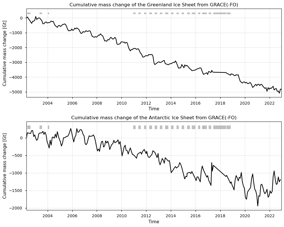
Figure 1. Greenland (top) and Antarctic (bottom) ice mass changes from GRACE(-FO), where shaded intervals depict data gaps longer than 1 month. Note the different range of the y-axis.
The provided graphs show the cumulative mass change of the Greenland Ice Sheet and the Antarctic Ice Sheet since 2002, as measured by GRACE(-FO) satellites. The GrIS shows a clear and consistent decline in mass, having lost approximately 5000 gigatonnes (Gt) over the period. The AIS mass change graph displays more pronounced fluctuations. For Greenland, mass loss is dominated by meltwater runoff, combined with the solid ice discharge towards the ocean across the grounding line of outlet glaciers. For Antarctica, mass loss primarily occurs through the discharge of ice across the grounding line, with surface melting playing a minor role. Here, interactions between the ice sheet and the warming ocean, combined with dynamic responses within the ice sheet itself (e.g. an acceleration of outlet glaciers due to a reduced buttressing from the ice shelves), are central to understanding why Antarctica’s mass is currently decreasing [1, 2, 3].
2.2 Spatio-temporal resolution and coverage of the GRACE(-FO) mass change estimates#
Now that we have visualized the temporal patterns of the mass changes, we can investigate the spatio-temporal resolution and extent of the GrIS and AIS mass changes. Let us begin by zooming in more on the temporal data gaps (coverage) and the temporal resolution in the time series:
Show code cell source
# Get time gaps
time_gap_months = 12 * ds["time"].diff("time").astype(int) / year_to_ns

# Create the plot
fig, ax = plt.subplots()
time_gap_months.plot(ax=ax, color='b')
ax.set_ylabel("Time gap [month]")
ax.grid(color='#95a5a6', linestyle='-', alpha=0.25)
ax.set_xlim(np.min(ds["time"]), np.max(ds["time"]))
ax.set_title("Time gap since last valid GRACE(-FO) measurement")
plt.show()
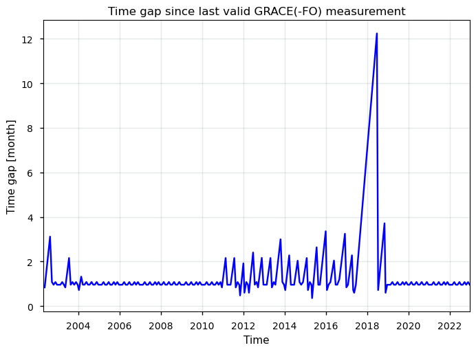
Figure 2. Time period between two consecutive GRACE(-FO) monthly solutions in the ice sheet GMB dataset.
The plot displays the time gaps in the GRACE(-FO) data collection over time, which are the same for the GrIS and the AIS, highlighting periods of consistent monthly data acquisition and (significant) data gaps. Generally, a temporal resolution of approximately 1 month (which is mostly the case) is observed, aligning with the optimal requirement proposed by GCOS [5]. More gaps in GRACE data, however, arise after 2011, which are due to sensor degradation. The most prominent feature is the large time gap around 2017-2018, where the gap extends up to 12 months. This significant gap corresponds to the end of the original GRACE mission and the transition period before the launch of the GRACE Follow-On (GRACE-FO) mission. During this period, there was an inability to acquire data, as the original GRACE satellites were decommissioned and the new GRACE-FO satellites were not yet operational. Because there is no systematic bias between the GRACE and GRACE-FO time series [4], this does not impact the overall trend and magnitude of the time series after 2018. In fact, for linear trend estimation, the presence of gaps (even long ones) scattered over the entire time series are almost irrelevant, as mass changes occurring during these gaps are still included in the subsequent solution. Long-term trend stability is therefore a major advantage of GMB data, as compared to the altimetry and input-output methods for ice mass change estimations.
Let us have the amount of gaps quantified to get an idea of the temporal data availability:
Show code cell source
start, end = ds["time"].isel(time=[0, -1]).dt.strftime("%d/%m/%Y").values.tolist()

for string, date in zip(("start", "end"), (start, end)):
    print(f"The {string:^5} date of the time series is", date)

expected = len(pd.date_range(start, end, freq="ME", inclusive="both"))
actual = len(set(ds["time"].dt.strftime("%Y%m").values))
for string, date in zip(("expected", "present"), (expected, actual)):
    print(f"The amount of months with mass change measurements that is {string} between these two dates is", date)

missing = 100 * abs(expected - actual) / expected
print(f"For a consistent monthly temporal resolution, the amount of months with missing data is {missing:.2f}%.")
The start date of the time series is 16/04/2002
The  end  date of the time series is 17/12/2022
The amount of months with mass change measurements that is expected between these two dates is 248
The amount of months with mass change measurements that is present between these two dates is 213
For a consistent monthly temporal resolution, the amount of months with missing data is 14.11%.
Concerning spatial coverage, a significant challenge in analyzing the ice sheet’s mass changes (especially for the GrIS) is deciding whether to include the peripheral glaciers and ice caps. The GRACE(-FO) GMB data include all ice masses in Greenland (and Antarctica), due to the coarse spatial resolution of several hundred kilometers during the data acquisition, which prevents differentiation between closely situated ice bodies. As a result, the mass changes of Greenland’s peripheral glaciers and ice caps, which contribute approximately 30-35 Gt/year [6], are included in these measurements. To exclude these peripheral areas from the GRACE(-FO) time series, a scaling factor of 0.84 is often used for the GrIS [7]. It must be furthermore noted that only mass changes of ice above buoyancy are considered in the GMB dataset (of which the impact is, however, relatively limited for the GrIS but can be significant for the AIS, due to the presence of more floating ice and ice grounded below present-day sea level).
The lack of downloadable gridded data further complicates the spatial resolution issue (in fact, since there are no gridded data, the term “spatial resolution” is not applicable for this C3S dataset), although such pixel-by-pixel data are available from other sources like the TU Dresden website. The currently available data are provided as time series for the entire ice sheet’s and their basins, which is too coarse to meet GCOS requirements and poses challenges, for example for ice sheet models that require gridded inputs.
3. Ice sheet mass change trends and sea level contribution over time#
3.1 Linear and quadratic ice sheet-wide mass change trends#
With the imformation above, let us now go on and calculate linear and quadratic trends for the ice sheet mass change product:
Show code cell source
fig, axs = plt.subplots(len(variables), 1, layout="constrained")
colors = {
    "data": "black",
    "linear": "blue",
    "quadratic": "red"
}
for ax, da in zip(axs, ds.data_vars.values()):
    da = da.dropna("time")
    print(da.attrs["region"] + ":")
    for label, degree, color in zip(
        (
            "Linear",
            "Quadratic",
        ),
        (1, 2),
        (colors["linear"], colors["quadratic"]),
    ):
        # Compute coefficients
        coeffs = da.polyfit("time", degree)["polyfit_coefficients"]

        # Plot trends and print stats
        equation = []
        for deg, coeff in coeffs.groupby("degree"):
            coeff = coeff.squeeze() * (year_to_ns**deg)
            if deg == degree:
                if deg == 1:
                    quantity = "slope"
                    units = "Gt/yr"
                elif deg == 2:
                    quantity = "acceleration"
                    units = "Gt/yr^2"
                else:
                    raise ValueError(f"{deg=}")
                print(
                    f"\tThe {quantity} of the ice sheet mass change is {degree*coeff:.3f} {units}."
                )
                if deg == 1:
                    _, p_value = scipy.stats.kendalltau(da["time"], da)
                    significance_level = 0.05
                    is_significant = p_value < significance_level
                    print(
                        " ".join(
                            [
                                "\tThe trend",
                                "is significant"
                                if is_significant
                                else "is not significant",
                                f"at an alpha level of {significance_level}, i.e. a monotonic trend",
                                "is present." if is_significant else "is not present.",
                            ]
                        )
                    )
            equation.append(
                f"{float(coeff):+.3f}{'x' if deg else ''}{f'$^{deg}$' if deg>1 else ''}"
            )
        label = f"{label}: {' '.join(equation[::-1])}"
        fit = xr.polyval(da["time"], coeffs)
        fit.plot(label=label, ax=ax, color=color)
    da.plot(label="Ice sheet mass change data", ax=ax, color='k')
    ax.set_title(f"{da.attrs['region']}")
    ax.set_xlim(np.min(ds["time"]), np.max(ds["time"]))
    ax.grid(color='#95a5a6', linestyle='-', alpha=0.25)
    ax.legend()
Cumulative mass change of the Greenland Ice Sheet from GRACE(-FO):
	The slope of the ice sheet mass change is -251.329 Gt/yr.
	The trend is significant at an alpha level of 0.05, i.e. a monotonic trend is present.
	The acceleration of the ice sheet mass change is 3.240 Gt/yr^2.
Cumulative mass change of the Antarctic Ice Sheet from GRACE(-FO):
	The slope of the ice sheet mass change is -89.873 Gt/yr.
	The trend is significant at an alpha level of 0.05, i.e. a monotonic trend is present.
	The acceleration of the ice sheet mass change is -2.354 Gt/yr^2.
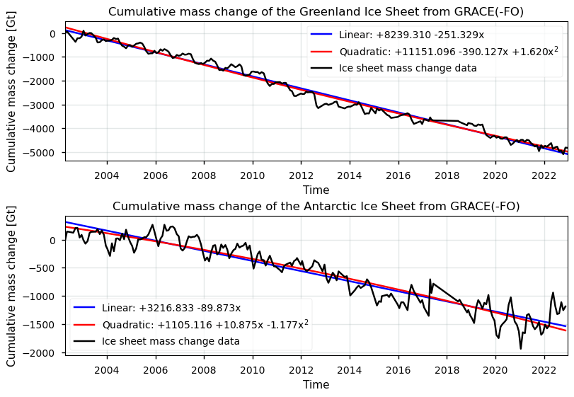
Figure 3. Linear and quadratic trends of ice sheet mass changes for the (above) GrIS and (below) AIS from the ice sheet GMB dataset.
The GRACE(-FO) data plots illustrate the cumulative mass changes of the Greenland and Antarctic Ice Sheets over time. Both the Greenland and Antarctic Ice Sheets exhibit significant ongoing mass loss, with the statistical significance of the trends underscoring the robustness of these findings. The linear and quadratic trend lines, depicted in red and green respectively, provide a clear visual representation of these trends, highlighting the critical changes occurring in the polar regions.
3.2 Quantifying ice sheet-related global sea level contributions#
We furthermore note again that GRACE(-FO) cannot detect changes in floating ice and ice below buoyancy for ice grounded below sea level. Mass change processes occurring beyond the grounding line, such as a retreating calving front, ocean-induced melt beneath the ice shelves, as well as changes to the part of the ice that is grounded below sea level (or in other words ice below buouyancy) will therefore not be detectable because it is occupied by the same mass of water. In that regard, GMB measurements by GRACE(-FO) are immediately convertible to sea level contributions. For the contributions of ice sheets, we assume that 361.8 Gt of ice will raise global sea levels by 1 mm [e.g. 11] (where 361.8 Gt of ice is equivalent to 394.67 km\(^3\) ice):
\( h_{SLE} \) [mm] \( = -\dfrac{M_{GRACE}}{361.8} \)
where \(M_{GRACE}\) is the cumulative mass change of the ice sheets measured by GRACE(-FO) in Gt. Let us plot this:
Show code cell source
fig, axs = plt.subplots(len(variables), 1, layout="constrained")
colors = {
    "data": "black",
    "linear": "blue",
    "quadratic": "red"
}
# Convert mass change to global sea level change
ds_SL = -(ds/361.8)
for i, (var, da) in enumerate(ds_SL.data_vars.items()):
    if i == 0:
        da.attrs["region"] = "Cumulative global sea level contribution of the Greenland Ice Sheet from GRACE(-FO)"

    elif i == 1:
        da.attrs["region"] = "Cumulative global sea level contribution of the Antarctic Ice Sheet from GRACE(-FO)"
    else:
        da.attrs["region"] = da.attrs["long_name"].split("_", 1)[0].title()
    da.attrs["long_name"] = "Sea level contribution (mm)"
# Plot the data and trends
for ax, da in zip(axs, ds_SL.data_vars.values()):
    da = da.dropna("time")
    print(da.attrs["region"] + ":")
    for label, degree, color in zip(
        (
            "Linear",
            "Quadratic",
        ),
        (1, 2),
        (colors["linear"], colors["quadratic"]),
    ):
        # Compute coefficients
        coeffs = da.polyfit("time", degree)["polyfit_coefficients"]

        # Plot trends and print stats
        equation = []
        for deg, coeff in coeffs.groupby("degree"):
            coeff = coeff.squeeze() * (year_to_ns**deg)
            if deg == degree:
                if deg == 1:
                    quantity = "slope"
                    units = "mm/yr"
                elif deg == 2:
                    quantity = "acceleration"
                    units = "mm/yr^2"
                else:
                    raise ValueError(f"{deg=}")
                print(
                    f"\tThe {quantity} of the global sea level contribution is {degree*coeff:.3f} {units}."
                )
                if deg == 1:
                    _, p_value = scipy.stats.kendalltau(da["time"], da)
                    significance_level = 0.05
                    is_significant = p_value < significance_level
                    print(
                        " ".join(
                            [
                                "\tThe trend",
                                "is significant"
                                if is_significant
                                else "is not significant",
                                f"at an alpha level of {significance_level}, i.e. a monotonic trend",
                                "is present." if is_significant else "is not present.",
                            ]
                        )
                    )
            equation.append(
                f"{float(coeff):+.3f}{'x' if deg else ''}{f'$^{deg}$' if deg>1 else ''}"
            )
        label = f"{label}: {' '.join(equation[::-1])}"
        fit = xr.polyval(da["time"], coeffs)
        fit.plot(label=label, ax=ax, color=color)
    da.plot(label="Ice sheet mass change data", ax=ax, color='k')
    ax.set_title(f"{da.attrs['region']}")
    ax.set_xlim(np.min(ds_SL["time"]), np.max(ds_SL["time"]))
    ax.grid(color='#95a5a6', linestyle='-', alpha=0.25)
    ax.legend()
Cumulative global sea level contribution of the Greenland Ice Sheet from GRACE(-FO):
	The slope of the global sea level contribution is 0.695 mm/yr.
	The trend is significant at an alpha level of 0.05, i.e. a monotonic trend is present.
	The acceleration of the global sea level contribution is -0.009 mm/yr^2.
Cumulative global sea level contribution of the Antarctic Ice Sheet from GRACE(-FO):
	The slope of the global sea level contribution is 0.248 mm/yr.
	The trend is significant at an alpha level of 0.05, i.e. a monotonic trend is present.
	The acceleration of the global sea level contribution is 0.007 mm/yr^2.
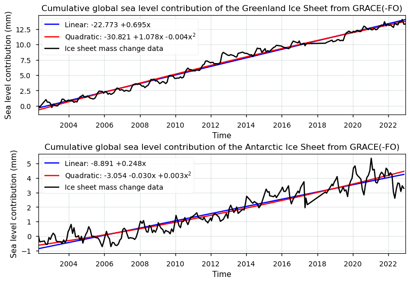
Figure 4. Contribution of ice sheet mass changes to global sea level for the (above) GrIS and (below) AIS from the ice sheet GMB dataset.
The linear trends and their significance show a consistent ongoing increase in sea level contributions, with Greenland contributing more significantly compared to Antarctica. The trends and their magnitudes observed in the GRACE(-FO) data for both the Greenland and Antarctic Ice Sheets are broadly consistent with the findings reported in the literature from other mass change estimation methods (e.g. [9, 12, 13]), highlighting the reliability and quality-richness of GRACE(-FO) data with respect to capturing significant ice mass changes and their impact on global sea level rise.
4. Short summary and take-home messages#
GRACE(-FO) data provide a valuable long-term dataset for detecting trends in ice sheet mass changes, making them a reliable indicator of climate change. With over 20 years of (mostly) continuous data, the dataset enables the assessment of long-term variations in ice sheet mass balance at the basin and ice sheet-wide scales. Unlike other remote sensing methods that infer mass changes indirectly, GRACE(-FO) directly measures gravitational anomalies, capturing mass redistribution patterns across both the GrIS and AIS. Although the IPCC standard for climate normals is 30 years, the dataset’s continuity from GRACE (2002–2017) to GRACE-FO (2018–present) ensures that clear temporal patterns can be identified, making it a crucial tool for climate and global water cycle studies.
However, GRACE(-FO) has limitations, including a coarse spatial resolution (several hundred kilometers), which restricts its ability to resolve small-scale variations and separate closely situated ice bodies (e.g. Greenland and its peripheral glaciers/ice caps, including the adjacent Canadian ice caps). Additional uncertainties arise mainly from complex processes such as signal leakage and geophysical corrections [10]. The dataset also lacks pixel-level (gridded) mass change and error estimates, limiting its applicability to grid-based assessments. Additionally, users should also acknowledge what GRACE(-FO) ice mass changes represent. GRACE(-FO) only considers patterns of mass redistribution by ice masses above buoyancy (i.e. solid ice discharge and changing rates of runoff/accumulation), meaning floating ice and ice grounded below sea level do not contribute to the measured mass change. For the GrIS, peripheral glaciers and ice caps are included, whereas for the Antarctic Ice Sheet AIS, ice shelves beyond the grounding line are excluded.
Despite occasional data gaps and relatively high uncertainty values in some measurements, GRACE(-FO) remains a powerful tool for quantifying the mean, variability, and trends in ice mass changes because (1) the amount of missing data is relatively limited and these data gaps do not impact the values of consecutive cumulative mass anomalies, (2) the temporal resolution is mostly consistent at 1-monthly spaced time intervals, (3) the number of consecutive years is generally sufficient to filter out inter and intrayearly variability, and (4) the presence of data gaps in the time series do not impact the overall trend and magntiude of the mass changes and sea level contributions (e.g. [4]). The dataset’s ability to directly convert ice mass changes into sea level contributions makes it a convenient tool for climate change monitoring and global water cycle assessments. Trends in ice sheet mass changes and sea level contributions from the C3S product furthermore agree well with general findings in the literature from other mass change estimation methods [8, 9, 12, 13], further adding credibility to the data. While certain limitations are thus present, its role as a direct measurement tool for ice sheet mass loss makes it essential for evaluating ice sheet stability and contributions to sea level rise.
ℹ️ If you want to know more#
Key resources#
“Gravimetric mass balance data for the Antarctic and Greenland ice sheets from 2003 to 2022 derived from satellite observations” on the CDS.
Documentation on the CDS and the ECMWF Confluence Wiki (Copernicus Knowledge Base).
The data portal with GMB data from the data provider (TU Dresden) for the GrIS and the AIS.
C3S EQC custom functions,
c3s_eqc_automatic_quality_controlprepared by B-Open.
References#
[1] Forsberg, R., Sørensen, L.S. and Simonsen, S.B. (2017). Greenland and Antarctica Ice Sheet Mass Changes and Effects on Global Sea Level. Surv. Geophys., 38, 89–104. https://doi.org/10.1007/s10712-016-9398-7
[2] Groh, A., Horwath, M., Horvath, A., Meister, R., Sørensen, L.S., Barletta, V.R., Forsberg, R., Wouters, B., Ditmar, P., Ran, J., Klees, R., Su, X., Shang, K., Guo, J., Shum, C.K., Schrama, E., and Shepherd, A. (2019). Evaluating GRACE Mass Change Time Series for the Antarctic and Greenland Ice Sheet, Geosciences, 9(10). https://doi.org/10.3390/geosciences9100415
[3] van den Broeke, M., Enderlin, E. M., Howat, I. M., Kuipers Munneke, P., Noël, B. P. Y., van de Berg, W. J., van Meijgaard, E., and Wouters, B. (2016). On the recent contribution of the Greenland ice sheet to sea level change, The Cryosphere, 10, 1933–1946, https://doi.org/10.5194/tc-10-1933-2016
[4] Velicogna, I., Mohajerani, Y., A, G., Landerer, F., Mouginot, J., Noel, B., Rignot, E., Sutterley, T., van den Broeke, M., van Wessem, M., and Wiese, D. (2020). Continuity of Ice Sheet Mass Loss in Greenland and Antarctica from the GRACE and GRACE Follow-On Missions. Geophys. Res. Lett. 47. https://doi.org/10.1029/2020GL087291
[5] GCOS (Global Climate Observing System) (2022). The 2022 GCOS ECVs Requirements (GCOS-245). World Meteorological Organization: Geneva, Switzerland. doi: https://library.wmo.int/idurl/4/58111
[6] Otosaka, I. N., Shepherd, A., Ivins, E. R., Schlegel, N.-J., Amory, C., van den Broeke, M. R., Horwath, M., Joughin, I., King, M. D., Krinner, G., Nowicki, S., Payne, A. J., Rignot, E., Scambos, T., Simon, K. M., Smith, B. E., Sørensen, L. S., Velicogna, I., Whitehouse, P. L., A, G., Agosta, C., Ahlstrøm, A. P., Blazquez, A., Colgan, W., Engdahl, M. E., Fettweis, X., Forsberg, R., Gallée, H., Gardner, A., Gilbert, L., Gourmelen, N., Groh, A., Gunter, B. C., Harig, C., Helm, V., Khan, S. A., Kittel, C., Konrad, H., Langen, P. L., Lecavalier, B. S., Liang, C.-C., Loomis, B. D., McMillan, M., Melini, D., Mernild, S. H., Mottram, R., Mouginot, J., Nilsson, J., Noël, B., Pattle, M. E., Peltier, W. R., Pie, N., Roca, M., Sasgen, I., Save, H. V., Seo, K.-W., Scheuchl, B., Schrama, E. J. O., Schröder, L., Simonsen, S. B., Slater, T., Spada, G., Sutterley, T. C., Vishwakarma, B. D., van Wessem, J. M., Wiese, D., van der Wal, W., and Wouters, B. (2023). Mass balance of the Greenland and Antarctic ice sheets from 1992 to 2020, Earth Syst. Sci. Data, 15, 1597–1616, https://doi.org/10.5194/essd-15-1597-2023
[7] Colgan, W., Abdalati, W., Citterio, M., Csatho, B., Fettweis, X., Luthcke, S., Moholdt, G., Simonsen, S.B., and Stober, M. (2015). Hybrid glacier Inventory, Gravimetry and Altimetry (HIGA) mass balance product for Greenland and the Canadian Arctic. Remote Sensing of Environment, 168, 24–39. https://doi.org/10.1016/j.rse.2015.06.016
[8] Fox-Kemper, B., H.T. Hewitt, C. Xiao, G. Aðalgeirsdóttir, S.S. Drijfhout, T.L. Edwards, N.R. Golledge, M. Hemer, R.E. Kopp, G. Krinner, A. Mix, D. Notz, S. Nowicki, I.S. Nurhati, L. Ruiz, J.-B. Sallée, A.B.A. Slangen, and Y. Yu (2021). Ocean, Cryosphere and Sea Level Change. In Climate Change 2021: The Physical Science Basis. Contribution of Working Group I to the Sixth Assessment Report of the Intergovernmental Panel on Climate Change [Masson-Delmotte, V., P. Zhai, A. Pirani, S.L. Connors, C. Péan, S. Berger, N. Caud, Y. Chen, L. Goldfarb, M.I. Gomis, M. Huang, K. Leitzell, E. Lonnoy, J.B.R. Matthews, T.K. Maycock, T. Waterfield, O. Yelekçi, R. Yu, and B. Zhou (eds.)]. Cambridge University Press, Cambridge, United Kingdom and New York, NY, USA, pp. 1211–1362, https://doi.org/110.1017/9781009157896.011
[9] Bamber, J. L., Westaway, R. M., Marzeion, B., and Wouters, B. (2018). The land ice contribution to sea level during the satellite era. Environ. Res. Lett. 13, https://doi.org/10.1088/1748-9326/aac2f0
[10] Barletta, V. R., Sørensen, L. S., and Forsberg, R. (2013). Scatter of mass changes estimates at basin scale for Greenland and Antarctica, The Cryosphere, 7, 1411–1432, https://doi.org/10.5194/tc-7-1411-2013
[11] Ludwigsen, C.B., Andersen, O.B., Marzeion, B., Malles, J.H., Müller Schmied, H., Döll, P., Watson, C., and King, M.A. (2024). Global and regional ocean mass budget closure since 2003. Nat. Commun. 15, 1416 (2024). https://doi.org/10.1038/s41467-024-45726-w
[12] The IMBIE Team (2019). Mass balance of the Greenland Ice Sheet from 1992 to 2018. Nature, 579, 233–239. https://doi.org/10.1038/s41586-019-1855-2
[13] The IMBIE Team (2018). Mass balance of the Antarctic Ice Sheet from 1992 to 2017. Nature 558, 219–222. https://doi.org/10.1038/s41586-018-0179-y