

1.3.1. Comparing sea ice concentration products to the sea ice edge product#
Production date: 14-04-2025
Produced by: Timothy Williams, Nansen Environment and Remote Sensing Center
🌍 Use case: Assessing the uncertainty of sea ice concentration products#
❓ Quality assessment question#
How do the sea ice concentration products compare to the sea ice edge product?
📢 Quality assessment statement#
These are the key outcomes of this assessment
We find that both sea ice concentration products generally produce a lower ice extent than the ice edge product, but that the bias and IIEE (Integrated Ice Edge Error) are lower for the SSMIS (Special Sensor Microwave Imager/Sounder) products than the AMSR (Advanced Microwave Scanning Radiometer) product. This is consistent with the results from the notebook on the assessment of climate change on the satellite sea ice concentration products, which showed that the SSMIS product had a higher extent than the AMSR. Comparing the Arctic and the Antarctic, the signs of the metrics are the same but the sizes of the discrepancies are larger in Antarctica. The differences between these products give one estimate of the uncertainty in the sea ice concentration products and the extents derived from them.
📋 Methodology#
We first take the sea ice concentration dataset, which has two CDR (Climate Data Record) products from EUMETSAT (European Organisation for the Exploitation of Meteorological Satellites) OSI SAF (Ocean and Sea Ice Satellite Application Facility):
SSMIS (1979-2020)
AMSR (2003-2017)
Then we compare it to the sea ice edge and type dataset, and use the product:
Sea ice edge CDR (1978-2020)
To compare the two products we first convert the sea ice concentration (SIC) to an ice/water classification according to the criteria used to create the ice edge product which is SIC > 30%. We then compare the classification from each SIC product to the classification from the sea ice edge product, which is determined by considering all passive microwave SIC products available (including others not in the CADS). The comparison is done by calculating areas \(A_{\rm over}\) (area of the grid cells with ice in the SIC product but no ice in the ice edge product) and \(A_{\rm under}\) (area of the grid cells with no ice in the SIC product but ice in the ice edge product). The final metrics used are the “bias”, defined as \(A_{\rm over} - A_{\rm under}\), and the IIEE (integrated ice edge error, or the total area where the classification from the SIC product disagrees with the sea ice edge product), defined as \(A_{\rm over} + A_{\rm under}\).
The “Analysis and results” section is structured as follows:
📈 Analysis and results#
1. Parameters, requests and functions definition#
Define parameters and formulate requests for downloading with the EQC toolbox.
Define functions to be applied to process and reduce the size of the downloaded data.
Define functions to post-process and visualize the data.
1.1 Import libraries#
Import the required libraries, including the EQC toolbox.
1.2 Set parameters#
Set the time period to cover with start_year and stop_year.
Also specify regrid_kwargs, which are options to use for interpolating the sea ice concentration product to the grid used for the sea ice edge product.
1.3 Define requests#
Define the requests for downloading the sea ice concentration data using the EQC toolbox.
1.4 Functions for creating the time series of differences between the datasets#
add_boundsis a small function to add longitude and latitude bounds if we are using conservative interpolation.interpolate_to_siedge_gridinterpolates a sea ice concentration dataset to the sea ice edge grid.get_interpolated_datais a wrapper function which modifies some dimensions and attributes and callsinterpolate_to_siedge_gridif requested.get_siedge_dataloads the sea ice edge data. It is also transformed withget_interpolated_databut without interpolation since the concentration data is being transformed onto its grid.compare_siconc_vs_siedgecalculates the metrics measuring the differences between the sea ice concentration dataset and the sea ice edge one.compute_siconc_siedge_time_seriesis the function that is called byc3s_eqc_automatic_quality_control.download.download_and_transform. It callsget_siedge_data,get_interpolated_data, and creates the final time series withcompare_siconc_vs_siedge.
1.5 Postprocessing and plotting functions#
rearrange_year_vs_dayofyearchanges the dataset from having a single time dimension to having two: the year and the Julian day of the year.make_subplotmakes one plot of a variable with a different line for each year (shown with a legend if there are not too many lines; otherwise it is shown with a colorbar), and with the \(x\) axis being the Julian day of the year.plot_against_dayofyearcallsmake_subplotfor each of the extent bias and the integrated ice edge error (IIEE).
2. Download and transform#
This is where the data is downloaded, transformed with compute_siconc_siedge_time_series, and saved to disk by the EQC toolbox. If the code is rerun the transformed data is loaded from the disk.
It is then post-processed with rearrange_year_vs_dayofyear to be used by plot_against_dayofyear.
3. Results#
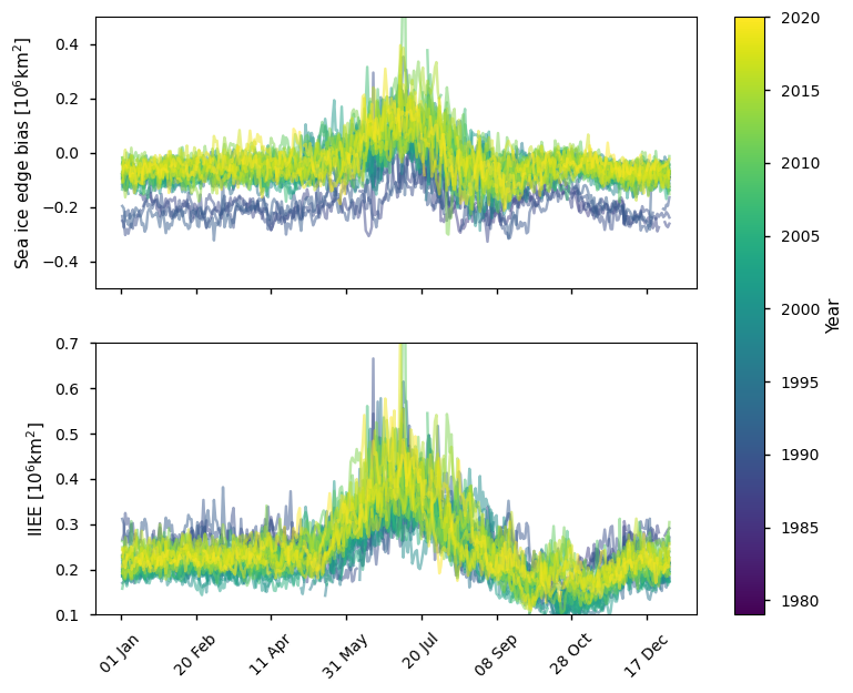
3.1 Arctic sea ice edge#
Below we plot the difference in ice edge for the Arctic between the ice edge product and the ice mask (sea ice concentration >30%) derived from the SSMIS sea ice concentration CDR, which covers the period 1979 - 2015. In winter this product has a negative bias compared to the ice edge product (between 0 - 0.2 million km\(^2\)), while in summer it has a positive bias (between 0 - 0.4 million km\(^2\)). The IIEE is generally between 0.2 - 0.3 million km\(^2\) in late winter, being between 0.1 - 0.3 million km\(^2\) earlier in winter with a minimum around October. The IIEE is highest in summer (between 0.3 - 0.6 million km\(^2\)).
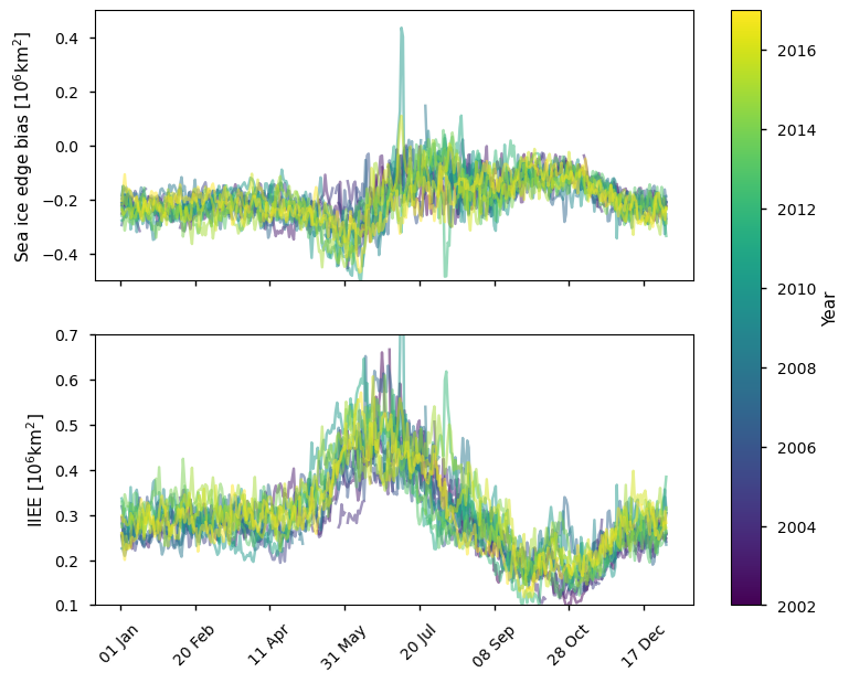
Below we plot the difference in ice edge for the Arctic between the ice edge product and the ice mask (sea ice concentration >30%) derived from the AMSR sea ice concentration CDR, which covers the period 2002 - 2017. This product has a consistent negative bias compared to the ice edge product (between 0 - 0.4 million km\(^2\)). In late winter (January - April) it is nearly constant around -0.2 million km\(^2\), but it is more variable at other times of the year. The IIEE is generally between 0.25 - 0.35 million km\(^2\) in late winter, being between 0.15 - 0.35 million km\(^2\) earlier in winter with a minimum around October. The IIEE is highest in summer (between 0.3 - 0.6 million km\(^2\)).
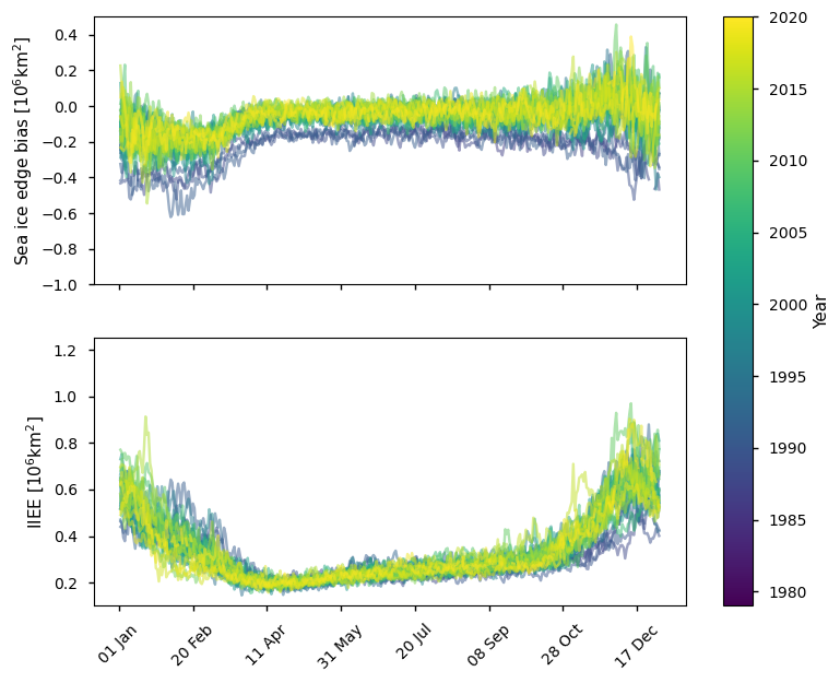
3.2 Antarctic sea ice edge#
Below we plot the difference in ice edge for the Antarctic between the ice edge product and the ice mask (sea ice concentration >30%) derived from the SSMIS sea ice concentration CDR, which covers the period 1979 - 2015. It is biased lower than the ice edge product by an amount between 0 and 0.5 million km\(^2\), with the difference (and the spread of differences) being greatest in the summer. The IIEE is also greater in summer (between 0.4 - 0.9 million km\(^2\)), while it is between 0.2 - 0.4 million km\(^2\) in winter. The IIEE also has more spread in summer than in winter.
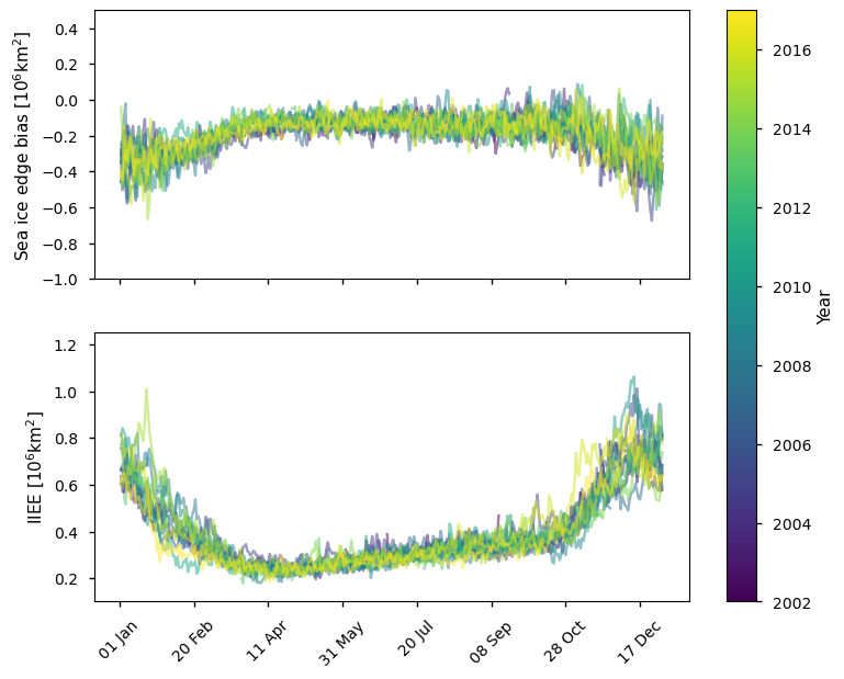
Below we plot the difference in ice edge for the Antarctic between the ice edge product and the ice mask (sea ice concentration >30%) derived from the AMSR sea ice concentration CDR, which covers the period 2002-2017. It is biased lower than the ice edge product by an amount between 0.25 and 0.75 million km\(^2\), with the difference (and the spread of differences) being greatest in the summer. The IIEE is also greater in summer (between 0.6 - 1.1 million km\(^2\)), while it is between 0.2 - 0.5 million km\(^2\) in winter. The IIEE also has more spread in summer than in winter.
ℹ️ If you want to know more#
Key resources#
Introductory sea ice materials:
Code libraries used:
C3S EQC custom functions,
c3s_eqc_automatic_quality_control, prepared by B-Open
References#
Ivanova, N., Pedersen, L. T., Tonboe, R. T., Kern, S., Heygster, G., Lavergne, T., Sørensen, A., Saldo, R., Dybkjær, G., Brucker, L., & Shokr, M. (2015). Inter-comparison and evaluation of sea ice algorithms: towards further identification of challenges and optimal approach using passive microwave observations. The Cryosphere, 9(5), 1797-1817, https://doi.org/10.5194/tc-9-1797-2015 .
Comiso, J. C., Cavalieri, D. J., Parkinson, C. L., & Gloersen, P. (1997). Passive microwave algorithms for sea ice concentration: A comparison of two techniques. Remote sensing of Environment, 60(3), 357-384, https://doi.org/10.1016/S0034-4257%2896%2900220-9 .
Buckley, E. M., Horvat, C., & Yoosiri, P. (2024). Sea Ice Concentration Estimates from ICESat-2 Linear Ice Fraction. Part 1: Multi-sensor Comparison of Sea Ice Concentration Products. EGUsphere, 2024, 1-19, https://doi.org/10.5194/egusphere-2024-3861 .