Biases in temperature trends at different pressure levels using CMIP6 across latitudinal bands

5.1.1. Biases in temperature trends at different pressure levels using CMIP6 across latitudinal bands#

Production date: 27-06-2025

Produced by: CMCC foundation - Euro-Mediterranean Center on Climate Change. Albert Martinez Boti and Lorenzo Sangelantoni.

🌍 Use case: Pressure-levels dependencies of temperature trends biases: informing model developers and model output users#

❓ Quality assessment question#

How is warming propagating across pressure levels and different latitudinal bands?
Is there signal consistence between CMIP6 ensemble results and ERA5, and among CMIP6 ensemble GCMs?

The vertical profile of temperature trends is widely recognised as an important fingerprint of climate change (e.g., [1],[2]),[3]. One of the most studied features of this vertical structure is the amplified warming in the tropical upper troposphere compared to the surface, commonly referred to as tropical tropospheric amplification [4]. This behaviour is consistent with the basic theory of moist adiabatic processes, which predicts stronger warming in the tropical free troposphere than near the surface due to latent heat release during deep convection [5].

While tropical amplification has been widely studied, other regions and their representation in CMIP6 models remain less explored. To develop a more comprehensive evaluation framework, it is essential to assess how warming propagates vertically across pressure levels and latitudinal bands. Understanding the vertical structure of temperature trends across these bands provides critical insights into model performance and the physical processes driving climate change. This vertical perspective is key for model developers to identify and diagnose persistent biases, such as errors in atmospheric circulation, lapse rates, and vertical energy transport, and thereby improve model simulations.

This assessment evaluates temperature mean and trend biases across multiple pressure levels using the full ensemble of CMIP6 models available through the Copernicus Climate Data Store (CDS). Model outputs are compared against the ERA5 reanalysis, which is used as the reference product. The analysis is performed over latitudinal bands—including Global, Northern and Southern hemispheres, Tropics, Extratropics, and Polar regions—to characterise spatial variability in biases and explore their dependence on latitude and atmospheric dynamics.

📢 Quality assessment statement#

These are the key outcomes of this assessment

Model spread in mean temperature climatology increases with altitude, especially above the tropopause, highlighting substantial uncertainty in simulating its height and structure—critical for model evaluation and development.
The median of CMIP6 climatological temperatures shows predominantly cold biases across all latitudinal bands, largest near 250–200 hPa. Near-surface and lower-stratosphere biases are smaller (though the spread is high), except in polar regions, where both the bias and the spread increase.
Temperature trends show robust tropospheric warming and stratospheric cooling across all latitudinal bands in both ERA5 and CMIP6. CMIP6 generally exhibits stronger warming trends than ERA5.
Tropical amplification of trends is evident, with trend magnitudes stronger in CMIP6 than in ERA5 (not necessarily the amplification). Amplification is also high when considering the southern-hemisphere for both ERA5 and CMIP6.
Trend magnitudes and structures vary with dataset processing, leading to moderate to low confidence in tropospheric warming rates (IPCC AR5 [6]).
ERA5 is used as the reference dataset to reduce inhomogeneities, though the use of multiple datasets is recommended to capture reference products uncertainties (as in [7])

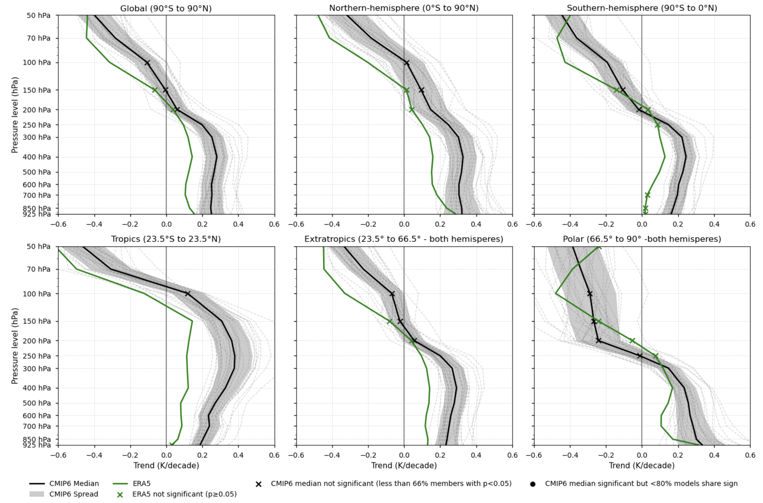
Visual abstract — Fig. 5.1.1.1 Vertical profiles of the annual mean temperature trend (1979-2014). Each subplot corresponds to a latitudinal band (Global, Northern Hemisphere, Southern Hemisphere, Tropics, Extratropics, and Polar). ERA5 is shown as a green line, the CMIP6 ensemble median as a solid black line, individual CMIP6 models as grey dashed lines, and the ensemble spread as a grey shaded area. ERA5 points with non-significant trends (p-value > 0.05) are marked with green crosses. For the CMIP6 ensemble median, trend significance is assessed using agreement categories based on the approach described in the IPCC AR6 Atlas (pp. 1945–1950). Black crosses indicate pressure levels where fewer than 66% of models show statistically significant trends (p-value < 0.05). If over 66% of the models are significant but fewer than 80% agree on the sign of the trend, a black dot is placed on the CMIP6 ensemble median to indicate low directional agreement.#

📋 Methodology#

A subset of 33 models from CMIP6 are used to assess temperature trends and climatology at different pressure levels, comparing them with those derived from the ERA5 reference product. The analysis is performed across the following latitudinal bands:

Global (90°S to 90°N)
Northern-hemisphere (0°S to 90°N)
Southern-hemisphere (90°S to 0°N)
Tropics (23.5°S to 23.5°N)
Extratropics (23.5° to 66.5° in both hemispheres)
Polar (66.5° to 90° in both hemispheres)

For each latitudinal band, temperature climatology and trends are calculated at the following pressure levels: 925, 850, 700, 600, 500, 400, 300, 250, 200, 150, 100, 70, and 50 hPa. Results are presented using subplots—one per band—showing the vertical profiles of climatology and trends for each CMIP6 model alongside ERA5, following an approach similar to [7], who analysed ground- and satellite-based temperature trends over 1979–2018. Biases in both climatology and trends are also shown. The analysis period is 1979–2014.

The analysis and results follow the next outline:

1. Parameters, requests and functions definition

1.1. Import packages
1.2. Define Parameters
1.3. Define models
1.4. Define ERA5 request
1.5. Define model requests
1.6. Functions to cache

2. Downloading and processing

2.1. Download and transform ERA5
2.2. Download and transform models

3. Plot and describe results

3.1. Define plotting functions
3.2. Plot climatology maps
3.3. Plot mean bias maps
3.4. Plot trend maps
3.5. Plot trend bias maps
3.6. Results summary and discussion - Climatologies
3.7. Results summary and discussion - Trends

📈 Analysis and results#

1. Parameters, requests and functions definition#

1.1. Import packages#

1.2. Define Parameters#

In the “Define Parameters” section, various customisable options for the notebook are specified:

The start and end years of the historical period can be adjusted using the parameters year_start and year_stop. The default period (1979–2014) is selected to ensure consistency with the satellite era in ERA5, which began assimilating satellite observations in 1979.
The chunk selection allows the user to define if dividing into chunks when downloading the data on their local machine. Although it does not significantly affect the analysis, it is recommended to keep the default value for optimal performance.
variable and collection_id are not customisable for this assessment and are set to ‘temperature’ and ‘CMIP6’. Expert users can use this notebook as a guide to create similar analyses for other variables or model sets (such as CORDEX).

1.3. Define models#

The following climate analyses are performed considering the CMIP6 models that have available both the historical and SSP5-8.5 experiments within the Climate Data Store (CDS).

1.4. Define ERA5 request#

Within this notebook, ERA5 serves as the reference product. In this section, we set the required parameters for the cds-api data-request of ERA5.

request_era_ps_mask is used to retrieve surface pressure data used to identify and mask out pressure levels below the surface.

1.5. Define model requests#

In this section we set the required parameters for the cds-api data-request.

1.6. Functions to cache#

In this section, functions that will be executed in the caching phase are defined. Caching is the process of storing copies of files in a temporary storage location, so that they can be accessed more quickly. This process also checks if the user has already downloaded a file, avoiding redundant downloads.

Description of the main functions:

compute_band_trends_clim: Computes vertical profiles of temperature climatology and trends. It first calculates annual means, then calls get_latband_mean, which averages over longitudes for each latitude within the band, and subsequently across those latitudes. The resulting time series is passed to compute_trends_clim to estimate the climatology and linear trend.
compute_trends_clim: Computes the climatology and linear trend of a time series using ordinary least squares regression.

Show code cell source Hide code cell source

def get_latband_mean(ds, lat_min=None, lat_max=None):
    lat_start = ds.latitude.sel(latitude=lat_max, method="nearest")
    lat_end = ds.latitude.sel(latitude=lat_min, method="nearest")
    
    # Ensure correct slicing order for descending or ascending latitude
    lat_slice = slice(min(lat_start.item(), lat_end.item()), max(lat_start.item(), lat_end.item()))
    ds=ds.sel(latitude=lat_slice)
    ds=ds.mean(dim="longitude", skipna=True)
    return ds.mean(dim="latitude", skipna=True)

def get_symmetric_latband_mean(ds, lat_min=None, lat_max=None):
    north = get_latband_mean(ds, lat_min=lat_min, lat_max=lat_max)
    south = get_latband_mean(ds, lat_min=-lat_max, lat_max=-lat_min)
    return xr.concat([north, south], dim="dummy").mean(dim="dummy", skipna=True)

def round_plev(ds, decimals=2):
    if 'plev' in ds.coords:
        rounded_plev = ds['plev'].round(decimals=decimals)
        ds = ds.assign_coords(plev=("plev", rounded_plev.data))
    return ds


def compute_trends_clim(ds,obs=False):
    def linregress_ufunc(y, x):
        slope, intercept, r_value, p_value, std_err = linregress(x, y)
        return slope, p_value

    da = list(ds.data_vars.values())[0]
    da_clim= da.mean(dim="time")
    time = da['time'].values.astype('float64')  
    slope, pval = xr.apply_ufunc(
        linregress_ufunc,
        da,  # shape: (pressure_level, band, time)
        time,
        input_core_dims=[['time'], ['time']],
        output_core_dims=[[], []],
        vectorize=True,
        dask='parallelized',
        output_dtypes=[float, float]
    )
    ds = xr.Dataset(
        {
            "clim":da_clim,
            "slope": slope,
            "p":pval,
        }
    )

    # harmonize pressure coordinate name
    if obs==False:
        ds = ds.rename({"plev": "pressure_level"})
    
    ds['signif'] = (ds['p'] < 0.05).astype(int)
    
    return ds


def compute_band_trends_clim(
    ds, year_start, year_stop, obs=False,
):
    if obs==True:
        ds_ps_mask = download.download_and_transform(
            *request_era_ps_mask,
            chunks=chunks,
        )
        masked_list = []
        ds = ds.assign_coords(pressure_level=("pressure_level", ds.pressure_level.values * 100))

        for level in ds.pressure_level.values:
            mask = ds_ps_mask['sp'] >= level
            mask = mask.expand_dims(pressure_level=[level])
            masked_list.append(mask)

        # Concatenate along pressure_level
        mask_levels = xr.concat(masked_list, dim='pressure_level')
        ds = ds.where(mask_levels)
        ds = ds.sortby("latitude")

    ds = ds.convert_calendar('proleptic_gregorian', align_on='date', use_cftime=False)
    if 'areacella' in ds:
        ds = ds.drop_vars('areacella')
    # Compute means for each band
    latband_mean_global = get_latband_mean(ds, lat_min=-90, lat_max=90)
    latband_mean_NH = get_latband_mean(ds, lat_min=0, lat_max=90)
    latband_mean_SH = get_latband_mean(ds, lat_min=-90, lat_max=0)
    latband_mean_tropics = get_latband_mean(ds, lat_min=-23.5, lat_max=23.5)
    latband_mean_extratropics = get_symmetric_latband_mean(ds, lat_min=23.5, lat_max=66.5)
    latband_mean_polar = get_symmetric_latband_mean(ds, lat_min=66.5, lat_max=90)

    # Add a new coordinate for each band and concatenate
    ds = xr.concat(
        [latband_mean_global, latband_mean_NH, latband_mean_SH,latband_mean_tropics, latband_mean_extratropics, latband_mean_polar],
        dim=xr.DataArray(["Global","Northern-hemisphere", "Southern-hemisphere",
                          "Tropics", "Extratropics", "Polar"], dims="band", name="band")
    )
    ds=ds.resample(time="YS").mean()
    ds = round_plev(ds, decimals=0)
    ds = ds.chunk({"time": -1}).compute()  # single chunk over time
    ds=compute_trends_clim(ds,obs=obs)
    return ds

2. Downloading and processing#

2.1. Download and transform ERA5#

In this section, the download.download_and_transform function from the ‘c3s_eqc_automatic_quality_control’ package is used to retrieve ERA5 monthly reference data, compute annual means, calculate latitudinal band averages, and derive the climatology and linear trend at each pressure level for each latitudinal band. Results are cached to avoid redundant downloads and repeated processing.

2.2. Download and transform models#

In this section, the download.download_and_transform function from the ‘c3s_eqc_automatic_quality_control’ package is employed to download monthly data from the CMIP6 models, compute annual means, calculate latitudinal band averages, and derive the climatology and linear trend at each pressure level for each latitudinal band. Results are cached to avoid redundant downloads and repeated processing.

model='access_cm2'
model='awi_cm_1_1_mr'
model='canesm5'
model='canesm5_canoe'
model='ciesm'
model='cmcc_cm2_sr5'
model='cesm2'
model='cmcc_esm2'
model='cnrm_cm6_1'
model='cnrm_cm6_1_hr'
model='cnrm_esm2_1'
model='ec_earth3_cc'
model='ec_earth3_veg_lr'
model='fgoals_g3'
model='fgoals_f3_l'
model='fio_esm_2_0'
model='gfdl_esm4'
model='hadgem3_gc31_ll'
model='hadgem3_gc31_mm'
model='iitm_esm'
model='inm_cm4_8'
model='inm_cm5_0'
model='ipsl_cm6a_lr'
model='kiost_esm'
model='miroc6'
model='miroc_es2l'
model='mcm_ua_1_0'
model='mpi_esm1_2_lr'
model='mri_esm2_0'
model='nesm3'
model='noresm2_mm'
model='taiesm1'
model='ukesm1_0_ll'

3. Plot and describe results#

This section will display the following results:

Vertical profiles of the climatology for each latitudinal band, including ERA5, the median of the CMIP6 models, and the model spread.
Vertical profiles of the mean bias for each latitudinal band, showing the median of the CMIP6 model biases and their spread.
Vertical profiles of the trend for each latitudinal band, including ERA5, the median of the CMIP6 models, and the spread.
Vertical profiles of the trend bias for each latitudinal band, showing the median of the CMIP6 model biases and their spread.

3.1. Define plotting functions#

The function plot_profile is used to display vertical profiles of the climatology and trend for each latitudinal band. When the bias option is set to False, ERA5 is shown as a green line, the CMIP6 ensemble median as a solid black line, individual CMIP6 models as grey dashed lines, and the model spread as a grey shaded area. When bias=True, the function instead plots the corresponding biases: the median CMIP6 bias is shown in blue, individual model biases in grey dashed lines, and their spread as a blue shaded area.

Show code cell source Hide code cell source

import matplotlib.pyplot as plt
import numpy as np
from collections import OrderedDict
from matplotlib.ticker import FixedLocator


def plot_profile(ds_era5, ds_models, plot_type='trend', yscale='log', bias=False):

    band_latlon = ("90°S to 90°N", "0°S to 90°N", "90°S to 0°N",
                   "23.5°S to 23.5°N", "23.5° to 66.5° - both hemisperes",
                   "66.5° to 90° -both hemisperes")    
    
    bands = ds_era5.band.values
    pressure = ds_era5.pressure_level.values

    # Convert pressure to hPa if needed
    if np.nanmax(pressure) > 2000:  # assume Pa -> convert to hPa
        pressure = pressure / 100.0

    # Sort pressure descending
    sort_idx = np.argsort(pressure)[::-1]
    pressure_desc = pressure[sort_idx]

    # Setup according to plot type
    if plot_type == 'trend':
        factor = 3.15576e17  # from K/ns to K/decade
        var_key = 'slope'
        nrows, ncols = 2, 3
    elif plot_type == 'mean':
        factor = -273.15  # Kelvin to Celsius
        var_key = 'clim'
        nrows, ncols = 3, 2
    else:
        raise ValueError("plot_type must be 'trend' or 'mean'")

    fig, axes = plt.subplots(nrows, ncols, figsize=(15, 10), sharey=True)
    axes = axes.flatten()

    for i, band_name in enumerate(bands):
        ax = axes[i]

        # Extract data
        if plot_type == 'trend':
            era5_vals = ds_era5[var_key].sel(band=band_name).values * factor
            cmip6_band = ds_models[var_key].sel(band=band_name).values * factor
            if bias==False:
                cmip6_signif = ds_models['signif'].sel(band=band_name).values
                era5_signif = ds_era5['signif'].sel(band=band_name).values
                cmip6_signif = cmip6_signif[:, sort_idx]
                era5_signif = era5_signif[sort_idx]
        else:  # mean
            era5_vals = ds_era5[var_key].sel(band=band_name).values + factor
            cmip6_band = ds_models[var_key].sel(band=band_name).values + factor

        era5_vals = era5_vals[sort_idx]
        cmip6_band = cmip6_band[:, sort_idx]

        if bias:
            # Compute model biases
            bias_models = cmip6_band - era5_vals
            bias_median = np.nanmedian(bias_models, axis=0)
            bias_std = np.nanstd(bias_models, axis=0)

            # Zero line always for bias
            ax.axvline(0, color='grey', linewidth=1.5, linestyle='-', zorder=0)

            # Plot individual model biases
            for model_bias in bias_models:
                ax.plot(model_bias, pressure_desc, linestyle='--', color='grey', alpha=0.3, linewidth=1)

            # Plot bias median and spread
            ax.plot(bias_median, pressure_desc, color='darkblue', linewidth=2, label='Bias Median')
            ax.fill_betweenx(
                pressure_desc,
                bias_median - bias_std,
                bias_median + bias_std,
                color='darkblue',
                alpha=0.2,
                label='Bias Spread'
            )
        else:
            # Zero line for trends only
            if plot_type == 'trend':
                ax.axvline(0, color='grey', linewidth=1.5, linestyle='-', zorder=0)

            cmip6_median = np.nanmedian(cmip6_band, axis=0)
            cmip6_std = np.nanstd(cmip6_band, axis=0)

            # Plot individual CMIP6 models
            for model_vals in cmip6_band:
                ax.plot(model_vals, pressure_desc, linestyle='--', color='grey', alpha=0.3, linewidth=1)

            # CMIP6 median + spread
            ax.plot(cmip6_median, pressure_desc, color='black', linewidth=2, label='CMIP6 Median')
            ax.fill_betweenx(
                pressure_desc,
                cmip6_median - cmip6_std,
                cmip6_median + cmip6_std,
                color='black',
                alpha=0.2,
                label='CMIP6 Spread'
            )

            # ERA5 line
            ax.plot(era5_vals, pressure_desc, color='green', linewidth=2, label='ERA5')

            if plot_type == 'trend':
                # === Significance markers only here ===
                nonsig_mask_era5 = era5_signif == 0
                ax.scatter(era5_vals[nonsig_mask_era5], pressure_desc[nonsig_mask_era5],
                           color='green', marker='x', s=50, label='ERA5 not significant (p≥0.05)')

                frac_signif = np.mean(cmip6_signif, axis=0)
                nonsig_ensemble_mask = frac_signif < 0.66
                ax.scatter(cmip6_median[nonsig_ensemble_mask], pressure_desc[nonsig_ensemble_mask],
                           color='black', marker='x', s=50,
                           label='CMIP6 median not significant (less than 66% members with p<0.05)')

                sign_ensemble_mask = frac_signif >= 0.66
                
                if sign_ensemble_mask.any():
                    # For pressures where at least 66% of models are significant:
                    pressures_signif = pressure_desc[sign_ensemble_mask]
                    cmip6_trends_signif_pressures = cmip6_band[:, sign_ensemble_mask]  # shape (models, n_signif_pressures)

                    n_models = cmip6_trends_signif_pressures.shape[0]

                    # Count models with positive and negative trend signs (ALL models, regardless of significance)
                    pos_count = (cmip6_trends_signif_pressures > 0).sum(axis=0)
                    neg_count = (cmip6_trends_signif_pressures < 0).sum(axis=0)

                    # Calculate sign ratio as max count divided by total number of models
                    sign_ratio = np.maximum(pos_count, neg_count) / n_models

                    # Find pressures where sign agreement < 0.80
                    low_sign_agreement_mask = sign_ratio < 0.80

                    pressures_low_sign = pressures_signif[low_sign_agreement_mask]
                    median_low_sign = cmip6_median[sign_ensemble_mask][low_sign_agreement_mask]

                    ax.scatter(median_low_sign, pressures_low_sign, color='black', marker='o', s=50,
                               label='CMIP6 median significant but <80% models share sign')


        
        
        ax.set_ylim(pressure_desc[0], pressure_desc[-1])
        ax.set_yscale(yscale)
        desired_ticks = [925, 850, 700, 600, 500, 400, 300, 250, 200, 150, 100, 70, 50]
        ticks_to_use = [p for p in desired_ticks if p in pressure_desc]
        ax.yaxis.set_major_locator(FixedLocator(ticks_to_use))
        ax.set_yticklabels([f"{int(p)} hPa" for p in ticks_to_use])
        ax.set_title(f"{band_name} ({band_latlon[i]})")
        ax.grid(True, linestyle=':', linewidth=0.5)

        # X-axis limits and labels
        if plot_type == 'trend':
            ax.set_xlim(-0.6 if not bias else -0.6, 0.6 if not bias else 0.6)
            if i >= 3: ax.set_xlabel('Trend (K/decade)' if not bias else 'Trend Bias (K/decade)')
        elif plot_type == 'mean':
            ax.set_xlim(-80 if not bias else -8, 25 if not bias else 8)
            if i >= 4: ax.set_xlabel('Climatology (°C)' if not bias else 'Climatology Bias (K)')

        # Y-axis label only for first column
        if (plot_type == 'trend' and i % 3 == 0) or ((plot_type == 'mean') and i % 2 == 0):
            ax.set_ylabel('Pressure level (hPa)')

    # Collect handles for shared legend
    handles, labels = [], []
    for ax in axes:
        h, l = ax.get_legend_handles_labels()
        handles.extend(h)
        labels.extend(l)
    by_label = OrderedDict(zip(labels, handles))

    ncols_legend = 4 if plot_type == 'trend' else 2
    fig.legend(by_label.values(), by_label.keys(), loc='lower center', ncol=ncols_legend, frameon=False)

    plt.tight_layout(rect=[0, 0.05, 1, 1])
    plt.show()

3.2. Plot climatology maps#

In this section, we invoke the plot_profile() function to display the vertical profiles of the climatology for each latitudinal band, including ERA5, the median of the CMIP6 models, and the model spread.

../../_images/5918cb341518aeceb6c2d162c12d796926200376271f8c2b1531ae8241ea682d.png

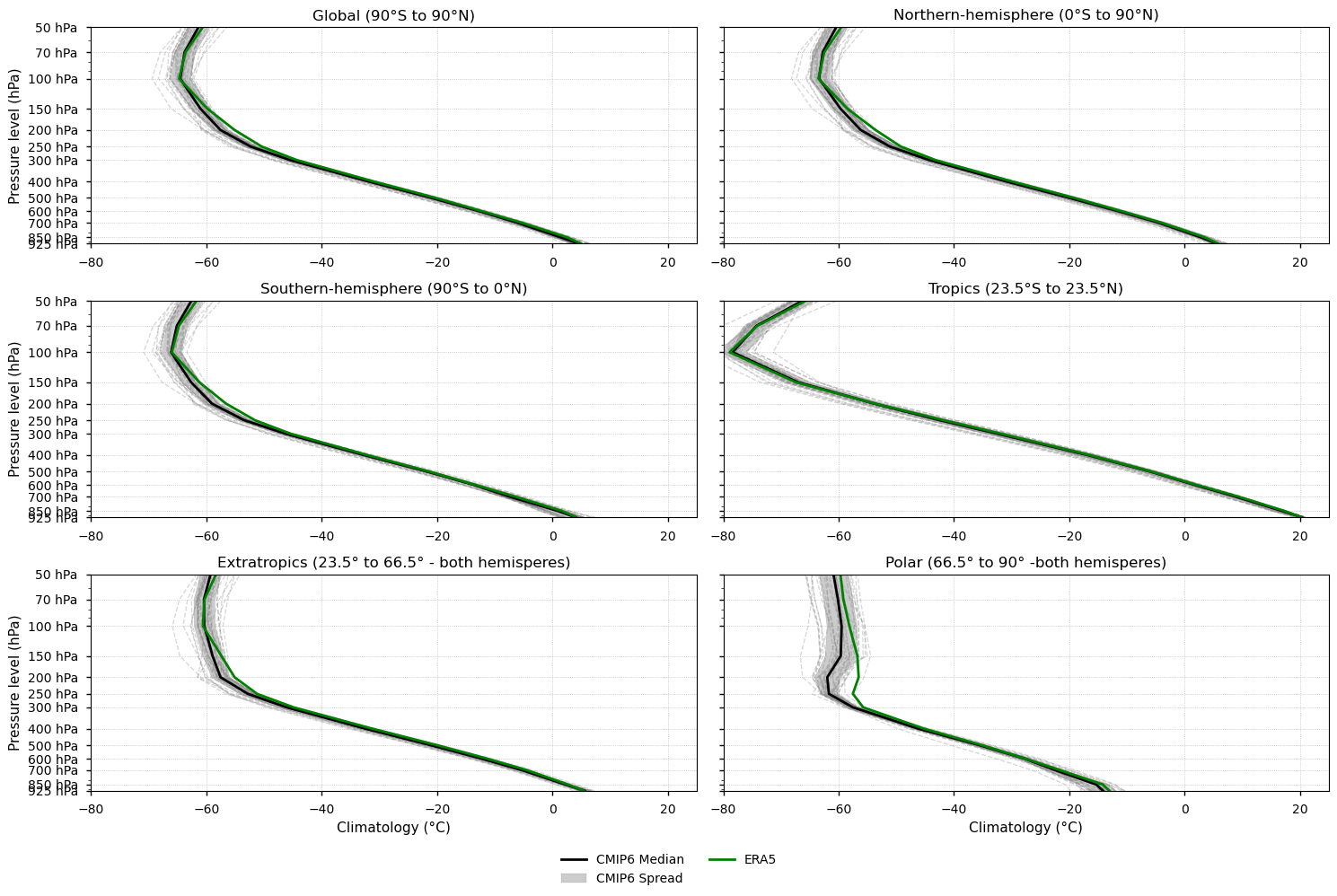
Fig 1. Vertical profiles of the annual mean temperature climatology (1979-2014). Each subplot shows a latitudinal band (Global, Northern and Southern hemispheres, Tropics, Extratropics, and Polar). ERA5 is shown as a green line, the CMIP6 median as a solid black line, individual CMIP6 models as grey dashed lines, and the spread of models as a grey shaded area.

3.3. Plot mean bias maps#

In this section, we invoke the plot_profile() function to display the vertical profiles of the mean bias for each latitudinal band, showing the median of the CMIP6 model biases and their spread.

../../_images/7c992ad088bf34756f94548e2101fdc651eab95f93d050ce38ab6a45e51ad6d1.png

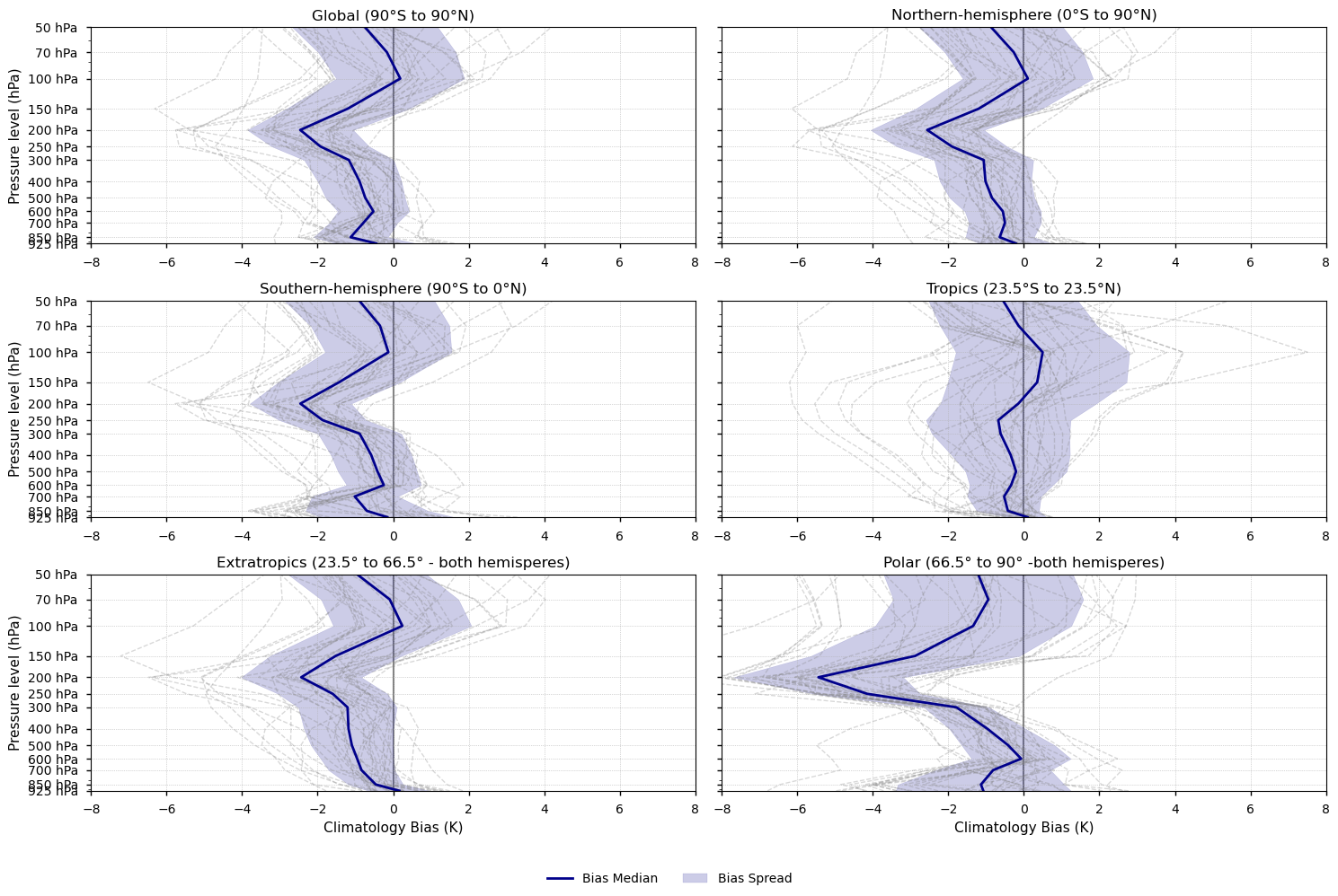
Fig 2. Vertical profiles of the mean bias of the annual mean temperature (1979-2014). Each subplot shows a latitudinal band (Global, Northern and Southern hemispheres, Tropics, Extratropics, and Polar). The CMIP6 median is shown as a solid blue line, individual CMIP6 models as grey dashed lines, and the spread of models as a blue shaded area.

3.4. Plot trend maps#

In this section, we invoke the plot_profile() function to display the vertical profiles of the trend for each latitudinal band, including ERA5, the median of the CMIP6 models, and the spread

../../_images/09fa312ba8712a8766da8385e766e0c5a25a2d8b659ab0253931987c9a5e67a9.png

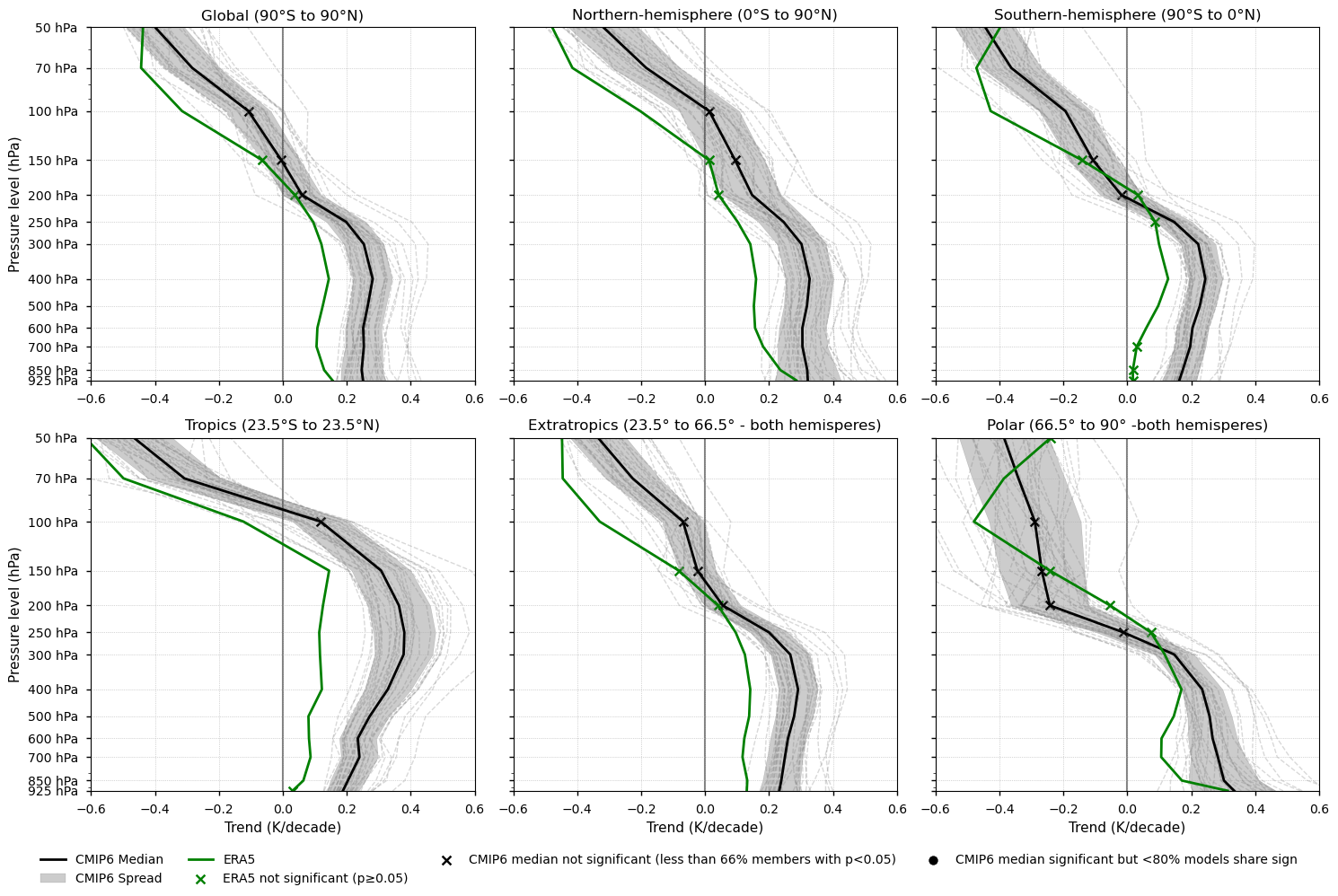
Fig 3. Vertical profiles of the annual mean temperature trend (1979-2014). Each subplot corresponds to a latitudinal band (Global, Northern Hemisphere, Southern Hemisphere, Tropics, Extratropics, and Polar). ERA5 is shown as a green line, the CMIP6 ensemble median as a solid black line, individual CMIP6 models as grey dashed lines, and the ensemble spread as a grey shaded area. ERA5 points with non-significant trends (p-value > 0.05) are marked with green crosses. For the CMIP6 ensemble median, trend significance is assessed using agreement categories based on the approach described in the IPCC AR6 Atlas (pp. 1945–1950). Black crosses indicate pressure levels where fewer than 66% of models show statistically significant trends (p-value < 0.05). If over 66% of the models are significant but fewer than 80% agree on the sign of the trend, a black dot is placed on the CMIP6 ensemble median to indicate low directional agreement.

3.5. Plot trend bias maps#

In this section, we invoke the plot_profile() function to display the vertical profiles of the trend bias for each latitudinal band, showing the median of the CMIP6 model biases and their spread.

../../_images/623b6b70497f5ce2fde7118cf3e86d39db71e1e6b6b41b3eaf09b68bcbdaa0fa.png

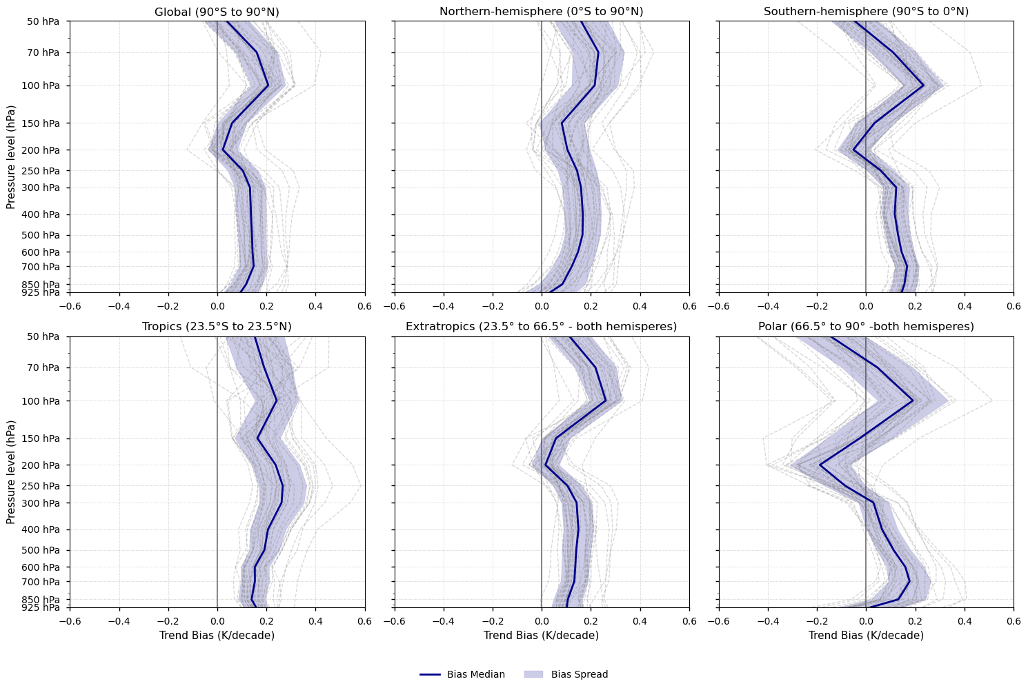
Fig 4. Vertical profiles of the trend bias of the annual mean temperature (1979-2014). Each subplot shows a latitudinal band (Global, Northern and Southern hemispheres, Tropics, Extratropics, and Polar). The CMIP6 median is shown as a solid blue line, individual CMIP6 models as grey dashed lines, and the spread of models as a blue shaded area.

3.6. Results summary and discussion - Climatologies#

Vertical temperature profiles are broadly consistent across latitudinal bands, with the tropopause—defined as the level where the temperature inversion begins—occurring at lower pressures in the tropics and higher pressures in colder regions (e.g. polar and extratropical).
Biases are predominantly cold, with the median of the model biases showing the largest discrepancies around 250–200 hPa, where CMIP6 models exhibit a sharper temperature transition than ERA5. Near-surface and stratospheric median biases are generally smaller, except in polar regions.
Model spread increases with altitude, particularly in the stratosphere, highlighting reduced inter-model agreement at higher levels.
The large spread near the tropopause underscores the substantial uncertainty in simulating its height and structure, which may have important implications for model evaluation and development.

3.7. Results summary and discussion - Trends#

Tropospheric warming and stratospheric cooling are robust signals of climate change consistent with greenhouse gas forcing. Both ERA5 and CMIP6 reproduce this behaviour across all latitudinal bands.
The vertical profile of temperature trends is a well-established fingerprint of climate change [3]. However, its magnitude and structure are highly sensitive to dataset-specific processing and homogenisation methods [6], limiting the robustness of long-term trend assessments.
As stated in IPCC AR5 [6]: “There is only medium to low confidence in the rate of change of tropospheric warming and its vertical structure. Estimates of tropospheric warming rates encompass surface temperature warming rate estimates.”
Tropical amplification—enhanced warming in the upper tropical troposphere relative to the surface—is evident in both ERA5 and CMIP6, although CMIP6 tends to show a stronger signal.
Amplification varies across latitudinal bands. CMIP6 models display amplification in all regions except the polar zones, whereas ERA5 shows amplification everywhere except in the polar and Northern Hemisphere bands, where warming is stronger near the surface. However, in the global and extratropical bands, both CMIP6 and ERA5 exhibit minimal amplification.
Differences between CMIP6 and ERA5 can be linked to biases in surface warming [8]. Studies using models with prescribed SSTs (e.g. [9]) report reduced biases. In addition, upper-troposphere trend estimates can vary depending on the analysis period, due to factors such as ozone changes.
Alternative reference datasets, such as RHARM available through the CDS, could have been used in this assessment. However, they may be better suited for regional to local-scale studies because, despite extensive harmonisation efforts [10], these datasets still exhibit residual inconsistencies—such as limited station coverage, short time series, and sensitivity to data selection criteria.
ERA5 is used as the reference dataset in this analysis to minimise temporal and vertical inhomogeneities, although it is not free from biases. Given the uncertainties associated with individual datasets, using multiple reference products—including those external to the CDS—would be advisable for this type of assessment. For example, [7] compared tropospheric and stratospheric trends using both ground- and satellite-based observations.

ℹ️ If you want to know more#

Key resources#

Some key resources and further reading were linked throughout this assessment.

The CDS catalogue entries for the data used were:

CMIP6 climate projections (Monthly - Air temperature): https://cds.climate.copernicus.eu/datasets/projections-cmip6?tab=overview
ERA5 monthly averaged data on pressure levels from 1940 to present (Temperature): https://cds.climate.copernicus.eu/datasets/reanalysis-era5-pressure-levels-monthly-means?tab=overview
ERA5 monthly averaged data on single levels from 1940 to present (Surface pressure): https://cds.climate.copernicus.eu/datasets/reanalysis-era5-single-levels-monthly-means?tab=overview

Code libraries used:

C3S EQC custom functions, c3s_eqc_automatic_quality_control, prepared by B-Open

References#

[1] Santer, B.D., Thorne, P.W., Haimberger, L., Taylor, K.E., Wigley, T.M.L., Lanzante, J.R., Solomon, S., Free, M., Gleckler, P.J., Jones, P.D., Karl, T.R., Klein, S.A., Mears, C., Nychka, D., Schmidt, G.A., Sherwood, S.C. and Wentz, F.J., 2008. Consistency of modelled and observed temperature trends in the tropical troposphere. Int. J. Climatol., 28: 1703-1722. https://doi.org/10.1002/joc.1756

[2] Simon F. B. Tett et al., 1996. Human Influence on the Atmospheric Vertical Temperature Structure: Detection and Observations.Science274,1170-1173. https://doi.org/10.1126/science.274.5290.1170

[3] Santer, B.D., Painter, J.F., Bonfils, C., Mears, C.A., Solomon, S., Wigley, T.M.L., Gleckler,P.J., Schmidt, G.A., Doutriaux,C., Gillett, N.P., Taylor,K.E., Thorne, P.W., and Wentz, F.J., 2013. Human and natural influences on the changing thermal structure of the atmosphere, Proc. Natl. Acad. Sci. U.S.A. 110 (43) 17235-17240. https://doi.org/10.1073/pnas.1305332110

[4] B. D. Santer et al., 2005. Amplification of Surface Temperature Trends and Variability in the Tropical Atmosphere.Science309,1551-1556. https://doi.org/10.1126/science.1114867

[5] Stone, P. H., and Carlson, J. H., 1979. Atmospheric lapse rate regimes and their parameterization. J. Atmos. Sci., 36, 415–423. https://doi.org/10.1175/1520-0469(1979)036<0415:ALRRAT>2.0.CO;2 .

[6] Hartmann, D. L., et al., 2013. Observations: Atmosphere and surface. Climate Change 2013: The Physical Science Basis, T. F. Stocker et al., Eds., Cambridge University Press, 159–254.

[7] Steiner, A. K. et al., 2020. Observed Temperature Changes in the Troposphere and Stratosphere from 1979 to 2018. J. Climate, 33, 8165–8194, https://doi.org/10.1175/JCLI-D-19-0998.1

[8] Mitchell, D. M., Thorne, P. W., Stott, P. A., and Gray, L. J., 2013. Revisiting the controversial issue of tropical tropospheric temperature trends, Geophys. Res. Lett., 40, 2801–2806, https://doi.org/10.1002/grl.50465

[9] Dann M. Mitchell et al., 2020. The vertical profile of recent tropical temperature trends: Persistent model biases in the context of internal variability. Environ. Res. Lett. 15 1040b4. https://doi.org/10.1088/1748-9326/ab9af7

[10] Madonna, F., Tramutola, E., SY, S., Serva, F., Proto, M., Rosoldi, M., et al., 2022. The new Radiosounding HARMonization (RHARM) data set of homogenized radiosounding temperature, humidity, and wind profiles with uncertainties. Journal of Geophysical Research: Atmospheres, 127, e2021JD035220. https://doi.org/10.1029/2021JD035220