

5.2.1. Assessing CORDEX temperature biases in the Alpine region through comparison with CERRA and E-OBS to support ski and hydrological sectors.#
Production date: 30-06-2025
Produced by: CMCC foundation - Euro-Mediterranean Center on Climate Change. Albert Martinez Boti and Lorenzo Sangelantoni.
🌍 Use case: Investigating climate biases in mountain regions to inform the ski and hydrological sectors.#
❓ Quality assessment question#
Do the cold biases commonly found in Regional Climate Models over the Alps persist when evaluated against CERRA?
Does applying a lapse-rate correction systematically reduce these biases?
Mountains, although covering a limited land area, are vital to the global water cycle, acting as key sources of freshwater for both ecological and human needs [1]. In many mountainous regions, temperature is a critical driver of hydrometeorological processes such as the ratio of rain to snow, the timing of snowmelt, and the frequency of low-flow conditions [2]. These sensitivities make mountain regions key indicators of climate change. However, accurately representing temperature in complex terrain remains challenging for models due to factors like topographic variability, slope orientation, terrain shading, snow–albedo feedbacks, and vegetation heterogeneity [2]).
A recent literature-based quality assessment, CORDEX temperature biases over the Alpine region for the ski and hydrological sectors), synthesised multiple studies and confirmed that many Regional Climate Models (RCMs) exhibit persistent cold biases over the Alps despite their relatively high resolution and improved representation of physical processes in mountainous terrain. The findings of the assessment also highlight the sensitivity of bias estimates to the choice of reference dataset [3][4]. In this analysis, we assess whether these cold biases persist when RCM outputs are evaluated against CERRA, a high-resolution (5.5 km) regional reanalysis produced using the HARMONIE-ALADIN limited-area numerical weather prediction and data assimilation system. To place CERRA into context, we also compare results against E-OBS, a widely used gridded observational dataset, to evaluate consistency across reference products. The analysis includes a broad ensemble of EURO-CORDEX models and examines the altitude dependency of biases by evaluating results across different elevation bands. Additionally, we investigate whether applying a lapse-rate correction systematically improves model performance relative to E-OBS.
📢 Quality assessment statement#
These are the key outcomes of this assessment
RCMs show systematic cold biases above 1000–1500 m, especially in winter and for cold extremes, which may affect snow and water-related planning.
Large inter-model spread—especially for winter cold extremes above 2000 m—highlights significant uncertainty in representing conditions critical for alpine risk assessments.
Compared to E-OBS, CERRA shows strong winter cold deviations at high elevations, suggesting it may not reliably represent mountain climates despite its high resolution.
Uncertainty in the E-OBS reference product—due to sparse high-altitude station coverage, complex terrain, and interpolation limitations—can contribute to apparent model biases, especially for temperature extremes in mountainous regions. Users should interpret comparisons with E-OBS cautiously, acknowledging that some biases may reflect observational data uncertainties rather than model deficiencies.
Lapse-rate adjustments reduce elevation mismatches but do not fix the overall vertical bias structure in RCMs.
The findings of this Alpine-focused assessment highlight the need for caution when interpreting future temperature projections from RCMs. A central concern is the potential for present-climate biases to persist or propagate into future warming scenarios—an aspect that remains largely underexplored.
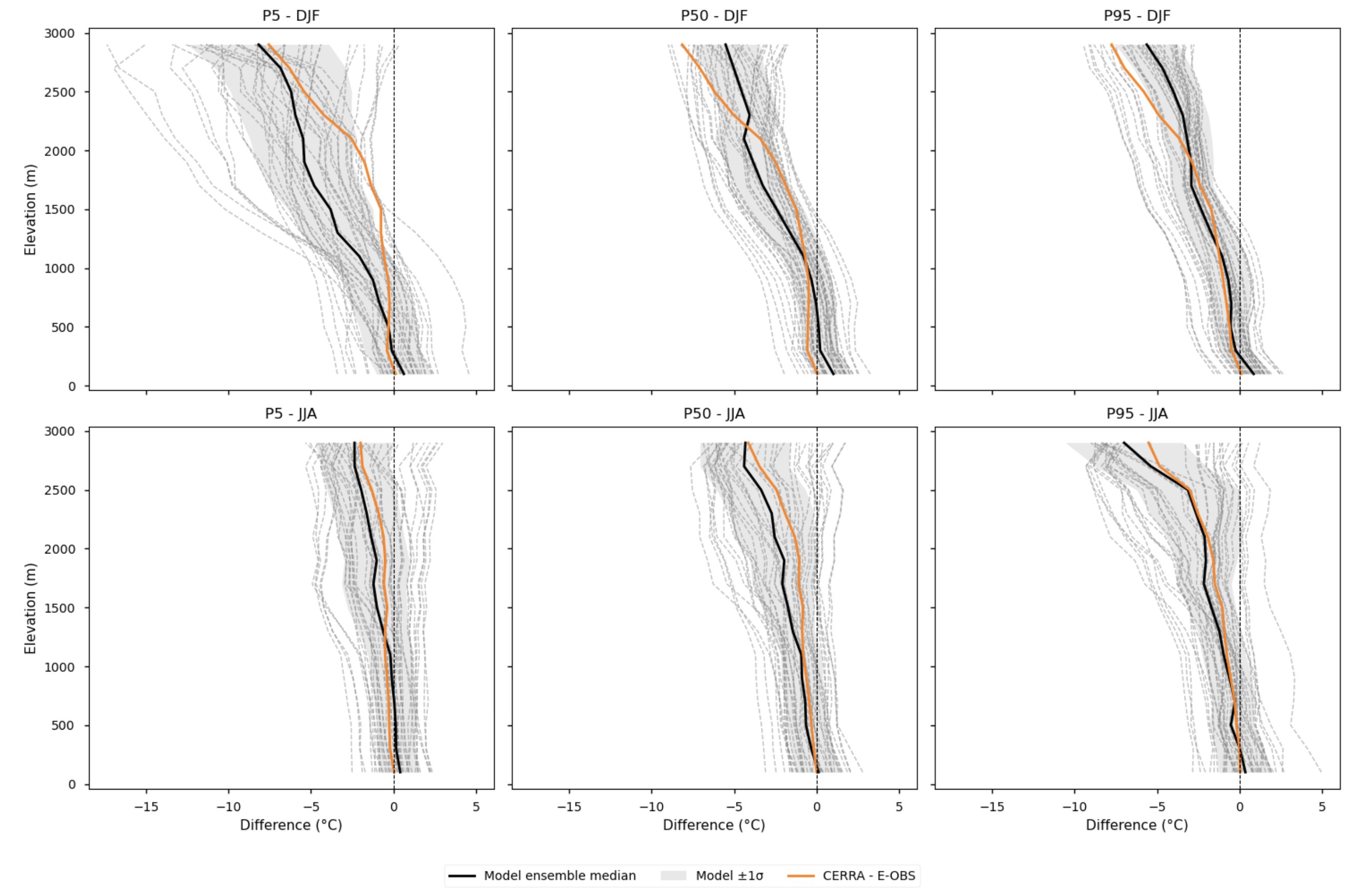
Fig. 5.2.1.1 Elevation profiles of biases relative to E-OBS. Differences compared to the E-OBS vertical profile are shown for each EURO-CORDEX model individually, the ensemble median, the spread (calculated as the standard deviation), and CERRA. Profiles are plotted separately for winter (DJF) and summer (JJA), and for the 5th, 50th, and 95th percentiles. The ensemble median is represented by a solid black line, while individual EURO-CORDEX models appear as grey dashed lines. The model spread, calculated as the standard deviation across models, is shown as a grey shaded area. CERRA is depicted in orange. No lapse-rate correction is applied in this case.#
📋 Methodology#
A subset of 39 models from EURO-CORDEX is compared to E-OBSv30.0e to assess the elevation dependency of temperature biases. Following the approach of [3], we evaluate differences between the RCMs and E-OBS in representing the 5th, 50th, and 95th percentiles of temperature at various altitude ranges, for both summer and winter, across the Greater Alpine Region (GAR; 4–19°E, 43–49°N, 0–3500 m a.s.l.; [5][6]). The extent of the GAR domain can be seen in Figure .2 reproduced from Haslinger et al., 2019 [5] under the CC BY 4.0.
To assess consistency across reference datasets, CERRA—a high-resolution (5.5 km) regional reanalysis produced using the HARMONIE-ALADIN limited-area numerical weather prediction and data assimilation system—is also compared to E-OBS and the RCMs.
All data are regridded to the 0.11° grid of a selected RCM (user-defined), which may introduce discrepancies due to differences in resolution, grid structure, and underlying orography—particularly when comparing to CERRA. To account for potential artefacts introduced by these differences, and to evaluate whether they contribute significantly to the observed biases, we also assess the effect of applying an elevation correction. This correction assumes a spatially and temporally uniform lapse rate of 0.0065 °C m⁻¹ and is applied to all regridded datasets—including CERRA, E-OBS, and the other RCMs—to adjust temperatures to the elevation of the model grid used for remapping, following a similar approach to [7].
The analysis and results follow the next outline:
1. Parameters, requests and functions definition
3.3. Elevation profiles of biases after applying lapse-rate correction
3.4. Elevation profiles of the impact of lapse-rate correction
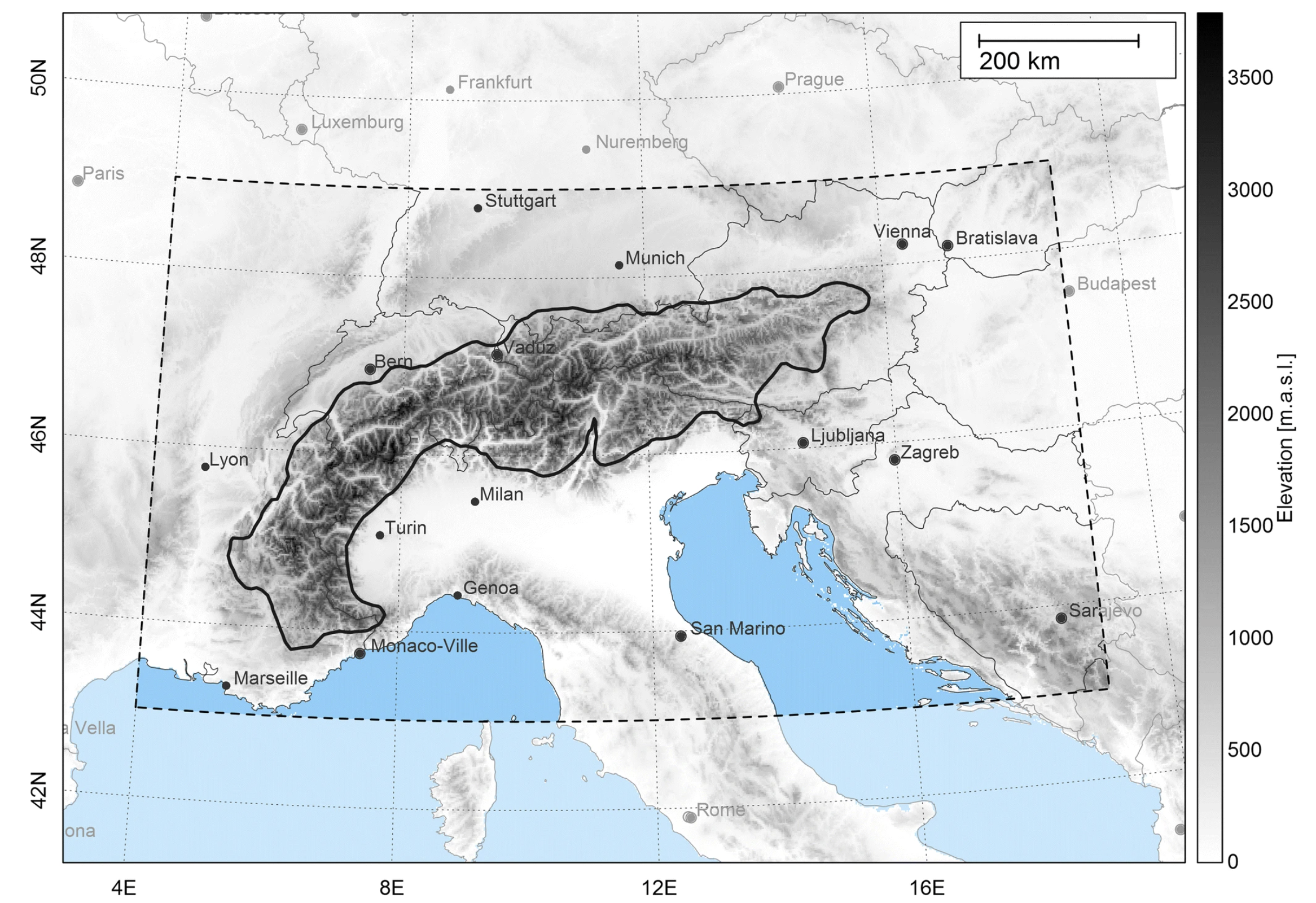
Fig. 5.2.1.2 Map of Central and Southern Europe. The broken line indicates the boundaries of the Greater Alpine Region; the solid line represents a generalized outline of the 1000 m a.s.l. isoline of the Alps which should help in locating the mountainous areas of the domain in the following figures. Image reproduced from Figure 1 in Haslinger et al., 2019 [5], under the CC BY 4.0#
📈 Analysis and results#
1. Parameters, requests and functions definition#
1.1. Import packages#
Show code cell source
import math
import tempfile
import warnings
import textwrap
warnings.filterwarnings("ignore")


import cartopy.crs as ccrs
import numpy as np
import matplotlib.pyplot as plt
import xarray as xr
import pandas as pd
from c3s_eqc_automatic_quality_control import diagnostics, download, plot, utils
import matplotlib.dates as mdates
from xarrayMannKendall import Mann_Kendall_test
from scipy.stats import linregress
from cartopy.mpl.gridliner import Gridliner
import scipy.signal as signal

plt.style.use("seaborn-v0_8-notebook")
plt.rcParams["hatch.linewidth"] = 0.5
1.2. Define Parameters#
In the “Define Parameters” section, various customisable options for the notebook are specified:
The start and end years of the historical period can be specified using the
year_startandyear_stopparameters. The default period, 1986–2005, is selected to maximise dataset availability while avoiding the need to include future projection data.The
chunkselection allows the user to define if dividing into chunks when downloading the data on their local machine. Although it does not significantly affect the analysis, it is recommended to keep the default value for optimal performance.variableandcollection_idare not customisable for this assessment and are set to ‘temperture’ and ‘CORDEX’. Expert users can use this notebook as a guide to create similar analyses for other variables or model sets.areadefines the geographical domain over which the analysis will be performed. Note that this notebook is designed for the EURO-CORDEX domain, so the selected area must lie within its boundaries. The Greater Alpine Region (GAR; 4–19°E, 43–49°N, 0–3500 m a.s.l.; [5][6]) is choosen for this assessment.rcm_model_regridandgcm_driven_model_regridspecify the EURO-CORDEX regional climate model and the driving global climate model, respectively, whose grid will be used as the target for remapping. Note that both models must be included in the matrix of RCM-GCM combinations defined by themodels_cordexdictionary in Section 1.3.
Show code cell source
# Time period
year_start = 1986
year_stop = 2005
assert year_start >= 1986

# Variable
variable = "temperature"
assert variable in ("temperature")

# Choose CORDEX or CMIP6
collection_id = "CORDEX"
assert collection_id in ("CORDEX")

# Area to show (Alpine Area)
area = [49, 4, 43, 19]
chunks = {"year": 1}

gcm_driven_model_regrid="ichec_ec_earth"
rcm_model_regrid="smhi_rca4"
1.3. Define models#
The following climate analyses are conducted using the EURO-CORDEX models available at the time of download, limited to those that include the orography variable in the Climate Data Store (CDS).
Show code cell source
gcm_models = (
    "cccma_canesm2","cnrm_cerfacs_cm5","ichec_ec_earth",
    "ipsl_cm5a_mr","miroc_miroc5", "mohc_hadgem2_es",
    "mpi_m_mpi_esm_lr", "ncc_noresm1_m"
)
models_r1i1p1_orog=["cnrm_aladin63","dmi_hirham5","mohc_hadrem3_ga7_05","knmi_racmo22e"]
model_regrid=f"{gcm_driven_model_regrid}_{rcm_model_regrid}"

models_cordex={
    "cccma_canesm2":["gerics_remo2015"],
    "cnrm_cerfacs_cm5":("clmcom_eth_cosmo_crclim","cnrm_aladin63","dmi_hirham5",
                        "gerics_remo2015",
                        "knmi_racmo22e","mohc_hadrem3_ga7_05"),
    "ichec_ec_earth":("clmcom_eth_cosmo_crclim","dmi_hirham5",
                     "knmi_racmo22e","smhi_rca4"),
    "ipsl_cm5a_mr":("dmi_hirham5","gerics_remo2015",
                   "knmi_racmo22e","smhi_rca4"),
    "miroc_miroc5":("clmcom_clm_cclm4_8_17","gerics_remo2015"),
    "mohc_hadgem2_es":("clmcom_clm_cclm4_8_17",
                      "cnrm_aladin63","dmi_hirham5","gerics_remo2015",
                      "knmi_racmo22e",
                       "mohc_hadrem3_ga7_05","smhi_rca4"),
    "mpi_m_mpi_esm_lr":("clmcom_clm_cclm4_8_17","clmcom_eth_cosmo_crclim",
                       "cnrm_aladin63","dmi_hirham5",
                        "knmi_racmo22e","mohc_hadrem3_ga7_05",
                       "mpi_csc_remo2009","smhi_rca4","uhoh_wrf361h"),
    "ncc_noresm1_m":("cnrm_aladin63","dmi_hirham5",
                    "gerics_remo2015",
                     "knmi_racmo22e","mohc_hadrem3_ga7_05","smhi_rca4"),
}

resample_reduction = "mean"
cerra_variable = "2m_temperature"
eobs_variable="mean_temperature"
cordex_variable = "2m_air_temperature"
1.4. Define CERRA request#
Within this notebook, CERRA is compared to E-OBS to evaluate differences across reference datasets. In this section, we set the required parameters for the cds-api data-request of CERRA.
Show code cell source
request_cerra = (

    "reanalysis-cerra-single-levels",
    {
        "data_type": ["reanalysis"],
        "product_type": "analysis",
        "data_format": "netcdf",
        "variable": [cerra_variable],
        "level_type": "surface_or_atmosphere",
        "year": [
            str(year)
            for year in range(year_start, year_stop + 1)
        ],  # Include D(year-1)
        "month": [f"{month:02d}" for month in range(1, 13)],
        "day": [f"{day:02d}" for day in range(1, 32)],
        "time": [
            "00:00", "03:00", "06:00",
            "09:00", "12:00", "15:00",
            "18:00", "21:00"],
    },
)

request_orography_cerra=(
    "reanalysis-cerra-single-levels",
    [
        {
            "variable": ["orography"],
            "level_type": "surface_or_atmosphere",
            "data_type": ["reanalysis"],
            "product_type": "analysis",
            "year": ["1987"],
            "month": ["01"],
            "day": ["01"],
            "time": ["00:00"],
            "data_format": "netcdf"
        }
    ]
)
1.5. Define E-OBS request#
Within this notebook, E-OBS serves as the reference product. In this section, we set the required parameters for the cds-api data-request of E-OBS.
Show code cell source
request_eobs = (
    "insitu-gridded-observations-europe",
    {
        "product_type": "ensemble_mean",
        "variable": [eobs_variable],
        "grid_resolution": "0_1deg",
        "period": ["1980_1994","1995_2010"],
        "version": ["30_0e"]
    },
)

request_orography_eobs = (
    "insitu-gridded-observations-europe",
    {
        "product_type": "elevation",
        "variable": ["land_surface_elevation"],
        "grid_resolution": "0_1deg",
        "period":"full_period",
        "version": ["30_0e"]
    },
)

request_lsm = (
    request_cerra[0],
    request_cerra[1]
    | {
        "year": "1986",
        "month": "01",
        "day": "01",
        "time": "00:00",
        "variable": "land_sea_mask",
    },
)
1.6. Define model requests#
In this section we set the required parameters for the cds-api data-request of EURO-CORDEX models.
Show code cell source
request_cordex = {
    "format": "zip",
    "domain": "europe",
    "experiment": "historical",
    "horizontal_resolution": "0_11_degree_x_0_11_degree",
    "temporal_resolution": "daily_mean",
    "variable": [cordex_variable],
    "ensemble_member": "r1i1p1",
}

def get_cordex_years(
    year_start,
    year_stop,
    start_years=list(range(1951, 2097, 5)),
    end_years=list(range(1955, 2101, 5)),
):
    start_year = []
    end_year = []
    years = set(range(year_start, year_stop + 1))
    for start, end in zip(start_years, end_years):
        if years & set(range(start, end + 1)):
            start_year.append(start)
            end_year.append(end)
    return start_year, end_year


model_requests = {}

for gcm_model in gcm_models:
    for model in models_cordex[gcm_model]:
        start_years = list(range(year_start, year_stop+1, 5))
        end_years = list(range(year_start+4, year_stop+5, 5))
        model_requests[f"{gcm_model}_{model}"] = (
            "projections-cordex-domains-single-levels",
            [
                {
                    "rcm_model": model,
                    "gcm_model": gcm_model,
                    **request_cordex,
                    "start_year": [str(start_year)],
                    "end_year": [str(end_year)],
                }
                for start_year, end_year in zip(
                    *get_cordex_years(
                        year_start,
                        year_stop,
                        start_years=start_years,
                        end_years=end_years,
                    )
                )
            ],
        )

request_grid_out = model_requests[model_regrid]

request_orography_grid_out=(
    "projections-cordex-domains-single-levels",
    [
        {
            "domain": "europe",
            "experiment": "historical",
            "horizontal_resolution": "0_11_degree_x_0_11_degree",
            "temporal_resolution": "fixed",
            "variable": ["orography"],
            "gcm_model": gcm_driven_model_regrid,
            "rcm_model": rcm_model_regrid,
            "ensemble_member": "r0i0p0",
        }
    ]
)

model_requests_orography = {}

for gcm_model in gcm_models:
    for model in models_cordex[gcm_model]:
        gcm_rcm_combination=f"{gcm_model}_{model}"
        model_requests_orography[gcm_rcm_combination]=(
            "projections-cordex-domains-single-levels",
            [
                {
                    "domain": "europe",
                    "experiment": "rcp_8_5" if gcm_rcm_combination in ["mpi_m_mpi_esm_lr_uhoh_wrf361h","ncc_noresm1_m_cnrm_aladin63"] else "historical",
                    "horizontal_resolution": "0_11_degree_x_0_11_degree",
                    "temporal_resolution": "fixed",
                    "variable": ["orography"],
                    "gcm_model": gcm_model,
                    "rcm_model": model,
                    "ensemble_member":"r1i1p1" if model in models_r1i1p1_orog else "r0i0p0",
                }
            ]
        )
1.7. Functions to cache#
In this section, functions that will be executed in the caching phase are defined. Caching is the process of storing copies of files in a temporary storage location, so that they can be accessed more quickly. This process also checks if the user has already downloaded a file, avoiding redundant downloads.
Description of the main functions:
compute_percentiles: This function resamples data to daily frequency if needed (e.g., for hourly CERRA data), performs regridding to the target grid, selects the subregion of interest, and calculates the 5th, 50th, and 95th percentiles for summer and winter.orog_regrid: This function regrids the elevation data from the models, CERRA, and E-OBS onto the target grid, enabling the subsequent application of a point-by-point lapse rate correction.
Show code cell source
def select_timeseries(ds, timeseries="JJA", year_start=None, year_stop=None):
    if timeseries == "JJA":
        season_months = [6, 7, 8]
    elif timeseries == "DJF":
        season_months = [12, 1, 2]
    else:
        raise ValueError(f"Unsupported season: {timeseries}")

    # Ensure time is datetime type
    time = ds.indexes["time"]
    if not np.issubdtype(time.dtype, np.datetime64):
        ds["time"] = xr.decode_cf(ds).time

    # Filter by years
    ds = ds.sel(time=slice(f"{year_start}-01-01", f"{year_stop}-12-31"))

    # Filter by season
    ds_season = ds.where(ds["time.month"].isin(season_months), drop=True)
    return ds_season

def get_p(ds, percentile):
    return ds.quantile(percentile/100, dim="time", skipna=True)

def add_bounds(ds):
    for coord in {"latitude", "longitude"} - set(ds.cf.bounds):
        ds = ds.cf.add_bounds(coord)
    return ds

def get_grid_out(request_grid_out, method):
    ds_regrid = download.download_and_transform(*request_grid_out)
    coords = ["latitude", "longitude"]
    if method == "conservative":
        ds_regrid = add_bounds(ds_regrid)
        for coord in list(coords):
            coords.extend(ds_regrid.cf.bounds[coord])
    grid_out = ds_regrid[coords]
    coords_to_drop = set(grid_out.coords) - set(coords) - set(grid_out.dims)
    grid_out = ds_regrid[coords].reset_coords(coords_to_drop, drop=True)
    grid_out.attrs = {}
    return grid_out


def compute_percentiles(
    ds,
    year_start,
    year_stop,
    area,
    resample_reduction=None,
    request_grid_out=None,
    **regrid_kwargs,
):
    assert (request_grid_out and regrid_kwargs) or not (
        request_grid_out or regrid_kwargs
    )
    ds = ds.drop_vars([var for var, da in ds.data_vars.items() if len(da.dims) != 3])
    ds = ds[list(ds.data_vars)]
    ds=ds.convert_calendar('proleptic_gregorian', align_on='date', use_cftime=False)
    ds = ds.sel(time=slice(f"{year_start}-01-01", f"{year_stop}-12-31"))

    # Select a subdomain
    regionalise_kwargs = {
        "lon_slice": slice(area[1], area[3]),
        "lat_slice": slice(area[0], area[2]),
    }


    if resample_reduction:
        resampled = ds.resample(time="1D")
        ds = getattr(resampled, resample_reduction)(keep_attrs=True)

    # Original bounds for conservative interpolation
    if regrid_kwargs.get("method") == "conservative":
        ds = add_bounds(ds)
        bounds = [
            ds.cf.get_bounds(coord).reset_coords(drop=True)
            for coord in ("latitude", "longitude")
        ]
    else:
        bounds = []

    if request_grid_out:
        ds = diagnostics.regrid(
            ds.merge({da.name: da for da in bounds}),
            grid_out=get_grid_out(request_grid_out, regrid_kwargs["method"]),
            **regrid_kwargs,
        )
    ds = utils.regionalise(ds, **regionalise_kwargs)


    # Compute percentiles
    data_dict = {}
    for season in ["jja", "djf"]:
        ds_season = select_timeseries(
            ds, timeseries=season.upper(), year_start=year_start, year_stop=year_stop
        ).chunk({"time": -1})
        for p in [5, 50, 95]:
            key = f"p{p}_{season}"
            data_dict[key] = list(get_p(ds_season, p).data_vars.values())[0]


    ds= xr.merge([xr.Dataset({k: v}) for k, v in data_dict.items()], compat="override")
    return ds

def orog_regrid(
    ds,
    area,
    request_grid_out=None,
    **regrid_kwargs,
):
    # Select a subdomain
    regionalise_kwargs = {
        "lon_slice": slice(area[1], area[3]),
        "lat_slice": slice(area[0], area[2]),
    }
    # Original bounds for conservative interpolation
    if regrid_kwargs.get("method") == "conservative":
        ds = add_bounds(ds)
        bounds = [
            ds.cf.get_bounds(coord).reset_coords(drop=True)
            for coord in ("latitude", "longitude")
        ]
    else:
        bounds = []
    if request_grid_out:
        ds = diagnostics.regrid(
                ds.merge({da.name: da for da in bounds}),
                grid_out=get_grid_out(request_grid_out, regrid_kwargs["method"]),
                **regrid_kwargs,
            )
    ds = utils.regionalise(ds, **regionalise_kwargs)
    return ds
2. Downloading and processing#
2.1. Download and transform the regridding model#
In this section, the download.download_and_transform function from the c3s_eqc_automatic_quality_control package is employed to download daily data from the selected EURO-CORDEX regridding model, select the subregion of interest, and calculate the 5th, 50th, and 95th percentiles for summer and winter over the period 1986–2005, caching the results to avoid redundant downloads and processing. Elevation data for the selected model is also retrieved, as it is required to perform the lapse-rate correction.
The regridding model here refers to the model whose grid is used as the target grid for remapping the other models, as well as CERRA5 and E-OBS. This ensures all datasets share a common grid, facilitating direct comparison at each grid cell. Within this notebook, the regridding model is set to "ichec_ec_earth_smhi_rca4" but it can be changed by modifying the gcm_driven_model_regrid and rcm_model_regrid parameters in Section 1.2. Note that both models must be included in the matrix of RCM-GCM combinations defined by the models_cordex dictionary in Section 1.3. It is important to highlight that the choice of the target grid can significantly impact the analysis depending on the specific application.
Show code cell source
kwargs = {
    "chunks": None,
    "transform_chunks": False,
    "transform_func": compute_percentiles,
}
transform_func_kwargs = {
    "year_start": year_start,
    "year_stop": year_stop,
    "area": area,
}
ds_regrid = download.download_and_transform(
    *request_grid_out,
    **kwargs,
    transform_func_kwargs=transform_func_kwargs,
)

ds_orog_grid_out=download.download_and_transform(
    *request_orography_grid_out,
    chunks=None,
    transform_chunks=False,
    transform_func=orog_regrid,
    transform_func_kwargs={"area":area}
)
2.2. Download and transform CERRA#
In this section, the download.download_and_transform function from the c3s_eqc_automatic_quality_control package is used to download sub-daily data from CERRA (which is compared to E-OBS to evaluate differences between reference datasets in this notebook), resample it to daily frequency, regrid to the target grid, select the subregion of interest, and compute the 5th, 50th, and 95th percentiles for summer and winter over the period 1986–2005. The results are cached to avoid redundant downloads and processing. Elevation data is also retrieved and regridded to the target grid, as it is required to perform the lapse-rate correction.
Show code cell source
transform_func_kwargs = {
    "year_start": year_start,
    "year_stop": year_stop,
    "area": area,
}

transform_func_kwargs_orog = {
    "request_grid_out": request_orography_grid_out,
    "area": area,
}
ds_cerra = download.download_and_transform(
    *request_cerra,
    chunks=chunks,
    transform_chunks=False,
    transform_func=compute_percentiles,
    transform_func_kwargs=transform_func_kwargs
    | {
        "resample_reduction": resample_reduction,
        "request_grid_out": request_grid_out,
        "method": "bilinear",
        "skipna": True,
    },
)

ds_orog_cerra=download.download_and_transform(
    *request_orography_cerra,
    chunks=None,
    transform_chunks=False,
    transform_func=orog_regrid,
    transform_func_kwargs=transform_func_kwargs_orog|
        {
            "method": "bilinear",
            "skipna": True,
        }
).isel(time=0)
2.3. Download and transform E-OBS#
In this section, the download.download_and_transform function from the c3s_eqc_automatic_quality_control package is used to download sub-daily data from CERRA (which is compared to E-OBS to evaluate differences between reference datasets in this notebook), resample it to daily frequency, regrid to the target grid, select the subregion of interest, and compute the 5th, 50th, and 95th percentiles for summer and winter over the period 1986–2005. The results are cached to avoid redundant downloads and processing. Elevation data is also retrieved and regridded to the target grid, as it is required to perform the lapse-rate correction.
Show code cell source
ds_eobs = download.download_and_transform(
    *request_eobs,
    chunks=None,
    transform_chunks=False,
    transform_func=compute_percentiles,
    transform_func_kwargs=transform_func_kwargs
    | {
        "resample_reduction": resample_reduction,
        "request_grid_out": request_grid_out,
        "method": "bilinear",
        "skipna": True,
    },
)
ds_orog_eobs=download.download_and_transform(
    *request_orography_eobs,
    chunks=None,
    transform_chunks=False,
    transform_func=orog_regrid,
    transform_func_kwargs=transform_func_kwargs_orog|
        {
            "method": "bilinear",
            "skipna": True,
        }
)
2.4. Download and transform models#
In this section, the download.download_and_transform function from the c3s_eqc_automatic_quality_control package is used to download daily data from the selected EURO-CORDEX models, regrid to the target grid, select the subregion of interest, and compute the 5th, 50th, and 95th percentiles for summer and winter over the period 1986–2005. The results are cached to avoid redundant downloads and processing. Elevation data is also retrieved and regridded to the target grid, as it is required to perform the lapse-rate correction.
Show code cell source
datasets = []
datasets_orog=[]

model_kwargs = {
        "chunks": None,
        "transform_chunks": False,
        "transform_func":compute_percentiles,
}

for model, requests in model_requests.items():
    print(f"{model=}")
    ds = download.download_and_transform(
        *requests,
        **model_kwargs,
        transform_func_kwargs=transform_func_kwargs|
            {
                "request_grid_out": request_grid_out,
                "method": "bilinear",
                "skipna": True,
            },
    )
    ds_orog=download.download_and_transform(
        *model_requests_orography[model],
        chunks=None,
        transform_chunks=False,
        transform_func=orog_regrid,
        transform_func_kwargs=transform_func_kwargs_orog|
            {
                "method": "bilinear",
                "skipna": True,
            }
        )

    datasets.append(ds.expand_dims(model=[model]))
    datasets_orog.append(ds_orog.expand_dims(model=[model]))

ds_models = xr.concat(datasets, "model",coords='minimal', compat='override')
ds_orog_models=xr.concat(datasets_orog, "model",coords='minimal', compat='override')
model='cccma_canesm2_gerics_remo2015'
model='cnrm_cerfacs_cm5_clmcom_eth_cosmo_crclim'
model='cnrm_cerfacs_cm5_cnrm_aladin63'
model='cnrm_cerfacs_cm5_dmi_hirham5'
model='cnrm_cerfacs_cm5_gerics_remo2015'
model='cnrm_cerfacs_cm5_knmi_racmo22e'
model='cnrm_cerfacs_cm5_mohc_hadrem3_ga7_05'
model='ichec_ec_earth_clmcom_eth_cosmo_crclim'
model='ichec_ec_earth_dmi_hirham5'
model='ichec_ec_earth_knmi_racmo22e'
model='ichec_ec_earth_smhi_rca4'
model='ipsl_cm5a_mr_dmi_hirham5'
model='ipsl_cm5a_mr_gerics_remo2015'
model='ipsl_cm5a_mr_knmi_racmo22e'
model='ipsl_cm5a_mr_smhi_rca4'
model='miroc_miroc5_clmcom_clm_cclm4_8_17'
model='miroc_miroc5_gerics_remo2015'
model='mohc_hadgem2_es_clmcom_clm_cclm4_8_17'
model='mohc_hadgem2_es_cnrm_aladin63'
model='mohc_hadgem2_es_dmi_hirham5'
model='mohc_hadgem2_es_gerics_remo2015'
model='mohc_hadgem2_es_knmi_racmo22e'
model='mohc_hadgem2_es_mohc_hadrem3_ga7_05'
model='mohc_hadgem2_es_smhi_rca4'
model='mpi_m_mpi_esm_lr_clmcom_clm_cclm4_8_17'
model='mpi_m_mpi_esm_lr_clmcom_eth_cosmo_crclim'
model='mpi_m_mpi_esm_lr_cnrm_aladin63'
model='mpi_m_mpi_esm_lr_dmi_hirham5'
model='mpi_m_mpi_esm_lr_knmi_racmo22e'
model='mpi_m_mpi_esm_lr_mohc_hadrem3_ga7_05'
model='mpi_m_mpi_esm_lr_mpi_csc_remo2009'
model='mpi_m_mpi_esm_lr_smhi_rca4'
model='mpi_m_mpi_esm_lr_uhoh_wrf361h'
model='ncc_noresm1_m_cnrm_aladin63'
model='ncc_noresm1_m_dmi_hirham5'
model='ncc_noresm1_m_gerics_remo2015'
model='ncc_noresm1_m_knmi_racmo22e'
model='ncc_noresm1_m_mohc_hadrem3_ga7_05'
model='ncc_noresm1_m_smhi_rca4'
2.5. Apply land-sea mask#
This section applies a land–sea mask to all models, as well as to CERRA and E-OBS, to ensure consistency in the land-only analysis.
Show code cell source
lsm = download.download_and_transform(*request_lsm)["lsm"].squeeze(drop=True)

# Cutout
regionalise_kwargs = {
    "lon_slice": slice(area[1], area[3]),
    "lat_slice": slice(area[0], area[2]),
}
lsm = utils.regionalise(lsm, **regionalise_kwargs)

datasets = {
    "ds_models": ds_models,"ds_cerra":ds_cerra,"ds_eobs":ds_eobs,
    "ds_orog_models": ds_orog_models,"ds_orog_cerra": ds_orog_cerra,
    "ds_orog_eobs": ds_orog_eobs
}

for name in datasets:
    datasets[name] = datasets[name].where(
        diagnostics.regrid(lsm, ds_orog_grid_out, method="bilinear")
    )

ds_models = datasets["ds_models"]
ds_cerra = datasets["ds_cerra"]
ds_eobs = datasets["ds_eobs"]
ds_orog_models = datasets["ds_orog_models"]
ds_orog_cerra = datasets["ds_orog_cerra"]
ds_orog_eobs = datasets["ds_orog_eobs"]
ds_orog_eobs = ds_orog_eobs[["elevation"]].rename({"elevation": "orog"})
100%|██████████| 1/1 [00:00<00:00, 29.63it/s]
3. Plot and describe results#
This section will display the following results:
Elevation profiles of biases relative to E-OBS: Differences are shown for each EURO-CORDEX model individually, the ensemble median, the spread (calculated as the standard deviation), and CERRA. Profiles are plotted separately for winter (DJF) and summer (JJA), and for the 5th, 50th, and 95th percentiles.
Elevation profiles of biases relative to E-OBS: Differences compared to the E-OBS vertical profile are shown for each EURO-CORDEX model individually, the ensemble median, the spread (calculated as the standard deviation), and CERRA. Profiles are plotted separately for winter (DJF) and summer (JJA), and for the 5th, 50th, and 95th percentiles.
Elevation profiles of biases after applying lapse-rate correction: As above, this includes each EURO-CORDEX model, the ensemble median, the spread, and CERRA, for both seasons and selected percentiles, but after correcting for elevation using a uniform lapse rate.
Elevation profiles of the impact of lapse-rate correction: This shows the difference between the corrected and uncorrected profiles for CERRA, E-OBS, individual EURO-CORDEX models, the ensemble median, and the spread. Results are again disaggregated by season and percentile.
3.1. Define plotting functions#
The functions compute_elevation_profile, plot_differences_vs_eobs, plot_lapse_rate_impact and apply_lapse_rate_correction are used to generate and visualise the elevation-dependent biases of temperature. Specifically:
compute_elevation_profilecalculates the vertical (elevation-based) profiles of the 5th, 50th, and 95th percentiles for each dataset (EURO-CORDEX models, CERRA, and E-OBS), separately for winter (DJF) and summer (JJA).apply_lapse_rate_correctionadjusts the temperature values for elevation differences by applying a uniform lapse rate (−0.0065 °C m⁻¹), aligning the model and reference data to the elevation of the target grid.plot_differences_vs_eobsplots the differences (biases) between the elevation profiles of the EURO-CORDEX models and CERRA, relative to that of E-OBS, for each percentile and season.plot_lapse_rate_impacthighlights the change introduced by the lapse-rate correction, showing the difference between corrected and uncorrected profiles for each dataset.
In the plots, the ensemble median is represented by a solid black line, while individual EURO-CORDEX models appear as grey dashed lines. The model spread, calculated as the standard deviation across models, is shown as a grey shaded area. CERRA is depicted in orange. Finally, E-OBS is shown in blue, but only in the plots that assess the impact of the lapse-rate correction.
Show code cell source
def compute_elevation_profile(da, ds_orog, elev_bins=np.arange(0, 3050, 200), kelvin_to_celsius=True,trend=False):
    if trend==False:
        if kelvin_to_celsius:
            da = da - 273.15
    else:
        factor = 3.15576e17
        da=da*factor
    values = da.values.flatten()
    elev = ds_orog["orog"].values.flatten()
    valid = ~np.isnan(values) & ~np.isnan(elev)
    values = values[valid]
    elev = elev[valid]
    elev_labels = (elev_bins[:-1] + elev_bins[1:]) / 2
    df = pd.DataFrame({'value': values, 'elev': elev})
    df['elev_bin'] = pd.cut(df['elev'], bins=elev_bins, labels=elev_labels)

    return df.groupby('elev_bin')['value'].mean()


def plot_differences_vs_eobs(ds_models_interpolated, ds_cerra, ds_eobs, ds_orog):
    fig, axs = plt.subplots(2, 3, figsize=(15, 10), sharex=True, sharey=True)
    percentiles = ["p5", "p50", "p95"]
    seasons = ["djf", "jja"]

    model_names = ds_models_interpolated.model.values
    elev_bins = np.arange(0, 3050, 200)
    elev_labels = (elev_bins[:-1] + elev_bins[1:]) / 2

    for i, season in enumerate(seasons):
        for j, p in enumerate(percentiles):
            varname = f"{p}_{season}"
            ax = axs[i, j]

            # Compute E-OBS and CERRA profiles
            profile_eobs = compute_elevation_profile(ds_eobs[varname], ds_orog, kelvin_to_celsius=False)
            profile_cerra = compute_elevation_profile(ds_cerra[varname], ds_orog)

            # Store model differences
            model_diffs = []

            for model in model_names:
                da_model = ds_models_interpolated[varname].sel(model=model)
                profile_model = compute_elevation_profile(da_model, ds_orog)
                diff_model = profile_model - profile_eobs
                model_diffs.append(diff_model)

                ax.plot(
                    diff_model.values,
                    diff_model.index.astype(float),
                    linestyle="--",
                    color="grey",
                    alpha=0.5,
                    linewidth=1
                )

            # Convert to DataFrame for ensemble stats
            df_models = pd.DataFrame(model_diffs, index=model_names)
            median_diff = df_models.median(axis=0)
            std_diff = df_models.std(axis=0)


            # Plot ensemble median
            ax.plot(
                median_diff.values,
                median_diff.index.astype(float),
                color="black",
                label="Model ensemble median",
                linewidth=2
            )
            # Plot ensemble spread
            ax.fill_betweenx(
                median_diff.index.astype(float),
                (median_diff - std_diff).values,
                (median_diff + std_diff).values,
                color="lightgrey",
                alpha=0.5,
                label="Model ±1σ" if i == 0 and j == 0 else None
            )


            # Plot CERRA - EOBS
            diff_cerra = profile_cerra - profile_eobs
            ax.plot(
                diff_cerra.values,
                diff_cerra.index.astype(float),
                color="tab:orange",
                label="CERRA - E-OBS",
                linewidth=2
            )

            # Formatting
            ax.axvline(0, color="k", linestyle="--", linewidth=0.8)
            ax.set_title(f"{p.upper()} - {season.upper()}")
            if j == 0:
                ax.set_ylabel("Elevation (m)")
            if i == 1:
                ax.set_xlabel("Difference (°C)")

    # Shared legend
    handles, labels = axs[0, 0].get_legend_handles_labels()
    fig.legend(handles, labels, loc="lower center", ncol=3)
    plt.tight_layout(rect=[0, 0.05, 1, 1])
    plt.show()

def apply_lapse_rate_correction(ds, ds_orog_native, ds_orog_target, lapse_rate=-0.0065, varnames=None):
    corrected = ds.copy()
    if varnames is None:
        varnames = list(ds.data_vars)

    delta_z = ds_orog_target["orog"] - ds_orog_native["orog"]

    for var in varnames:
        corrected[var] = ds[var] + lapse_rate * delta_z

    return corrected

def plot_lapse_rate_impact(ds_models_interpolated, ds_cerra, ds_eobs,
                           ds_models_interpolated_corr, ds_cerra_corr,
                           ds_eobs_corr, ds_orog):
    fig, axs = plt.subplots(2, 3, figsize=(15, 10), sharex=True, sharey=True)
    percentiles = ["p5", "p50", "p95"]
    seasons = ["djf", "jja"]

    model_names = ds_models_interpolated.model.values
    elev_bins = np.arange(0, 3050, 200)
    elev_labels = (elev_bins[:-1] + elev_bins[1:]) / 2

    for i, season in enumerate(seasons):
        for j, p in enumerate(percentiles):
            varname = f"{p}_{season}"
            ax = axs[i, j]

            # --- Compute difference: corrected - original ---
            # E-OBS
            profile_eobs_before = compute_elevation_profile(ds_eobs[varname], ds_orog, kelvin_to_celsius=False)
            profile_eobs_after = compute_elevation_profile(ds_eobs_corr[varname], ds_orog, kelvin_to_celsius=False)
            diff_eobs = profile_eobs_after - profile_eobs_before

            # CERRA
            profile_cerra_before = compute_elevation_profile(ds_cerra[varname], ds_orog)
            profile_cerra_after = compute_elevation_profile(ds_cerra_corr[varname], ds_orog)
            diff_cerra = profile_cerra_after - profile_cerra_before

            # Models
            model_diffs = []
            for model in model_names:
                profile_model_before = compute_elevation_profile(ds_models_interpolated[varname].sel(model=model), ds_orog)
                profile_model_after = compute_elevation_profile(ds_models_interpolated_corr[varname].sel(model=model), ds_orog)
                diff_model = profile_model_after - profile_model_before
                model_diffs.append(diff_model)

                # Plot individual model differences
                ax.plot(
                    diff_model.values,
                    diff_model.index.astype(float),
                    linestyle="--",
                    color="grey",
                    alpha=0.5,
                    linewidth=1
                )

            # Ensemble statistics
            df_models = pd.DataFrame(model_diffs, index=model_names)
            median_diff = df_models.median(axis=0)
            std_diff = df_models.std(axis=0)

            # Plot ensemble median
            ax.plot(
                median_diff.values,
                median_diff.index.astype(float),
                color="black",
                label="Model ensemble median",
                linewidth=2
            )
            # Plot ±1σ spread
            ax.fill_betweenx(
                median_diff.index.astype(float),
                (median_diff - std_diff).values,
                (median_diff + std_diff).values,
                color="lightgrey",
                alpha=0.5,
                label="Model ±1σ" if i == 0 and j == 0 else None
            )

            # Plot CERRA correction effect
            ax.plot(
                diff_cerra.values,
                diff_cerra.index.astype(float),
                color="tab:orange",
                label="CERRA",
                linewidth=2
            )

            # Plot E-OBS correction effect
            ax.plot(
                diff_eobs.values,
                diff_eobs.index.astype(float),
                color="tab:blue",
                label="E-OBS",
                linewidth=2
            )

            # Formatting
            ax.axvline(0, color="k", linestyle="--", linewidth=0.8)
            ax.set_title(f"{p.upper()} - {season.upper()}")
            if j == 0:
                ax.set_ylabel("Elevation (m)")
            if i == 1:
                ax.set_xlabel("ΔT (°C, lapse rate corrected − uncorrected)")


    # Shared legend
    handles, labels = axs[0, 0].get_legend_handles_labels()
    fig.legend(handles, labels, loc="lower center", ncol=3)
    plt.tight_layout(rect=[0, 0.05, 1, 1])
    plt.show()
3.2.Elevation profiles of biases relative to E-OBS#
Differences compared to the E-OBS vertical profile are shown for each EURO-CORDEX model individually, the ensemble median, the spread (calculated as the standard deviation), and CERRA. Profiles are plotted separately for winter (DJF) and summer (JJA), and for the 5th, 50th, and 95th percentiles.
Note that no lapse-rate correction is applied in this case, and data are grouped by altitude using the elevation of the target grid model.
Show code cell source
plot_differences_vs_eobs(ds_models, ds_cerra, ds_eobs, ds_orog_grid_out)
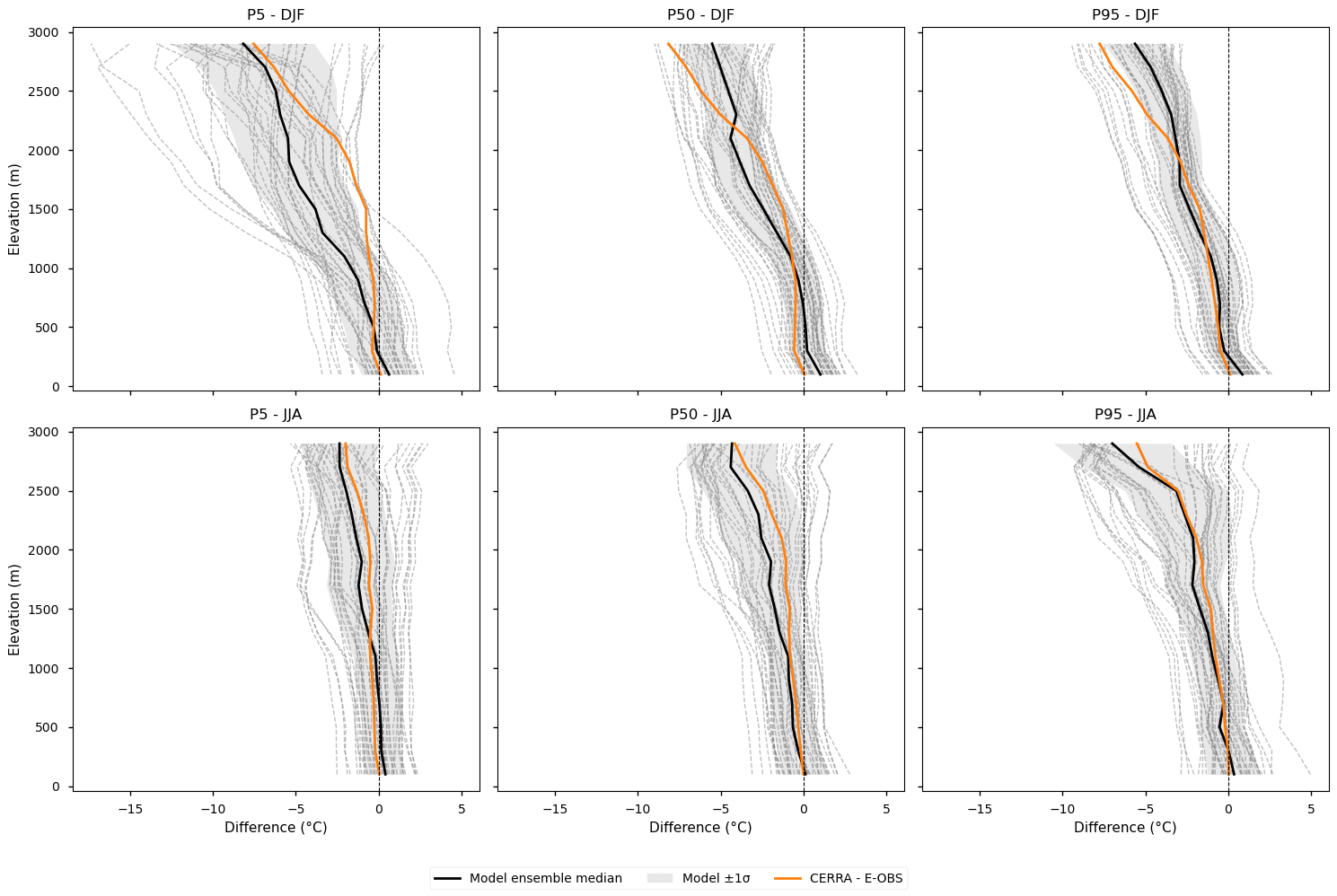
Fig 3. Elevation profiles of biases relative to E-OBS. Differences compared to the E-OBS vertical profile are shown for each EURO-CORDEX model individually, the ensemble median, the spread (calculated as the standard deviation), and CERRA. Profiles are plotted separately for winter (DJF) and summer (JJA), and for the 5th, 50th, and 95th percentiles. The ensemble median is represented by a solid black line, while individual EURO-CORDEX models appear as grey dashed lines. The model spread, calculated as the standard deviation across models, is shown as a grey shaded area. CERRA is depicted in orange. No lapse-rate correction is applied in this case.
3.3. Elevation profiles of biases after applying lapse-rate correction#
Differences compared to the E-OBS vertical profile are shown for each EURO-CORDEX model individually, the ensemble median, the spread (calculated as the standard deviation), and CERRA. Profiles are plotted separately for winter (DJF) and summer (JJA), and for the 5th, 50th, and 95th percentiles.
Note that in this case, an elevation correction using a uniform lapse rate is applied to each dataset prior to computing the differences, to account for altitude discrepancies between the model grids and the observational datasets (CERRA and E-OBS), relative to the model used as the target for regridding.
Show code cell source
varnames = ["p5_djf", "p50_djf", "p95_djf", "p5_jja", "p50_jja", "p95_jja"]

# For models
ds_models_corrected = apply_lapse_rate_correction(
    ds_models,
    ds_orog_native=ds_orog_models,
    ds_orog_target=ds_orog_grid_out,
    varnames=varnames
)

# For CERRA
ds_cerra_corrected = apply_lapse_rate_correction(
    ds_cerra,
    ds_orog_native=ds_orog_cerra,
    ds_orog_target=ds_orog_grid_out,
    varnames=varnames
)

# For E-OBS
ds_eobs_corrected = apply_lapse_rate_correction(
    ds_eobs,
    ds_orog_native=ds_orog_eobs,
    ds_orog_target=ds_orog_grid_out,
    varnames=varnames
)

plot_differences_vs_eobs(ds_models_corrected, ds_cerra_corrected, ds_eobs_corrected, ds_orog_grid_out)
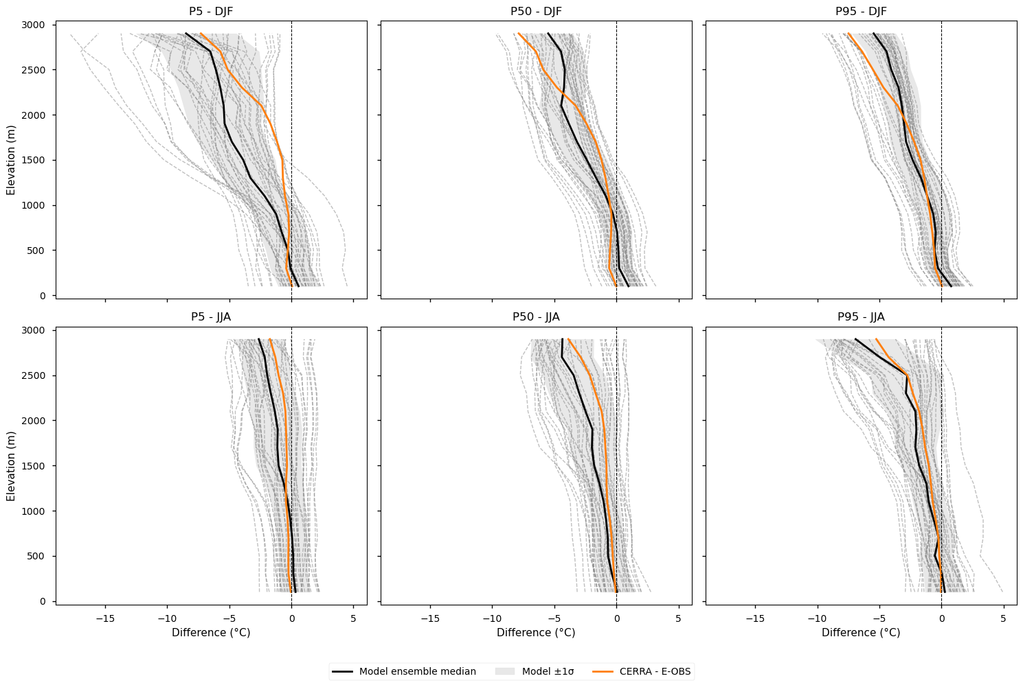
Fig 4. Elevation profiles of biases after applying lapse-rate correction. Differences compared to the E-OBS vertical profile are shown for each EURO-CORDEX model individually, the ensemble median, the spread (calculated as the standard deviation), and CERRA. Profiles are plotted separately for winter (DJF) and summer (JJA), and for the 5th, 50th, and 95th percentiles. The ensemble median is represented by a solid black line, while individual EURO-CORDEX models appear as grey dashed lines. The model spread, calculated as the standard deviation across models, is shown as a grey shaded area. CERRA is depicted in orange. No lapse-rate correction is applied in this case. An elevation correction using a uniform lapse rate is applied to each dataset prior to computing the differences, to account for altitude discrepancies between the model grids and the observational datasets (CERRA and E-OBS), relative to the model used as the target for regridding.
3.4. Elevation profiles of the impact of lapse-rate correction#
This section highlights the change introduced by the lapse-rate correction, showing the difference between corrected and uncorrected profiles for each dataset.
Show code cell source
plot_lapse_rate_impact(ds_models,ds_cerra,ds_eobs,
    ds_models_corrected,ds_cerra_corrected,
    ds_eobs_corrected,ds_orog_grid_out
)
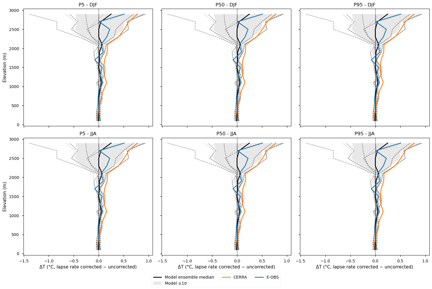
Fig 5. Elevation profiles of the impact of lapse-rate correction. This plot shows the difference between the corrected and uncorrected profiles for CERRA, E-OBS, individual EURO-CORDEX models, the ensemble median, and the spread. Results are disaggregated by season and percentile. The ensemble median is represented by a solid black line, while individual EURO-CORDEX models appear as grey dashed lines. The model spread, calculated as the standard deviation across models, is shown as a grey shaded area. CERRA is depicted in orange and E-OBS in blue.
3.5. Results summary#
Systematic biases are observed in the Regional Climate Models (RCMs) above 1000 to 1500 meters during winter across the 5th, 50th, and 95th percentiles.
The RCM bias patterns align with findings from [3], despite small differences in regions and reference periods.
Biases tend to increase in magnitude (becoming more negative with elevation), particularly for the 5th percentile in winter, where the ensemble median shows its largest negative value.
Even in summer, models generally exhibit negative biases at higher elevations, particularly for the 50th and 90th percentiles.
The greatest inter-model spread occurs for the 5th percentile in winter.
CERRA shows notably large cold biases relative to E-OBS; for the 50th and 95th percentiles in winter, it is even colder than the CMIP6 ensemble median above 2000–2500 meters.
The shape of the vertical bias profiles changes little when applying lapse-rate correction.
The lapse-rate correction has a stronger impact on E-OBS and especially on CERRA. The difference between corrected and uncorrected values grows with elevation but generally remains below 0.5 °C.
Typically, the correction results in positive differences, indicating that CERRA and E-OBS perceive higher elevations and ridges compared to the chosen target model grid for regridding.
3.6. Implications for the users#
Elevation-dependent biases in RCM outputs are systematic and significant above 1000–1500 m, particularly in winter, and affect all percentiles. Users working with climate data in mountainous regions should be aware that cold biases tend to intensify with elevation, especially for cold extremes (5th percentile), potentially influencing impact assessments and adaptation planning.
Bias magnitude and inter-model spread vary by season and percentile, with the greatest variability observed in winter cold tails (5th percentile). This highlights substantial uncertainty for extreme cold conditions at high elevations, which should be explicitly considered in risk and vulnerability evaluations.
CERRA exhibits strong cold differences when compared to E-OBS. This has two key implications: (1) caution is needed when using CERRA as a reference or input dataset for mountain climate analyses, and (2) despite its high resolution, the underlying model may not adequately represent complex high-altitude dynamics and processes.
A critical caveat lies in the inherent uncertainty and sparsity of observational data at high elevations, particularly in E-OBS. These limitations—stemming from sparse station coverage, complex topography, and measurement challenges—can cause some of the apparent model biases to actually reflect deficiencies in the reference data.
Interpolation accuracy generally declines with reduced station density, performs worse for spatially variable parameters (e.g. precipitation), and deteriorates further in areas of complex terrain such as mountainous regions [8]. Moreover, in some cases, E-OBS tends to report warmer values than national station datasets across the 5th, 50th, and 95th percentiles [3], and has been shown to overestimate temperatures in the distribution tails, even over moderately complex orography [9].
Lapse-rate correction slightly reduces biases by adjusting for elevation differences between datasets but does not fundamentally change the shape of vertical bias profiles. While useful for harmonising datasets, it is not a solution to the underlying model or observational issues driving the biases.
Where feasible, users may benefit from complementing gridded analyses with station-based evaluations corrected for elevation. While the CDS does not currently provide access to raw station-level data, external sources may be used
Altogether, the combination of systematic model biases, observational uncertainties, and limited high-elevation data availability underscores the need for caution when interpreting temperature extremes and climate signals in mountainous regions.
Bias-adjustment methods do not ensure that corrected future projections will more accurately reflect reality, as the underlying biases may change under evolving climate conditions [10].
ℹ️ If you want to know more#
Key resources#
Some key resources and further reading were linked throughout this assessment.
Regional climate models - CORDEX: https://cds.climate.copernicus.eu/datasets/projections-cordex-domains-single-levels?tab=overview
Gridded observation dataset for Europe, E-OBS: https://cds.climate.copernicus.eu/datasets/insitu-gridded-observations-europe?tab=overview
CERRA sub-daily regional reanalysis data for Europe on single levels from 1984 to present: https://cds.climate.copernicus.eu/datasets/reanalysis-cerra-single-levels?tab=overview
High-resolution global climate models: https://highresmip.org/
Mountain tourism meteorological and snow indicators for Europe from 1950 to 2100 derived from reanalysis and climate projections: https://cds.climate.copernicus.eu/datasets/sis-tourism-snow-indicators?tab=overview
Code libraries used:
C3S EQC custom functions,
c3s_eqc_automatic_quality_control, prepared by B-Open
References#
[1] Immerzeel, W.W., Lutz, A.F., Andrade, M. et al., 2020. Importance and vulnerability of the world’s water towers. Nature 577, 364–369. https://doi.org/10.1038/s41586-019-1822-y
[2] Rudisill, W., Rhoades, A., Xu, Z., and Feldman, D. R.,2024. Are Atmospheric Models Too Cold in the Mountains? The State of Science and Insights from the SAIL Field Campaign. Bull. Amer. Meteor. Soc., 105, E1237–E1264, https://doi.org/10.1175/BAMS-D-23-0082.1
[3] Matiu, M., Napoli, A., Kotlarski, S. et al., 2024. Elevation-dependent biases of raw and bias-adjusted EURO-CORDEX regional climate models in the European Alps. Clim Dyn 62, 9013–9030. https://doi.org/10.1007/s00382-024-07376-y
[4] Shrestha, S., Zaramella, M., Callegari, M., Greifeneder, F., Borga, M., 2023. Scale Dependence of Errors in Snow Water Equivalent Simulations Using ERA5 Reanalysis over Alpine Basins. Climate, 11, 154. https://doi.org/10.3390/cli11070154
[5] Haslinger, K., Holawe, F., and Blöschl, G., 2019. Spatial characteristics of precipitation shortfalls in the Greater Alpine Region—a data-based analysis from observations. Theor Appl Climatol 136, 717–731. https://doi.org/10.1007/s00704-018-2506-5
[6] Auer, I., Böhm, R., Jurkovic, A., Lipa, W., Orlik, A., Potzmann, R., Schöner, W., Ungersböck, M., Matulla, C., Briffa, K., Jones, P., Efthymiadis, D., Brunetti, M., Nanni, T., Maugeri, M., Mercalli, L., Mestre, O., Moisselin, J.-M., Begert, M., Müller-Westermeier, G., Kveton, V., Bochnicek, O., Stastny, P., Lapin, M., Szalai, S., Szentimrey, T., Cegnar, T., Dolinar, M., Gajic-Capka, M., Zaninovic, K., Majstorovic, Z. and Nieplova, E., 2007. HISTALP—historical instrumental climatological surface time series of the Greater Alpine Region. Int. J. Climatol., 27: 17-46. https://doi.org/10.1002/joc.1377
[7] Kotlarski, S., Szabó, P., Herrera S., et al., 2019. Observational uncertainty and regional climate model evaluation: A pan-European perspective. Int J Climatol. 39: 3730–3749. https://doi.org/10.1002/joc.5249
[8] Hofstra, N., Haylock, M., New, M., and Jones, P. D., 2009. Testing E-OBS European high-resolution gridded data set of daily precipitation and surface temperature, J. Geophys. Res., 114, D21101, doi:10.1029/2009JD011799.
[9] Kyselý, J., and Plavcová, E., 2010. A critical remark on the applicability of E-OBS European gridded temperature data set for validating control climate simulations, J. Geophys. Res., 115, D23118, doi:10.1029/2010JD014123.
[10] Schmith, T., Thejll, P., Berg, P., Boberg, F., Christensen, O. B., Christiansen, B., Christensen, J. H., Madsen, M. S., and Steger, C., 2021. Identifying robust bias adjustment methods for European extreme precipitation in a multi-model pseudo-reality setting, Hydrol. Earth Syst. Sci., 25, 273–290, https://doi.org/10.5194/hess-25-273-2021