Please note that this repository is used for development and review, so quality assessments should be considered work in progress until they are merged into the main branch

1.2.1. Consistency of carbon dioxide satellite observations for the evaluation of Earth system models.

Production date: 15-09-2025

Produced by: CNR

🌍 Use case: Using satellite observations for evaluating carbon dioxide growth rates and seasonal cycles provided by Earth System Models

❓ Quality assessment question

• Is the temporal consistency of the Level-3 Obs4MIPs merged dataset suitable for calculating changes in the annual growth rates of XCO₂ and the amplitude of the seasonal cycles?

The most important anthropogenic greenhouse gas is carbon dioxide (CO\(_2\)), with CO\(_2\) emissions contributing 66% of the total radiative forcing by long-lived greenhouse gases [1]. It is therefore important to monitor the long-term changes in atmospheric CO\(_2\) concentrations, to understand the sources and sinks of the atmospheric carbon content and to provide reliable projections of future CO\(_2\) concentrations under various scenarios.

Earth System Models (ESMs) are computer simulations that couple the physical climate (i.e. the atmosphere, the oceans and sea ice) with other components of the Earth, such as the land surface, vegetation, biogeochemistry (i.e. the carbon and nitrogen cycles), the cryosphere and, in some cases, human systems, in order to simulate how the entire Earth behaves now and in the future [2]. They are widely used, among other aims, to provide climate projections under different greenhouse gas and land use scenarios, to determine the contribution of human activities to observed changes or specific extreme events, to investigate biogeochemical cycles, and to inform mitigation pathways and climate risk analysis for policymakers.

In this assessment, we show how the column-averaged mixing ratios of CO\(_2\) (XCO\(_2\)) provided by the Obs4MIPs Level 3 data product of [3] can be used to evaluate the annual growth rates and seasonal cycles of CO\(_2\) provided by ESMs. The Obs4MIPs Level 3 data product results from integrating XCO₂ data from different combinations of satellite sensors and algorithms over time and space. Based on the results of references [4] and independent analyses, we investigate the impact of changes in the sampling characteristics of the Obs4MIPs dataset on the ability to use it to evaluate the capacity of ESMs to reproduce CO₂ seasonal cycle amplitudes and related trends/inter-annual variability, across its entire temporal coverage.

📢 Quality assessment statement

These are the key outcomes of this assessment

• The Obs4MIPs Lev3 merged dataset is suitable for assessing the capacity of Earth System Models to reproduce CO₂ growth rates and seasonal cycle variability, however the dataset features related to the spatial and temporal data coverage must be carefully considered (see points below).

• For annual aggregation, high-latitude regions (i.e.. latitudes higher than 60°N and 60°S) should not be considered due to non-uniform data coverage across the different seasons.

• The introduction of new satellite data (e.g., GOSAT in 2009 and OCO-2 in 2015) affects the data coverage at global scale with changing coverage of high latitude regions and oceans.

• The months characterised by changes in the contributing satellite data can show inconsistent CO₂ growth rates; however, this feature is averaged out when computing the annual growth.

• Changes in data coverage over the period covered by the Obs4MIPs Level 3 dataset affect the calculation of the seasonal cycle amplitude.

📋 Methodology

To assess if the temporal consistency of the Level-3 Obs4MIPs merged dataset from the Climate Data Store “Carbon dioxide data from 2002 to present derived from satellite observations” [3] is suitable for calculating changes in the annual growth rates of XCO\(_2\) and the amplitude of the seasonal cycles, we inspected a specific case study available from scientific literature [4] and we performed independent analyses. In particular, we analysed the changes of data coverage as a function of months and years, we calculated the monthly resolved CO\(_2\) annual growth rates and the annual seasonal cycles. To do that we used a methodology consistent with [4]. However, we perform our analyses over the period 2003 - 2022 by using the most recent version (4.5) of the Level-3 Obs4MIPs merged dataset [5]. This dataset is obtained by gridding the merged level-2 product generated with the ensemble median algorithm (XCO2_EMMA). EMMA combines several different XCO2 level-2 satellite data products: SCIAMACHY/Envisat (2003–2012), TANSO-FTS/GOSAT (2009–2022), OCO-2 (2014-2022), TANSO-FTS-2/GOSAT2 (2019-2022).

A previous study [4] evaluated emission-driven CMIP5 and CMIP6 simulations with satellite data of column-average CO\(_2\) mole fractions (XCO\(_2\)) by considering a earlier version of the Level-3 Obs4MIPs merged data product available by the Climate Data Store (Obs4MIPs, version 3) from 2003 to 2016. In particular, this previous study evaluated the agreement between CMIP5 and CMIP6 simulations with satellite data in depicting the annual growth rate of CO\(_2\) as well as the changes of seasonal cycle amplitude (SCA) with time.

More specifically, this notebook aims to:

• Generate global maps of monthly XCO\(_2\) data coverage, to show that the spatial coverage of data is not uniform across the different regions of the world for the different seasons.

• Generate global maps of XCO\(_2\) data coverage as a function of the different temporal periods covered by different satellite/sensors, i.e. SCIAMACHY/Envisat (2003–2012), TANSO-FTS/GOSAT (2009–2022), OCO-2 (2014-2022), TANSO-FTS-2/GOSAT2 (2019-2022).

• To calculate the global annual growth rates of XCO\(_2\) and the seasonal cycle amplitudes for the entire measurement period 2003-2022.

The analysis and results are organized in the following steps, which are detailed in the sections below:

1. Choose the data to use and set-up the code

• Import all relevant packages.

• Select the variable of interest

• Cache needed functions.

2. Retrieve data

• Define the data request to CDS.

3. Data analysis

This section presents several results for the XCO\(_2\) products, i.e.:

• The monthtly mean data coverage of XCO\(_2\) over the period 2003-2022.

• The mean data coverage of XCO\(_2\) over specific time periods characterised by the use of observations from different satellites.

• The calculation of the XCO\(_2\) growth rates and annual seasonal cycles by using an approach similar to that adopted by [4]. Specifically, we computed monthly resolved annual growth rates by subtracting the XCO\(_2\) value 6 months in the future from the one 6 months in the past. Then these monthly resolved growth rates are averaged to a yearly GR for a calendar year. We calculated the annual seasonal cycled of global XCO\(_2\) by detrending the monthly time series with the cumulative sum of monthly growth rates, using the annual mean growth rates as substitution for missing values where necessary. Finally, we normalised the time series of detrended monthly values by subtracting the average seasonal cycle over the whole period 2003 - 2022. Spatial averages are calculated by taking the arithmetic averages over all grid cells weighted by their area.

• Similarly to [4], we calculated of the annual seasonal cycle amplitudes (SCAs) as the peak-to-trough amplitude in a calendar year of the detrended time series.

📈 Analysis and results

1. Choose the data to use and set-up the code

Import all relevant packages

In this section, we import all the relevant packages needed for running the notebook and we define the style for plot appearance (“seaborn-v0_8-notebook”) as well as the style of hatches used in the maps.

Show code cell source

Hide code cell source

import calendar
import cartopy.crs as ccrs
import matplotlib.pyplot as plt
import matplotlib.dates as mdates
import numpy as np
import xarray as xr
import warnings #to suppress warning
import pandas as pd
from c3s_eqc_automatic_quality_control import diagnostics, download, plot, utils
from matplotlib.ticker import MaxNLocator, FuncFormatter

import os
os.environ["CDSAPI_RC"] = os.path.expanduser("~/putero_davide/.cdsapirc")

plt.style.use("seaborn-v0_8-notebook")
plt.rcParams["hatch.linewidth"] = 0.5

download.INVALIDATE_CACHE = True #Set True to invalidate the caching

warnings.filterwarnings("ignore") #To filter out warnings

Define the variable of interest

In this section, we define the parameters to be ingested by the code (that can be customized by the user), i.e.:

• the variable of interest.

Show code cell source

Hide code cell source

# Choose variable (xch4 or xco2)
variable = "xco2"
assert variable in [
    f"{prefix}{suffix}"
    for prefix in ("xch4", "xco2")
    for suffix in ("", "_nobs", "_stderr", "_stddev")
]

Cache needed functions

In this section, we cached a list of functions used in the analyses.

• The convert_units function rescales XCO\(_2\) mole fraction to parts per million (ppm).

• The compute_coverage function calculates the spatial fractional coverage of the available data and creates associated maps.

• The def area_weighted_series function calculates the spatial averages over all grid cells in a region. It uses spatial weighting to account for the latitudinal dependence of the grid size in the lon/lat grids.

• The compute_GR_and_seasonal funtion calculates the monthly resolved annual growth rates of XCO\(_2\) and the annual seasonal cycles.

Show code cell source

Hide code cell source

def get_da(
    ds, min_land_fraction, variable, year_start, year_stop, lon_slice, lat_slice
):
    da = ds[variable].sel(time=slice(str(year_start), str(year_stop)))
    da = utils.regionalise(da, lon_slice=lon_slice, lat_slice=lat_slice)
    if min_land_fraction is not None:
        return da.where(ds["land_fraction"] >= min_land_fraction)
    return da

def convert_units(da):
    if da.name.endswith("_nobs"):
        return da

    with xr.set_options(keep_attrs=True):
        if da.name.startswith("xch4") and da.attrs["units"] != "ppb":
            da *= 1.0e9
            da.attrs["units"] = "ppb"
        elif da.name.startswith("xco2") and da.attrs["units"] != "ppm":
            da *= 1.0e6
            da.attrs["units"] = "ppm"
    return da

def compute_coverage(da, missing_values=1.0e20, dim="time"):
    return (da != missing_values).sum(dim) / da.sizes[dim]

def area_weighted_series(xda, weights2d):
    # numerator: sum over lat,lon of x * weight (ignore NaNs in x)
    num = (xda * weights2d).where(~np.isnan(xda)).sum(dim=("latitude", "longitude"))
    den = weights2d.where(~np.isnan(xda)).sum(dim=("latitude", "longitude"))
    # avoid division by zero
    ts = (num / den)
    return ts.to_series()

def compute_GR_and_seasonal(series):
    """
    series: pandas.Series indexed by Timestamp (monthly)
    returns: monthly_GR (ppm/yr, pandas.Series), seasonal (ppm, pandas.Series)
    """
    # convert to xarray DataArray with time coords
    s_xr = xr.DataArray(series.values, coords={"time": series.index}, dims=("time",))
    # compute GR: GR(m) = x(t+6) - x(t-6)
    xco2_future = s_xr.shift(time=-6)
    xco2_past   = s_xr.shift(time=+6)
    monthly_GR = (xco2_future - xco2_past).to_series()

    # annual mean GR (used to substitute missing monthly GR)
    yearly_GR = monthly_GR.groupby(monthly_GR.index.year).mean()

    # fill monthly GR missing with annual mean where possible
    monthly_GR_filled = monthly_GR.copy()
    for year, val in yearly_GR.items():
        if np.isfinite(val):
            idx = monthly_GR_filled.index.year == year
            monthly_GR_filled.loc[idx] = monthly_GR_filled.loc[idx].fillna(val)

    # monthly increment (ppm/month) from yearly GR
    monthly_trend = monthly_GR.copy()
    for year, val in yearly_GR.items():
        idx = monthly_trend.index.year == year
        if np.isfinite(val):
            monthly_trend.loc[idx] = val / 12.0
        else:
            monthly_trend.loc[idx] = np.nan

    # cumulative trend (ppm)
    trend = monthly_trend.cumsum()

    # seasonal cycle: xco2 - cumulative trend ; center to zero mean
    seasonal = series - trend
    seasonal = seasonal - seasonal.mean()

    return monthly_GR, seasonal    

2. Retrieve data

2.1 Obs4MIPs

In this section, we define the data request to CDS (data product Obs4MIPs, Level 3, version 4.5, XCO\(_2\)) and download the full dataset.

Show code cell source

Hide code cell source

request = (
    "satellite-carbon-dioxide" if variable.startswith("xco2") else "satellite-methane",
    {
        "processing_level": ["level_3"],
        "variable": variable.split("_")[0],
        "sensor_and_algorithm": "merged_obs4mips",
        "version": ["4_5"],
        "format": ["zip"],
    },
)

3. Data analysis

Global maps of monthly XCO\(_2\) data coverage

In this section, we calculate and plot the mean monthly fractional coverage of data over the period 2003 - 2022. In agreement with the results by [4], the number of available observations depends significantly on the location with low data coverage values over locations typically affected by high cloud coverage (like tropics) and low Sun elevation (like high latitude in winter months). Coverage over ocean is sparse as ocean retrievals are included from GOSAT, OCO-2 and GOSAT2 Sun-glint mode observations. [4] demonstrated that taking into account this sampling coverage feature is essential for a proper comparison with outputs from ESMs.

Show code cell source

Hide code cell source

ds = download.download_and_transform(*request)
da = ds["xco2"].groupby("time.month").map(compute_coverage)
da["month"] = [calendar.month_name[month] for month in da["month"].values]
da.attrs = {"long_name": "XCO$_2$ Data Coverage"}
facet = plot.projected_map(
    da,
    plot_func="contourf",
    col="month",
    col_wrap=3,
    cmap="Greens",
    cbar_kwargs={"orientation": "horizontal"},
    vmin=0,
    vmax=1,
    levels=11,
)

  0%|          | 0/1 [00:00<?, ?it/s]2025-09-15 16:03:44,233 INFO [2025-09-03T00:00:00] To improve our C3S service, we need to hear from you! Please complete this very short [survey](https://confluence.ecmwf.int/x/E7uBEQ/). Thank you.
2025-09-15 16:03:44,234 INFO [2024-09-26T00:00:00] Watch our [Forum](https://forum.ecmwf.int/) for Announcements, news and other discussed topics.
2025-09-15 16:03:44,451 INFO [2025-09-03T00:00:00] To improve our C3S service, we need to hear from you! Please complete this very short [survey](https://confluence.ecmwf.int/x/E7uBEQ/). Thank you.
2025-09-15 16:03:44,452 INFO [2024-09-26T00:00:00] Watch our [Forum](https://forum.ecmwf.int/) for Announcements, news and other discussed topics.
2025-09-15 16:03:44,628 INFO Request ID is 40d292e5-b4ff-4bb3-90df-b1b024ce7034
2025-09-15 16:03:44,706 INFO status has been updated to accepted
2025-09-15 16:03:58,197 INFO status has been updated to running
2025-09-15 16:04:34,397 INFO status has been updated to successful

a87f027c6b4189cffe45c5c8be80fcbb.zip:   0%|          | 0.00/57.0M [00:00<?, ?B/s]
a87f027c6b4189cffe45c5c8be80fcbb.zip:   2%|▏         | 1.00M/57.0M [00:00<00:42, 1.37MB/s]
a87f027c6b4189cffe45c5c8be80fcbb.zip:   5%|▌         | 3.00M/57.0M [00:03<01:03, 886kB/s] 
a87f027c6b4189cffe45c5c8be80fcbb.zip:   7%|▋         | 4.00M/57.0M [00:06<01:33, 597kB/s]
a87f027c6b4189cffe45c5c8be80fcbb.zip:   9%|▉         | 5.00M/57.0M [00:07<01:18, 699kB/s]
a87f027c6b4189cffe45c5c8be80fcbb.zip:  11%|█         | 6.00M/57.0M [00:07<00:55, 965kB/s]
a87f027c6b4189cffe45c5c8be80fcbb.zip:  12%|█▏        | 7.00M/57.0M [00:07<00:40, 1.29MB/s]
a87f027c6b4189cffe45c5c8be80fcbb.zip:  14%|█▍        | 8.00M/57.0M [00:07<00:30, 1.70MB/s]
a87f027c6b4189cffe45c5c8be80fcbb.zip:  16%|█▌        | 9.00M/57.0M [00:08<00:22, 2.22MB/s]
a87f027c6b4189cffe45c5c8be80fcbb.zip:  18%|█▊        | 10.0M/57.0M [00:08<00:17, 2.84MB/s]
a87f027c6b4189cffe45c5c8be80fcbb.zip:  19%|█▉        | 11.0M/57.0M [00:08<00:13, 3.50MB/s]
a87f027c6b4189cffe45c5c8be80fcbb.zip:  23%|██▎       | 13.0M/57.0M [00:08<00:09, 4.88MB/s]
a87f027c6b4189cffe45c5c8be80fcbb.zip:  25%|██▍       | 14.0M/57.0M [00:08<00:08, 5.57MB/s]
a87f027c6b4189cffe45c5c8be80fcbb.zip:  26%|██▋       | 15.0M/57.0M [00:08<00:07, 6.20MB/s]
a87f027c6b4189cffe45c5c8be80fcbb.zip:  30%|██▉       | 17.0M/57.0M [00:08<00:05, 7.65MB/s]
a87f027c6b4189cffe45c5c8be80fcbb.zip:  33%|███▎      | 19.0M/57.0M [00:09<00:04, 8.94MB/s]
a87f027c6b4189cffe45c5c8be80fcbb.zip:  37%|███▋      | 21.0M/57.0M [00:09<00:03, 9.80MB/s]
a87f027c6b4189cffe45c5c8be80fcbb.zip:  40%|████      | 23.0M/57.0M [00:09<00:03, 10.5MB/s]
a87f027c6b4189cffe45c5c8be80fcbb.zip:  44%|████▍     | 25.0M/57.0M [00:09<00:02, 11.2MB/s]
a87f027c6b4189cffe45c5c8be80fcbb.zip:  47%|████▋     | 27.0M/57.0M [00:09<00:02, 11.9MB/s]
a87f027c6b4189cffe45c5c8be80fcbb.zip:  51%|█████     | 29.0M/57.0M [00:09<00:02, 12.5MB/s]
a87f027c6b4189cffe45c5c8be80fcbb.zip:  54%|█████▍    | 31.0M/57.0M [00:10<00:02, 12.9MB/s]
a87f027c6b4189cffe45c5c8be80fcbb.zip:  58%|█████▊    | 33.0M/57.0M [00:10<00:01, 14.2MB/s]
a87f027c6b4189cffe45c5c8be80fcbb.zip:  61%|██████▏   | 35.0M/57.0M [00:10<00:01, 13.8MB/s]
a87f027c6b4189cffe45c5c8be80fcbb.zip:  65%|██████▍   | 37.0M/57.0M [00:10<00:01, 14.5MB/s]
a87f027c6b4189cffe45c5c8be80fcbb.zip:  68%|██████▊   | 39.0M/57.0M [00:10<00:01, 14.2MB/s]
a87f027c6b4189cffe45c5c8be80fcbb.zip:  72%|███████▏  | 41.0M/57.0M [00:10<00:01, 14.9MB/s]
a87f027c6b4189cffe45c5c8be80fcbb.zip:  75%|███████▌  | 43.0M/57.0M [00:10<00:00, 15.5MB/s]
a87f027c6b4189cffe45c5c8be80fcbb.zip:  79%|███████▉  | 45.0M/57.0M [00:10<00:00, 15.6MB/s]
a87f027c6b4189cffe45c5c8be80fcbb.zip:  82%|████████▏ | 47.0M/57.0M [00:11<00:00, 16.6MB/s]
a87f027c6b4189cffe45c5c8be80fcbb.zip:  86%|████████▌ | 49.0M/57.0M [00:11<00:00, 16.6MB/s]
a87f027c6b4189cffe45c5c8be80fcbb.zip:  91%|█████████ | 52.0M/57.0M [00:11<00:00, 17.4MB/s]
a87f027c6b4189cffe45c5c8be80fcbb.zip:  95%|█████████▍| 54.0M/57.0M [00:12<00:00, 5.61MB/s]
a87f027c6b4189cffe45c5c8be80fcbb.zip:  98%|█████████▊| 56.0M/57.0M [00:12<00:00, 6.96MB/s]
                                                                                          
  0%|          | 0/1 [00:00<?, ?it/s]
100%|██████████| 1/1 [01:08<00:00, 68.73s/it]

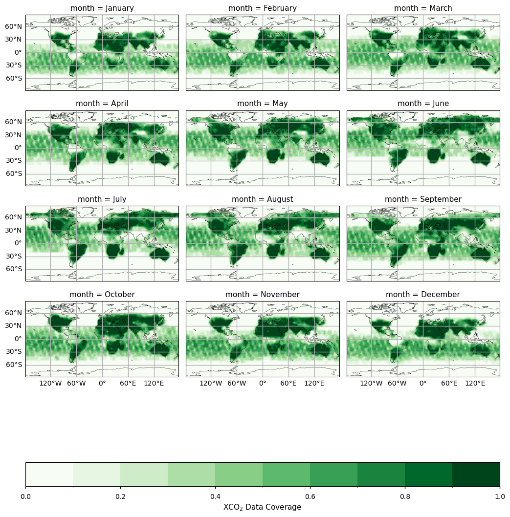
The figure shows the monthly fractional XCO\(_2\) data coverage from 2003 to 2022 derived from the XCO2_OBS4MIPS dataset (version 4.5).

Global maps of XCO\(_2\) data coverage for different periods

In this section, to assess the temporal consistency of spatial data coverage over the whole period covered by the Level-3 Obs4MIPs merged dataset, we calculate and plot the mean fractional coverage of CO\(_2\) data for time periods characterised by the contribution of different satellite observations: i.e., 2003 - 2008 (only SCIAMACHY observations), 2009 - 2011 (combination of SCIAMACHY and GOSAT), 2012 - 2014 (GOSAT), 2015 - 2018 (combination of GOSAT and OCO-2), 2019 -2022 (combination of GOSAT, OCO-2 and GOSAT2). A comprehensive analysis of the number of soundings contained within the EMMA database on a monthly basis, along with the comparative contribution of each individual Level 2 algorithm to the EMMA database, can be found in [6].

Besides not including data over oceans, with respect to subsequent periods in which GOSAT measurements were used (2009 - 2011 and 2012 - 2014), for the period 2003 - 2008 more data are available for regions higher than 50°N as well as over tropical regions in South America and Africa. The introduction of OCO-2 and GOSAT2 observations (2015–2018 and 2019–2022, respectively) resulted in an increase of the data coverage over Europe and the oceans. A substantial proportion of these regions exhibited data coverage levels exceeding 0.5, with the data extending to higher latitudes.

Show code cell source

Hide code cell source

# To define temporal coverage
bins   = pd.to_datetime(["2003-01-01","2009-01-01","2012-01-01","2015-01-01","2019-01-01","2023-01-01"])
labels = ["SCHIAMACHY (2003-2008)", "SCHIAMACHY+GOSAT (2009-2011)", "GOSAT (2012-2014)", "GOSAT+OCO-2  (2015-2018)", "GOSAT+OCO-2+GOSAT2 (2019-2012)"]

interval_coord = pd.cut(ds["time"].to_index(), bins=bins, labels=labels, right=False)
ds_1 = ds.assign_coords(interval=("time", interval_coord))

# To categorise data coverage as a function of time periods
da = ds_1["xco2"].groupby("interval").map(compute_coverage)
da.attrs = {"long_name": "XCO$_2$ Data Coverage"}

# Plotting
facet = plot.projected_map(
    da,
    plot_func="contourf",
    col="interval",
    col_wrap=1,
    cmap="Greens",
    cbar_kwargs={"orientation": "horizontal"},
    vmin=0,
    vmax=1,
    levels=11,
    # add custom labels
    col_labels=labels
)

facet.set_titles("{value}") 

# Add hatched pattern where coverage > 0.5
for ax, (_, subda) in zip(facet.axes.flatten(), da.groupby("interval")):
    # convert to 2D array (lat, lon)
    sub2d = subda.squeeze()
    # mask values <=0.5
    hatched = sub2d.where(sub2d > 0.5)
    ax.contourf(
        hatched["longitude"],
        hatched["latitude"],
        hatched,
        levels=[0.5, 1],
        hatches=["///"],
        colors="none",
        alpha=0
    )
    
# Adjust layout and move colorbar below all maps
facet.fig.tight_layout()
facet.fig.subplots_adjust(bottom=0.1, top=0.78, hspace=0.1)
facet.cbar.ax.set_position([0.25, 0.03, 0.5, 0.03])

plt.show()

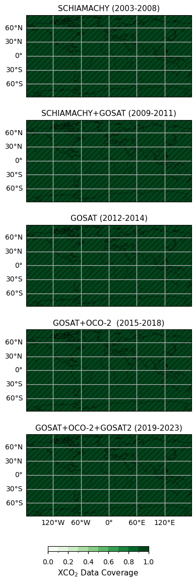
The figure shows the monthly fractional XCO\(_2\) data coverage for different time periods characterised by the use of different satellites/sensors to obtain obervations. The hatched areas denote regions with data coverage higher than 0.5

Calculation of growth rate and seasonal cycles

In this section, we calculate and report the time series of monthly global CO₂ values, the resolved annual growth rate, and the seasonal cycles. Over the period 2003–2014, our average growth rate of 2.02 ppm/year (with a standard deviation of 0.49 ppm/year) is in very good agreement with the values provided in [4]. The calculated seasonal cycles also completely agree with those calculated in [4], which report a clear change in shape and amplitude when GOSAT observations began contributing to the calculation of global CO₂ in 2009. The low growth rate observed in 2009 is due to the introduction of GOSAT data, which altered the shape of the seasonal cycle. When considering only land-based data (orange lines), the low growth rate in 2009 disappears, and the seasonal cycles appear more consistent throughout the measurement period with an higher amplitude due to the higher carbon fluxes occurring over land regions than over oceans. This clearly shows that any changes to the sampling features that occur during the period covered by the dataset must be taken into account, particularly when evaluating uniform, gap-free datasets such as those provided by ESMs. The high growth rate values observed in 2010, 2012, 2016 and 2019 are consistent with those reported by the in situ global network coordinated by [1], and are related to El Niño conditions which favour net carbon emissions into the atmosphere on a global scale.

Show code cell source

Hide code cell source

# -------------------------------------------------------
# Load dataset and basic preprocess
# -------------------------------------------------------
#ds = download.download_and_transform(*request)

# Replace missing value 1.0e20 with NaN
ds["xco2"] = ds["xco2"].where(ds["xco2"] != 1.0e20)

# Convert xco2 to ppm
ds["xco2"] = ds["xco2"] * 1e6

# -------------------------------------------------------
# Prepare area weights (cos(lat)) as 2D DataArray (lat, lon)
# -------------------------------------------------------
lat_rad = np.deg2rad(ds["latitude"].values)
lat_weights_1d = np.cos(lat_rad)
weights_lat = xr.DataArray(lat_weights_1d, coords={"latitude": ds["latitude"]}, dims=("latitude",))
ones_2d = xr.ones_like(ds["xco2"].isel(time=0))  # shape (latitude, longitude)
weights_2d_raw = weights_lat * ones_2d            # broadcast to (latitude, longitude)

# -------------------------------------------------------
# land mask: keep only cells with land_fraction > 0.5
# -------------------------------------------------------
land_mask = ds["land_fraction"] > 0.5  # dims (latitude, longitude)
# weights masked
weights_2d_masked = weights_2d_raw * land_mask

# -------------------------------------------------------
# Compute series for both cases: all gridcells and masked (land_fraction>0.5)
# -------------------------------------------------------
x_all = ds["xco2"]                     # all points
x_masked = ds["xco2"].where(land_mask)  # masked xco2 (NaN outside mask)

# area-weighted global series
global_all_series = area_weighted_series(x_all, weights_2d_raw)
global_masked_series = area_weighted_series(x_masked, weights_2d_masked)

# compute monthly GR and seasonal cycle for both
monthly_GR_all, seasonal_all = compute_GR_and_seasonal(global_all_series)
monthly_GR_masked, seasonal_masked = compute_GR_and_seasonal(global_masked_series)

# -------------------------------------------------------
# Quick diagnostics (optional prints)
# -------------------------------------------------------
#print("Global (all) series length:", len(global_all_series.dropna()))
#print("Global (masked) series length:", len(global_masked_series.dropna()))
#print("Fraction positive GR (all):", (monthly_GR_all.dropna() > 0).mean())
#print("Fraction positive GR (masked):", (monthly_GR_masked.dropna() > 0).mean())

# -------------------------------------------------------
# Plotting: three vertical plots with both lines
# -------------------------------------------------------
cmap = plt.get_cmap("tab10")
color_all = cmap(0)
color_mask = cmap(1)

fig, axes = plt.subplots(nrows=3, ncols=1, figsize=(14, 12), sharex=True, constrained_layout=False)

# (1) Global monthly mean XCO2
axes[0].plot(global_all_series.index, global_all_series.values, label="All data", color=color_all, linestyle="-", linewidth=1.5)
axes[0].plot(global_masked_series.index, global_masked_series.values, label="Land_fraction > 0.5", color=color_mask, linestyle="--", linewidth=1.5)
axes[0].set_ylabel("xco2 (ppm)", fontsize=12)
axes[0].set_title("Global Monthly Mean XCO₂", fontsize=14)
axes[0].legend(loc="best")

# (2) Monthly Growth Rate (ppm/yr)
axes[1].plot(monthly_GR_all.index, monthly_GR_all.values, label="All data", color=color_all, linestyle="-", linewidth=1.5)
axes[1].plot(monthly_GR_masked.index, monthly_GR_masked.values, label="Land_fraction > 0.5", color=color_mask, linestyle="--", linewidth=1.5)
axes[1].set_ylabel("GR (ppm/yr)", fontsize=12)
axes[1].set_title("Monthly Growth Rate (GR)", fontsize=14)
axes[1].legend(loc="best")

# add stats box for both series (means and stds)
mean_all = monthly_GR_all.mean()
std_all = monthly_GR_all.std()
mean_mask = monthly_GR_masked.mean()
std_mask = monthly_GR_masked.std()
textstr = (
    f"All: mean={mean_all:.2f}, std={std_all:.2f}\n"
    f"Mask: mean={mean_mask:.2f}, std={std_mask:.2f}"
)
axes[1].text(0.55, 0.15, textstr, transform=axes[1].transAxes, fontsize=10,
             verticalalignment='top', bbox=dict(boxstyle='round', facecolor='white', alpha=0.6))

# (3) Seasonal Cycle (detrended)
axes[2].plot(seasonal_all.index, seasonal_all.values, label="All data", color=color_all, linestyle="-", linewidth=1.5)
axes[2].plot(seasonal_masked.index, seasonal_masked.values, label="Land_fraction > 0.5", color=color_mask, linestyle="--", linewidth=1.5)
axes[2].set_ylabel("Seasonal cycle (ppm)", fontsize=12)
axes[2].set_xlabel("Year", fontsize=12)
axes[2].set_title("Detrended Seasonal Cycle", fontsize=14)
axes[2].legend(loc="best")

# center y-axis of seasonal cycle around zero (symmetric limits) using both series combined
combined = np.concatenate([seasonal_all.dropna().values, seasonal_masked.dropna().values])
if combined.size > 0:
    ymax = np.nanmax(np.abs(combined))
    axes[2].set_ylim(-ymax, ymax)
    axes[2].axhline(0, linewidth=1, color="k", alpha=0.5)

# -------------------------
# Format x-axis to show integer years
# -------------------------
axes[2].xaxis.set_major_locator(mdates.YearLocator(base=1))   # one tick per year
axes[2].xaxis.set_major_formatter(mdates.DateFormatter('%Y'))
plt.setp(axes[2].get_xticklabels(), rotation=45, ha="right")

fig.tight_layout()
plt.show()

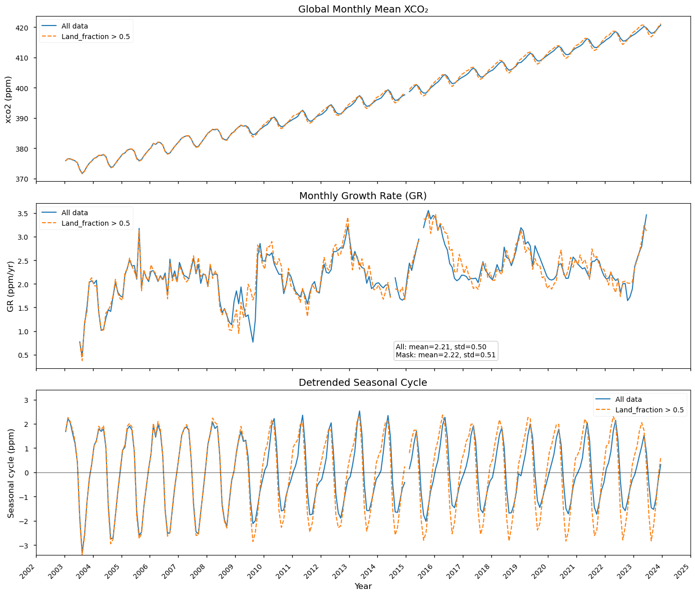
The figure shows the global time series of monthly XCO\(_2\) mean values (upper panel), monthly resolved annual growth rate (middle panel) and detrended seasonal cycles (bottom panel) from 2003 to 2022. Blue lines indicate results for the whole dataset, orange lines indicate results for land-masked data.

Calculation of the Seasonal Cycle Amplitude (SCA)

In this section, we show the time series of the annual global SCA calculated for the XCO\(_2\) variables for the whole dataset (blue) as well as for the land data (orange). Overall, the global SCA shows a decreasing trend over the period 2003 - 2022, however it should be pointed out that discontinuities exist at the time when new satellite observations were added to retrieve XCO\(_2\): especially GOSAT in 2009 and OCO-2 in 2015. When the land data only are considered, the negative tendency diappeared from 2008 onward in agreement with the ESM simulations reported by [4]. The high SCA amplitude observed in 2003 can be partially attributed to the relatively high global bias of the SCIAMACHY data product in the first half of the year created by the BESD (Bremen Optimal Estimation DOAS) algorithm (see Figure 5 in [6]).

Show code cell source

Hide code cell source

# ---------------------------------------------------------------------
# Compute the SCA (peak-to-trough amplitude in each year, min 7 months of data)
# ---------------------------------------------------------------------
sca_list = []
dt_df = seasonal_all

for year, sub in dt_df.groupby(dt_df.index.year):
    valid = sub.dropna()
    if len(valid) >= 7:
        sca_list.append({"year":year, "SCA": valid.max() - valid.min()})
    else:
        sca_list.append({"year":year, "SCA": np.nan})

sca_all = pd.DataFrame(sca_list).set_index("year")

sca_list_masked = []
dt_df = seasonal_masked

for year, sub in dt_df.groupby(dt_df.index.year):
    valid = sub.dropna()
    if len(valid) >= 7:
        sca_list_masked.append({"year":year, "SCA": valid.max() - valid.min()})
    else:
        sca_list_masked.append({"year":year, "SCA": np.nan})

sca_masked = pd.DataFrame(sca_list_masked).set_index("year")

#------------------------------------------------------------------------------
# Plotting
#------------------------------------------------------------------------------
colors = plt.get_cmap("tab10")

fig, axes = plt.subplots(
    nrows=1,
    figsize=(10, 5),
    sharex=True,
    constrained_layout=True
)

# (1) SCA plot
axes.plot(sca_all.index, sca_all.values, color=color_all, label="All data")
axes.plot(sca_all.index, sca_all.values, 'D', color=color_all)
axes.plot(sca_masked.index, sca_masked.values, color=color_mask, label="Land fraction > 0.5")
axes.plot(sca_masked.index, sca_masked.values, 'P', color=color_mask)
axes.set_ylabel("Seasonal Cycle Amplitude (ppm)", fontsize=14)
axes.set_xlabel("Years", fontsize=14)
axes.set_xlim(2003, 2023)
axes.set_ylim(3, 6)
axes.xaxis.set_major_locator(MaxNLocator(integer=True))
axes.set_title("Global Monthly Mean XCO₂", fontsize=14)
axes.legend();

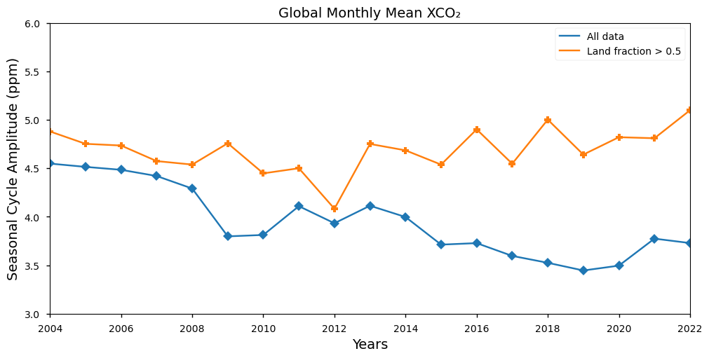
The figure shows the annual time series of SCA from 2003 to 2022 for the whole dataset (blue) and for land-masked data (orange).

ℹ️ If you want to know more

Key resources

The CDS catalogue entries for the data used were:

• Carbon dioxide data from 2002 to present derived from satellite observations: https://cds.climate.copernicus.eu/datasets/satellite-carbon-dioxide?tab=overview

Code libraries used:

• C3S EQC custom functions, c3s_eqc_automatic_quality_control, prepared by B-Open

Users interested in accessing official C3S products about long term trends of greenhouse gases from satellite observations are encouraged to access specifically designed Copernicus resources like the European State of Climate or the Global Climate Highlights.

Users interested in the investigation of CO\(_2\) fluxes can consider to use specifically designed Copernicus resources like CAMS global inversion-optimised greenhouse gas fluxes and concentrations.

References

[1] World Meteorological Organization. (2024). WMO Greenhouse Gas Bulletin, 20, ISSN 2078-0796.

[2] Eyring, V., Bony, S., Meehl, G. A., Senior, C. A., Stevens, B., Stouffer, R. J., and Taylor, K. E. (2016). Overview of the Coupled Model Intercomparison Project Phase 6 (CMIP6) experimental design and organization, Geoscience Model Development, 9, 1937–1958.

[3] Copernicus Climate Change Service, Climate Data Store. (2018). Carbon dioxide data from 2002 to present derived from satellite observations. Copernicus Climate Change Service (C3S) Climate Data Store (CDS) (Accessed on 23-Aug-2025).

[4] Gier, B. K., Buchwitz, M., Reuter, M., Cox, P. M., Friedlingstein, P., and Eyring, V. (2020). Spatially resolved evaluation of Earth system models with satellite column-averaged CO2, Biogeosciences, 17, 6115–6144.

[5] Buchwitz, M. (2024). Product User Guide and Specification (PUGS) – Main document for Greenhouse Gas (GHG: CO\(_2\) & CH\(_4\)) data set CDR7 (01.2003-12.2022), C3S project 2021/C3S2_312a_Lot2_DLR/SC1, v7.3.

[6] Reuter, M., and Buchwitz, M. (2024). Algorithm Theoretical Basis Document (ATBD) – ANNEX D for products XCO2_EMMA, XCH4_EMMA, XCO2_OBS4MIPS, XCH4_OBS4MIPS (v4.5, CDR7, 2003-2022), C3S project 2021/C3S2_312a_Lot2_DLR/SC1, v7.1b.