CMIP6 biases in SPEI6 drought simulations over the Mediterranean region

5.1.1. CMIP6 biases in SPEI6 drought simulations over the Mediterranean region#

Production date: 20-09-2025

Produced by: CMCC foundation - Euro-Mediterranean Center on Climate Change. Albert Martinez Boti and Lorenzo Sangelantoni.

🌍 Use case: Investigating drought biases to inform water management#

❓ Quality assessment question#

How well do CMIP6 models simulate drought compared to signals derived from ERA5?

The Standardized Precipitation-Evapotranspiration Index (SPEI) [1] is a widely used drought indicator that integrates precipitation and potential evapotranspiration, providing a more complete measure of water deficits than precipitation alone. Its multiscalar formulation allows the evaluation of different types of drought [2], from short-term agricultural or soil moisture deficits to long-term hydrological or ecological events. Being standardized, SPEI is dimensionless, facilitating comparisons across regions and climates. By capturing variations in frequency, duration, and severity, it effectively reflects the complex nature of drought, making it a robust and physically meaningful proxy for drought assessment in the context of climate change [3].

Understanding SPEI is particularly relevant for the water management sector. By capturing multiple types of drought SPEI serves as a versatile indicator for various users. Climate projections using SPEI enable planners to anticipate future water deficits, guide allocation, and design effective strategies for reservoir management, irrigation, and drought preparedness, helping to reduce socio-economic and ecological impacts [4][5].

This assessment evaluates SPEI6 (six-month accumulation) across the full ensemble of CMIP6 models available through the Copernicus Climate Data Store (CDS). Model outputs are compared against SPEI6 derived from ERA5 reanalysis, which serves as the reference product. The standard reference period is 1971–2010. We specifically evaluate whether changes in the 1991–2020 period relative to the 1961–1990 baseline are accurately represented by CMIP6 models and the trend acroos the whole 1961-2020 period for the Mediterranean domain.

📢 Quality assessment statement#

These are the key outcomes of this assessment

CMIP6 ensemble median captures the general intensification of drought over the Mediterranean seen in ERA5, though the magnitude of the change is underestimated, particularly over eastern Spain, southern France, and much of Turkey.
Individual models do not reproduce the same spatial pattern, highlighting the importance of using large ensembles rather than relying on a single model for planning purposes.
Despite inherent biases, the considered subset of CMIP6 models provides a foundation for understanding the evolution of past drought conditions. These results support the use of SPEI to anticipate water deficits and guide drought preparedness, increasing confidence (though not ensuring accuracy) when assessing future trends.
Regions with high inter-model spread, such as North Africa, Turkey, and the eastern Mediterranean, may be associated with future higher uncertainty, suggesting that adaptation strategies in these areas should consider a wider range of possible futures.

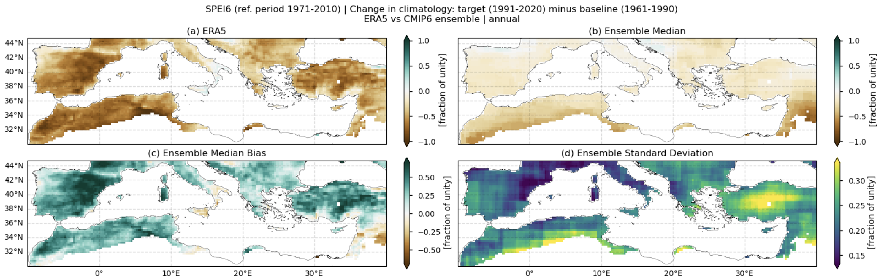
Visual abstract — Fig. 5.1.1.1 Spatial patterns of SPEI6 change over the Mediterranean region. Panels show (a) ERA5 reference, (b) CMIP6 ensemble median (median of the selected subset of models at each grid cell), (c) ensemble median bias relative to ERA5, and (d) ensemble spread (standard deviation across the selected models). SPEI6 is standardised over the reference period 1971–2010. SPEI6 change is calculated at each grid point as the difference between the monthly climatologies of the target period (1991–2020) and the baseline period (1961–1990), and then averaged to obtain the annual mean.#

📋 Methodology#

The Standardized Precipitation-Evapotranspiration Index accumulated to six months (SPEI6) has been calculated for this assessment — through the use of xclim — as a proxy to evaluate drought conditions for a subset of CMIP6 models, which are evaluated against SPEI6 derived from ERA5 reanalysis. The study covers the Mediterranean domain, following IPCC-AR6 regional definitions [6], and results include spatial maps of SPEI6 changes for ERA5, CMIP6, and the biases of these changes. Additionally, time series showing the temporal evolution of drought across the domain are calculated, comparing trends from the models with ERA5 over the historical period considered within this assessment (1961–2020).

Potential evapotranspiration (PET) is calculated with the Hargreaves method [7], which requires only maximum and minimum temperatures (and optionally mean temperature), providing a computationally efficient yet robust estimate (e.g., [8],). The accumulated series of precipitation minus PET is standardized for the reference period defined by the C3S Atlas (1971–2010).

Five key concepts are defined:

Reference period: The period used to standardize SPEI values, here 1971–2010, following the C3S Atlas.
Baseline period: The period against which changes are calculated, here 1961–1990.
Target period: The period for which changes are evaluated, here 1991–2020.
Historical period: The entire period considered in this assessment, here 1961–2020.
Change assessment: Differences in SPEI6 between the target period and the baseline, representing anomalies in drought conditions.

The analysis and results follow the next outline:

1. Parameters, requests and functions definition

1.1. Import packages
1.2. Define Parameters
1.3. Define models
1.4. Define ERA5 request
1.5. Define model requests
1.6. Functions to cache

2. Downloading and processing

2.1. Download and transform ERA5
2.2. Download and transform models
2.3. Apply land-sea mask and change some attributes

3. Plot and describe results

3.1. Define plotting functions
3.2. Plot ensemble maps
3.3. Plot model maps
3.4. Plot bias maps
3.5. Timeseries
3.6. Results summary
3.7. Implications for the users

📈 Analysis and results#

1. Parameters, requests and functions definition#

1.1. Import packages#

1.2. Define Parameters#

In the “Define Parameters” section, various customisable options for the notebook are specified:

The historical period can be adjusted by modifying historical_slice; the default range is 1961-2020.
The reference period can be adjusted by modifying reference_slice; the default range is 1971–2010, following the C3S Atlas.
The baseline period can be adjusted by modifying baseline_slice; the default range is 1961-1990.
The target period can be adjusted by modifying target_slice; the default range is 1991-2020.
The interpolation_method parameter allows selecting the interpolation method when regridding is performed.
collection_id is not customisable for this assessment and is set to ‘CMIP6’. Expert users can use this notebook as a guide to create similar analyses for other model sets (such as CORDEX).
The area parameter specifies the geographical domain of interest. By default, the Mediterranean domain is used, following IPCC-AR6 regional definitions [6]
The time_agg allows selecting the time aggregation for the analysis. Options include: annual, DJF, MAM, JJA, SON, Jan, Feb, Mar, Apr, May, Jun, Jul, Aug, Sep, Oct, Nov, Dec.
SPEI accumulation window (window): Defines the accumulation period in months for the SPEI calculation. Common options include 3, 6, or 12 months, depending on whether short-term or long-term droughts are of interest. In this assessment, a six-month accumulation is used.
The chunks selection allows the user to define if dividing into chunks when downloading the data on their local machine. Although it does not significantly affect the analysis, it is recommended to keep the default value for optimal performance.

1.3. Define models#

The following climate analyses are performed using CMIP6 models that provide both the historical and SSP5-8.5 experiments, as well as maximum, minimum and mean temperatures and precipitation, within the Climate Data Store (CDS).

1.4. Define ERA5 request#

Within this notebook, ERA5 serves as the reference product. In this section, we set the required parameters for the cds-api data-request of ERA5.

1.5. Define model requests#

In this section we set the required parameters for the cds-api data-request.

1.6. Functions to cache#

In this section, functions that will be executed in the caching phase are defined. Caching is the process of storing copies of files in a temporary storage location, so that they can be accessed more quickly. This process also checks if the user has already downloaded a file, avoiding redundant downloads.

Description of the main functions:

compute_spei: Uses the xclim package to calculate the Standardized Precipitation-Evapotranspiration Index (SPEI). The reference_slice argument specifies the reference period used for standardization, while the window argument defines the number of months over which precipitation and evapotranspiration are accumulated (6 months in this assessment).
get_mask_below_03: Generates a mask identifying grid points where precipitation is below 0.3 mm/day, allowing filtering of extremely dry regions.

Show code cell source

Hide code cell source

def add_bounds(ds):
    for coord in {"latitude", "longitude"} - set(ds.cf.bounds):
        ds = ds.cf.add_bounds(coord)
    return ds


def get_grid_out(request_grid_out, method):
    ds_regrid = download.download_and_transform(*request_grid_out)
    coords = ["latitude", "longitude"]
    if method == "conservative":
        ds_regrid = add_bounds(ds_regrid)
        for coord in list(coords):
            coords.extend(ds_regrid.cf.bounds[coord])
    grid_out = ds_regrid[coords]
    coords_to_drop = set(grid_out.coords) - set(coords) - set(grid_out.dims)
    grid_out = ds_regrid[coords].reset_coords(coords_to_drop, drop=True)
    grid_out.attrs = {}
    return grid_out


def compute_spei(ds,
                 reference_slice,
                 window=6,
                 resample_reduction=False,
                 request_vars = None,
                 model = None, 
                 request_grid_out = None,
                 request_all_vars = None,
                 **regrid_kwargs
                ):
    # Download the other vars if we are dealing with CMIP6 
    if request_vars is not None:
        var_map = {
            "tasmax": "daily_maximum_near_surface_air_temperature",
            "tasmin": "daily_minimum_near_surface_air_temperature",
            "pr": "precipitation"
        }
        datasets = {"tas": ds}  
        for key, var_name in var_map.items():
            datasets[key] = download.download_and_transform(
                *request_vars[var_name][model],chunks=chunks)
            datasets[key] = datasets[key].drop_vars([var for var, da in datasets[key].data_vars.items() if len(da.dims) != 3])
            datasets[key] = datasets[key][list(datasets[key].data_vars)]
       
    # Original bounds for conservative interpolation
    if regrid_kwargs.get("method") == "conservative":
        for key, ds_var in datasets.items():
            datasets[key] = add_bounds(datasets[key])
            bounds = [
                datasets[key].cf.get_bounds(coord).reset_coords(drop=True)
                for coord in ("latitude", "longitude")
            ]
    else:
        bounds = []
    
    if request_grid_out and request_vars is not None:
        for key, ds_obj in datasets.items():
            print("longitude attrs:", ds_obj["longitude"].attrs)
            datasets[key] = diagnostics.regrid(
                ds_obj.merge({da.name: da for da in bounds}),
                grid_out=get_grid_out(request_grid_out, regrid_kwargs["method"]),
                **regrid_kwargs,
            )
            
    if resample_reduction:
        # Apply correct daily reductions
        pr = ds["tp"].resample(time="1D").sum(keep_attrs=True)* 1000   
        tas = ds["t2m"].resample(time="1D").mean(keep_attrs=True)
        tasmax = ds["t2m"].resample(time="1D").max(keep_attrs=True) 
        tasmin = ds["t2m"].resample(time="1D").min(keep_attrs=True) 
        pr.attrs["units"] = "mm/day"
    else:
        pr = datasets["pr"]["pr"] * 86400
        pr.attrs["units"] = "mm/day"

    da_pet=xclim.indices.potential_evapotranspiration(tas = tas if resample_reduction else datasets["tas"]["tas"],
                                                      tasmin = tasmin if resample_reduction else datasets["tasmin"]["tasmin"],
                                                      tasmax = tasmax if resample_reduction else datasets["tasmax"]["tasmax"],
                                                      method='HG85')*86400
    da_pet.attrs["units"] = "mm/day"

    wb = pr - da_pet
    wb.attrs["units"] = "mm/day"
    wb = wb.convert_calendar("proleptic_gregorian", align_on="date", use_cftime=False)
    
    da_spei = xclim.indices.standardized_precipitation_evapotranspiration_index(wb,
                                                                                freq='MS',
                                                                                window=window,
                                                                                cal_start=f"{reference_slice.start}-01-01",
                                                                                cal_end=f"{reference_slice.stop}-12-31")
    # Wrap into dataset
    ds_out = xr.Dataset({"spei": da_spei})
    ds_out["spei"].attrs = da_spei.attrs 
    
    return ds_out

def get_mask_below_03(ds,threshold,resample_reduction=True):
    # Select pr and         
    if resample_reduction:
        # Apply correct daily reductions
        pr = ds["tp"].resample(time="1D").sum(keep_attrs=True)* 1000   
        pr.attrs["units"] = "mm/day"
        pr_mean =pr.mean(dim = 'time')
        pr_mask = 1 - xr.where(pr_mean<threshold, 1, 0)
        ds_out = xr.Dataset({"pr_mask": pr_mask})
    return ds_out

2. Downloading and processing#

2.1. Download and transform ERA5#

In this section, the download.download_and_transform function from the ‘c3s_eqc_automatic_quality_control’ package is used to retrieve ERA5 hourly reference data, resample it to daily frequency, compute daily potential evapotranspiration, calculate the daily water balance, and derive the SPEI (SPEI6 for this assessment). Results are cached to avoid redundant downloads and repeated processing.

2.2. Download and transform models#

In this section, the download.download_and_transform function from the ‘c3s_eqc_automatic_quality_control’ package is used to download daily data from CMIP6 models, compute daily potential evapotranspiration, calculate the daily water balance, and derive the SPEI (SPEI6 for this assessment). SPEI6 is computed on each model’s native grid and also on the ERA5 grid to enable bias assessment. When regridding is required, it is performed for each essential climate variable before the index calculation to preserve standardisation. Results are cached to avoid redundant downloads and repeated processing.

model='access_cm2'
model='canesm5'
model='cmcc_esm2'
model='cnrm_cm6_1'
model='cnrm_cm6_1_hr'
model='cnrm_esm2_1'
model='ec_earth3_cc'
model='gfdl_esm4'
model='inm_cm4_8'
model='inm_cm5_0'
model='kace_1_0_g'
model='miroc6'
model='miroc_es2l'
model='mpi_esm1_2_lr'
model='mri_esm2_0'
model='nesm3'
model='noresm2_mm'

2.3. Apply land-sea mask and change some attributes#

This section changes some attributes and applies a land–sea mask to all models, as well as to ERA5. A bare-earth (barrean) mask is also applied to ensure meaningful results in arid regions, as in the C3S atlas. In particular, we follow the methodology available in their Github repository. While their implementation of the mask also considers factors such as snow depth and vegetation cover, here we only apply the filter based on annual mean precipitation for 1991–2020 being less than 0.3 mm day⁻¹. This simplification is justified because, in the region under consideration, the bare-earth mask obtained with the full set of filters closely matches the one derived from the precipitation threshold alone.

Note: ds_interpolated contains data from the models regridded to the ERA5 grid. model_datasets contain the same data on the original grid of each model. Regridding is performed for every essential climate variable prior to the index calculation in order to avoid compromising standardisation.

100%|██████████| 1/1 [00:00<00:00, 44.33it/s]

3. Plot and describe results#

This section will display the following results:

SPEI6 change maps comparing ERA5 and the ensemble median (defined as the median of the change values for the selected subset of models at each grid cell). The layout includes ERA5, the ensemble median, the ensemble median bias, and the ensemble spread (calculated as the standard deviation of the change across the selected subset of models).
SPEI6 change maps for each individual model.
Bias maps of the SPEI6 change for each model.
Time series of SPEI6 change (averaged over the Mediterranean region).

Note: SPEI6 change is calculated at each grid point as the arithmetic difference between climatologies in the target period (1991–2020) and the baseline period (1961–1990).

3.1. Define plotting functions#

The functions presented here are used to calculate SPEI6 changes and generate corresponding layout plots. Three types of layout can be displayed, depending on the plotting function:

Reference and ensemble summary: Includes the ERA5 reference product, the ensemble median, the bias of the ensemble median, and the ensemble spread. This is generated using plot_ensemble().
Individual models: Displays all models individually using plot_models().
Model biases: Displays the bias of each model relative to the reference, also using plot_models().

Calculation of SPEI6 change:

compute_spei_change() calculates SPEI6 change at each grid point as the arithmetic difference between monthly climatologies of the target period (1991–2020) and the baseline period (1961–1990). It then aggregates the change according to the user-specified time_agg (annual, seasonal, or monthly).
compute_change_4timeseries() computes SPEI6 anomalies relative to the baseline climatology for each month of the timeseries and aggregates them according to the time_agg parameter. This provides monthly, seasonal, or annual-level information depending on the user’s selection.

Show code cell source

Hide code cell source

def compute_spei_change(ds, baseline_slice, target_slice, time_agg="annual"):
    # Mapping months to names
    month_map = {
        "Jan": [1], "Feb": [2], "Mar": [3], "Apr": [4],"May": [5], "Jun": [6],
        "Jul": [7], "Aug": [8],"Sep": [9], "Oct": [10], "Nov": [11], "Dec": [12]}

    # Mapping seasons to months
    season_map = {"DJF": [12, 1, 2],"MAM": [3, 4, 5],
                  "JJA": [6, 7, 8],"SON": [9, 10, 11]}
    
    valid_opts = ["annual"] + list(season_map.keys()) + list(month_map.keys())
    assert time_agg in valid_opts, f"Invalid option: {time_agg}"
    # Select baseline and target periods
    baseline = ds.sel(time=slice(f"{baseline_slice.start}-01", f"{baseline_slice.stop}-12"))["spei"]
    target   = ds.sel(time=slice(f"{target_slice.start}-01", f"{target_slice.stop}-12"))["spei"]
    # Monthly climatologies 
    clim_baseline = baseline.groupby("time.month").mean("time", keep_attrs=True)
    clim_target   = target.groupby("time.month").mean("time", keep_attrs=True)
    #get delta
    delta_time = clim_target - clim_baseline
    delta_time.attrs = ds["spei"].attrs  
    # Aggregate according to user choice
    if time_agg == "annual":
        result = delta_time.mean("month", keep_attrs=True)
    elif time_agg in season_map:
        result = delta_time.sel(month=season_map[time_agg]).mean("month", keep_attrs=True)
    elif time_agg in month_map:
        result = delta_time.sel(month=month_map[time_agg]).squeeze("month")
        result.attrs = ds["spei"].attrs  

    return result


def compute_change_4timeseries(ds, baseline_slice, time_agg="annual"):
    # Mapping months to names
    month_map = {
        "Jan": [1], "Feb": [2], "Mar": [3], "Apr": [4],"May": [5], "Jun": [6],
        "Jul": [7], "Aug": [8],"Sep": [9], "Oct": [10], "Nov": [11], "Dec": [12]}

    # Mapping seasons to months
    season_map = {"DJF": [12, 1, 2],"MAM": [3, 4, 5],
                  "JJA": [6, 7, 8],"SON": [9, 10, 11]}
    valid_opts = ["annual"] + list(season_map.keys()) + list(month_map.keys())
    assert time_agg in valid_opts, f"Invalid option: {time_agg}"

    # Select baseline period
    baseline = ds.sel(time=slice(f"{baseline_slice.start}-01", f"{baseline_slice.stop}-12"))["spei"]

    # Monthly climatology for the baseline
    clim_baseline = baseline.groupby("time.month").mean("time", keep_attrs=True)

    # Compute monthly anomalies relative to baseline climatology
    anomalies = ds["spei"].groupby("time.month") - clim_baseline

    # Preserve attributes
    anomalies.attrs = ds["spei"].attrs

    # Aggregate anomalies
    if time_agg == "annual":
        # Group by year
        result = anomalies.groupby("time.year").mean("time", keep_attrs=True)
    elif time_agg in season_map:
        # Select months for the season, then group by year
        sel_months = season_map[time_agg]
        season_anom = anomalies.sel(time=anomalies["time.month"].isin(sel_months))
        result = season_anom.groupby("time.year").mean("time", keep_attrs=True)
    elif time_agg in month_map:
        # Select the month, keep time as is
        result = anomalies.sel(time=anomalies["time.month"].isin(month_map[time_agg]))

    return result
    
def plot_trend(time_series, var_values, label, color):
    time_numeric = pd.to_numeric(time_series.to_series())
    slope, intercept, _, p_value, _ = linregress(time_numeric, var_values)
    trend = intercept + slope * time_numeric
    slope_per_decade = slope * 10 * (60 * 60 * 24 * 365.25 * 10**9)  # nanoseconds to decade
    plt.plot(time_series, trend, linestyle='--', color=color, label=label)
    return slope_per_decade, p_value

def set_extent(da, axs, area):
    extent = [area[i] for i in (1, 3, 2, 0)]
    extent[3] += -3 
    for ax in axs:
        # Grid
        subplotspec = ax.get_subplotspec()
        gridliners = [a for a in ax.artists if isinstance(a, Gridliner)]
        for gl in gridliners:
            gl.remove()
            gl = ax.gridlines(draw_labels=True, linestyle="--", linewidth=1, color="black", alpha=0.15)
            gl.top_labels = gl.right_labels = False
            gl.left_labels = subplotspec.is_first_col()
            gl.bottom_labels = subplotspec.is_last_row()
        # Extent
        ax.set_extent(extent)

def plot_models(
    data,
    da_for_kwargs=None,
    col_wrap=4,
    subplot_kw={"projection": ccrs.PlateCarree()},
    figsize=None,
    layout="constrained",
    area=area,
    flip_cmaps=False,
    **kwargs,
):
    if isinstance(data, dict):
        assert da_for_kwargs is not None
        model_dataarrays = data
    else:
        da_for_kwargs = da_for_kwargs or data
        model_dataarrays = dict(data.groupby("model"))

    # Get kwargs
    default_kwargs = {"robust": True, "extend": "both"}
    kwargs = default_kwargs | kwargs
    kwargs = xr.plot.utils._determine_cmap_params(da_for_kwargs.values, **kwargs)
    
    fig, axs = plt.subplots(
        *(col_wrap, math.ceil(len(model_dataarrays) / col_wrap)),
        subplot_kw=subplot_kw,
        figsize=figsize,
        layout=layout,
    )
    axs = axs.flatten()
    
    # Plot only available models
    for (model, da), ax in zip(model_dataarrays.items(), axs):
        pcm = plot.projected_map(
            da, ax=ax, show_stats=False, add_colorbar=False, **kwargs
        )
        ax.set_title(model)
        
    # Hide any remaining empty axes
    for ax in axs[len(model_dataarrays):]:
        ax.set_visible(False)

    set_extent(da_for_kwargs, axs, area)
    fig.colorbar(
        pcm,
        ax=axs.flatten(),
        extend=kwargs["extend"],
        location="right",
        label=f"{da_for_kwargs.attrs.get('long_name', '')} [{da_for_kwargs.attrs.get('units', '')}]",
    )
    return fig

def plot_ensemble(
    da_models,
    da_era5=None,
    subplot_kw={"projection": ccrs.PlateCarree()},
    figsize=None,
    layout="constrained",
    cbar_kwargs=None,
    area=area,
    flip_cmaps=False,
    cmap_params_era5=None,
    cmap_params_median=None,
    cmap_params_bias=None,
    cmap_params_std=None,
    **kwargs,
):
    # Default behaviour
    default_kwargs = {"robust": True, "extend": "both"}
    if da_era5 is None and cbar_kwargs is None:
        cbar_kwargs = {"orientation": "horizontal"}

    # Create figure and axes
    fig, axs = plt.subplots(
        *(1 if da_era5 is None else 2, 2),
        subplot_kw=subplot_kw,
        figsize=figsize,
        layout=layout,
    )
    axs = axs.flatten()
    axs_iter = iter(axs)

    # --- ERA5 plot ---
    if da_era5 is not None:
        ax = next(axs_iter)
        params = cmap_params_era5 or xr.plot.utils._determine_cmap_params(
            da_era5.values, **default_kwargs
        )
        plot.projected_map(
            da_era5, ax=ax, show_stats=False, cbar_kwargs=cbar_kwargs, **params
        )
        ax.set_title("(a) ERA5")

    # --- Ensemble Median ---
    ax = next(axs_iter)
    median = da_models.median("model", keep_attrs=True)
    params = cmap_params_median or xr.plot.utils._determine_cmap_params(
        da_era5.values, **default_kwargs
    )
    plot.projected_map(
        median, ax=ax, show_stats=False, cbar_kwargs=cbar_kwargs, **params
    )
    ax.set_title("(b) Ensemble Median" if da_era5 is not None else "(a) Ensemble Median")

    # --- Ensemble Bias (Median - ERA5) ---
    if da_era5 is not None:
        ax = next(axs_iter)
        with xr.set_options(keep_attrs=True):
            bias = median - da_era5
        params = cmap_params_bias or xr.plot.utils._determine_cmap_params(
            bias.values, center=0, **default_kwargs
        )
        plot.projected_map(
            bias,
            ax=ax,
            show_stats=False,
            cbar_kwargs=cbar_kwargs,
            **params,
        )
        ax.set_title("(c) Ensemble Median Bias")

    # --- Ensemble Standard Deviation ---
    ax = next(axs_iter)
    std = da_models.std("model", keep_attrs=True)
    params = cmap_params_std or xr.plot.utils._determine_cmap_params(
        std.values, **default_kwargs
    )
    plot.projected_map(
        std,
        ax=ax,
        show_stats=False,
        cbar_kwargs=cbar_kwargs,
        **params,
    )
    ax.set_title("(d) Ensemble Standard Deviation" if da_era5 is not None else "(b) Ensemble Standard Deviation")

    # Set extent
    set_extent(da_models, axs, area)

    return fig

3.2. Plot ensemble maps#

In this section, we invoke the plot_ensemble() function to visualise the SPEI6 change for the following: (a) the reference ERA5 product, (b) the ensemble median (defined as the median of the change values for the selected subset of models at each grid cell), (c) the bias of the ensemble median, and (d) the ensemble spread (calculated as the standard deviation of the change across the selected subset of models).

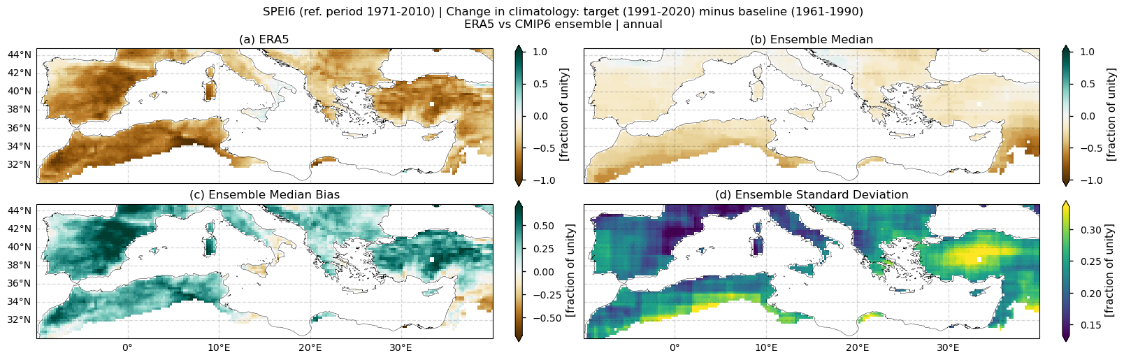
../../_images/51ad30ec921c8e83f987c838af2c62cc4bef72714b5eb26072c775f43f46b94e.png

Fig 1. Spatial patterns of SPEI6 change over the Mediterranean region. Panels show (a) ERA5 reference, (b) CMIP6 ensemble median (median of the selected subset of models at each grid cell), (c) ensemble median bias relative to ERA5, and (d) ensemble spread (standard deviation across the selected models). SPEI6 is standardised over the reference period 1971–2010. SPEI6 change is calculated at each grid point as the difference between the monthly climatologies of the target period (1991–2020) and the baseline period (1961–1990), and then averaged to obtain the annual mean.

3.3. Plot model maps#

In this section, we invoke the plot_models() function to visualise the SPEI6 change of every model individually. Note that the model data used in this section maintains its original grid.

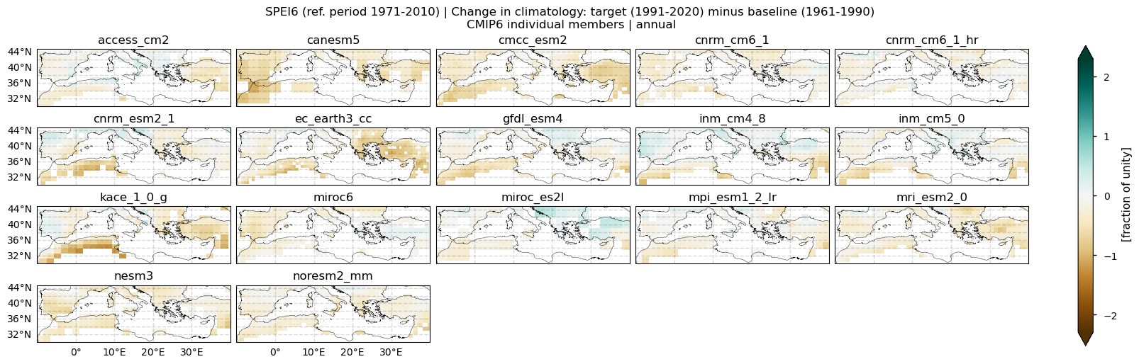
../../_images/707e13e8de5e293edf24ec1a2225b6cb634a658b639fa61647a2aaa9c8198ac1.png

Fig 2. Spatial patterns of SPEI6 change for each individual CMIP6 model over the Mediterranean region. SPEI6 is standardised over the reference period 1971–2010. For each model, SPEI6 change is calculated at each grid point as the difference between the monthly climatologies of the target period (1991–2020) and the baseline period (1961–1990), and then averaged to obtain the annual mean.

3.4. Plot bias maps#

In this section, we invoke the plot_models() function to visualise the bias of the vSPEI6 change for every model individually. Note that the model data used in this section has previously been interpolated to the ERA5 grid. Regridding is performed for each essential climate variable before the index calculation to preserve standardisation.

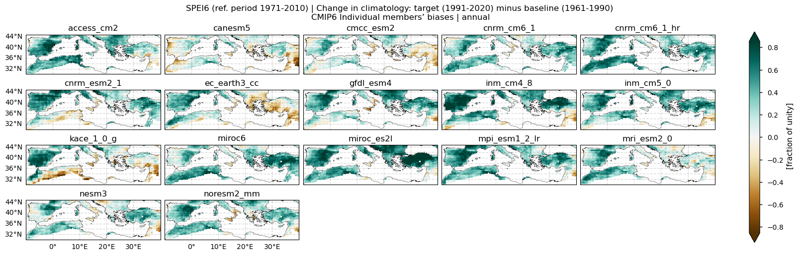
../../_images/b4a60afa83cd4a1eb36346c86520245fdd5c0641b9e1f6e8fb0107ff4e6590fc.png

Fig 3. Bias of SPEI6 change for each individual CMIP6 model relative to ERA5 over the Mediterranean region. SPEI6 is standardised over the reference period 1971–2010. For each model and ERA5, SPEI6 change is calculated at each grid point as the difference between the monthly climatologies of the target period (1991–2020) and the baseline period (1961–1990), and then averaged to obtain the annual mean.

3.5. Timeseries#

This section examines the time series of SPEI6 anomalies relative to the baseline climatology. We first use compute_change_4timeseries(), which calculates SPEI6 anomalies for each month of the timeseries (relative to the baseline climatology of each month) and aggregates them according to the time_agg parameter. Spatially averaged values are then obtained. Light grey shading highlights the baseline period, while darker grey shading marks the target period. The analysis compares the CMIP6 ensemble median, ERA5, and individual models, displaying trends for both ERA5 and the ensemble median. Additionally, it shows the ensemble spread and the slope values of the trends for ERA5 and the CMIP6 ensemble median.

Show code cell source

Hide code cell source

# Define colors
colors = {"CMIP6": "green", "ERA5": "black"}

# Cutout region
regionalise_kwargs = {
    "lon_slice": slice(area[1], area[3]),
    "lat_slice": slice(area[0], area[2]),
}

# Compute the change/anomaly for ERA5
ds_era5_change = compute_change_4timeseries(ds_era5, baseline_slice, time_agg)

# Regionalise and compute spatially weighted mean
era5_mean = diagnostics.spatial_weighted_mean(
    utils.regionalise(ds_era5_change, **regionalise_kwargs)
)
era5_mean["year"]=pd.to_datetime(era5_mean["year"].values, format='%Y')


# Compute change/anomaly for each model and spatially aggregate
cmip6_means = []
for model, ds in model_datasets.items():
    ds_model_change = compute_change_4timeseries(ds, baseline_slice, time_agg)
    ds_model_change["year"]=pd.to_datetime(ds_model_change["year"].values, format='%Y')
    ds_model_regional = utils.regionalise(ds_model_change, **regionalise_kwargs)
    cmip6_mean = diagnostics.spatial_weighted_mean(ds_model_regional)
    cmip6_means.append(cmip6_mean)

# Ensemble statistics
cmip6_stack = xr.concat(cmip6_means, dim="model")
cmip6_var = cmip6_stack.median("model", keep_attrs=True)
cmip6_std = cmip6_stack.std("model", keep_attrs=True)

# Initialize plot
plt.figure(figsize=(10, 5))

# Plot individual model time series
for model_data in cmip6_means:
    model_values = model_data.values.flatten() if model_data.ndim > 1 else model_data.values
    plt.plot(model_data['year'], model_values, linestyle='-', color="grey", alpha=0.4)

# Add legend entry for individual models
plt.plot([], [], linestyle='-', color='grey', alpha=0.3, label='Individual Models')

# Plot ERA5
era5_mean.plot(label="ERA5", color=colors["ERA5"])

# Plot CMIP6 median
cmip6_var.plot(label="CMIP6 Median", color=colors["CMIP6"])

# Fill ±1 std (spread)
plt.fill_between(
    cmip6_var['year'],
    cmip6_var.values - cmip6_std.values,
    cmip6_var.values + cmip6_std.values,
    color = colors["CMIP6"],
    alpha = 0.5,
    label = "CMIP6 Spread"
)

# Compute trends
slope_era5, p_value_era5 = plot_trend(
    era5_mean['year'][~np.isnan(era5_mean.values)],
    era5_mean.values[~np.isnan(era5_mean.values)],
    "ERA5 Trend",
    colors["ERA5"]
)

slope_cmip6, p_value_cmip6 = plot_trend(
    cmip6_var['year'][~np.isnan(cmip6_var.values)],
    cmip6_var.values[~np.isnan(cmip6_var.values)],
    "CMIP6 Median Trend",
    colors["CMIP6"]
)

trend_info = [
    ("ERA5", slope_era5, p_value_era5),
    ("CMIP6 Median", slope_cmip6, p_value_cmip6)
]

# Labels and grid
plt.xlabel('Year')
plt.ylabel("Fraction of unity")
title = (f"SPEI{window} (ref. period {reference_slice.start}-{reference_slice.stop}) | Change rel. to {baseline_slice.start}-{baseline_slice.stop}\n"
        f"Target period: ({target_slice.start}-{target_slice.stop}) | {time_agg}")

plt.title(title)

    
plt.legend()
plt.grid(True)

# Format x-axis as years
ax = plt.gca()
ax.xaxis.set_major_formatter(mdates.DateFormatter('%Y'))
plt.gcf().autofmt_xdate()

# Annotate trends
plt.gcf().text(
    0.5, -0.015,
    '\n'.join([
        f"{name} Trend: {trend:.4f} (fraction of unity/decade), p-value: {p:.3e}"
        for name, trend, p in trend_info
    ]),
    fontsize=12,
    ha='center',
    va='center',
    bbox=dict(boxstyle="square,pad=0.5", edgecolor="black", facecolor="lightgray")
)

plt.ylim((-1.7, 1.7))
# Shade baseline period (light gray)
ax.axvspan(
    pd.to_datetime(str(baseline_slice.start)),
    pd.to_datetime(str(baseline_slice.stop)),
    color="lightgray",
    alpha=0.5,
    label="Baseline period"
)

# Shade target period (grey)
ax.axvspan(
    pd.to_datetime(str(target_slice.start)),
    pd.to_datetime(str(target_slice.stop)),
    color="grey",
    alpha=0.3,
    label="Target period"
)
plt.show()

../../_images/f749e4e64faf42d112ee8fa50e091a31a85f8d2b0df1443dc5486715826a0e13.png

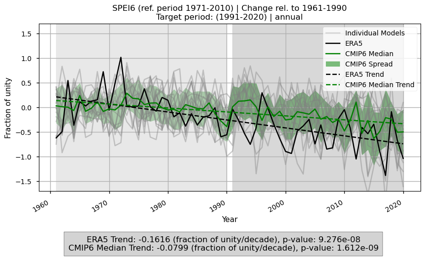
Fig 4. Time series of SPEI6 anomalies over the Mediterranean region, calculated relative to the baseline climatology. Monthly anomalies are aggregated according to the specified timescale and then spatially averaged over the region. Light grey shading indicates the baseline period, and dark grey shading indicates the target period. The figure compares ERA5, the CMIP6 ensemble median, and individual models, showing trends for ERA5 and the ensemble median, as well as the ensemble spread and slope values of the trends.

3.6. Results summary#

ERA5 indicates a general intensification of drought conditions over the Mediterranean region when comparing the baseline (1961–1990) and target (1991–2020) periods.
The CMIP6 ensemble median captures this SPEI6 change signal, but the magnitude of the increase in drought conditions is underestimated, particularly over eastern Spain, southern France, and much of Turkey.
With respect to inter-model spread, models do not reproduce the same spatial pattern. The largest spread appears over North African countries bordering the Mediterranean, Turkey, Lebanon, and Syria, and to a lesser extent over the Balkans, Portugal, and central and western Spain.
Time series of spatial means over the Mediterranean confirm this increase in drought conditions and the underestimation by CMIP6 models, with trends of –0.15 for ERA5 and –0.08 (about half) for the CMIP6 median.

3.7. Implications for the users#

Models do not reproduce the same exact spatial pattern, but the ensemble median captures the SPEI6 change. This underlines the importance of considering large ensembles rather than relying on a single or a few models.
Although the CMIP6 ensemble median captures the intensification of drought conditions, caution is needed when looking into the future. Precipitation projections generally involve more uncertainty than temperature, and model biases may evolve under changing climate conditions [9].
This assessment shows consistent results with those obtained in the C3S Atlas. In addition, it provides users with insight into the rationale behind SPEI and how models reproduce historical conditions over the Mediterranean, reinforcing its value as a tool for water management and drought preparedness.
The pronounced inter-model spread over North Africa, Turkey, and the eastern Mediterranean implies that users in these regions may face higher future uncertainty. This highlights the need to stress-test adaptation strategies against a wide range of plausible futures rather than relying on a single scenario.

ℹ️ If you want to know more#

Key resources#

Some key resources and further reading were linked throughout this assessment.

The CDS catalogue entries for the data used were:

CMIP6 climate projections (daily - daily maximum near-surface air temperature, daily minimum near-surface air temperature and precipitation): https://cds.climate.copernicus.eu/datasets/projections-cmip6?tab=overview
ERA5 hourly data on single levels from 1940 to present (2m temperature and total precipitation): https://cds.climate.copernicus.eu/datasets/reanalysis-era5-pressure-levels-monthly-means?tab=overview

Code libraries used:

C3S EQC custom functions, c3s_eqc_automatic_quality_control, prepared by B-Open

References#

[1] Vicente-Serrano, S. M., Beguerı́a, S., and López-Moreno, J. I., 2010. A multiscalar drought index sensitive to global warming: The standardized precipitation evapotranspiration index, Journal of Climate, 23, 1696–1718. https://doi.org/10.1175/2009JCLI2909.1

[2] Wilhite, D. A., 2000. Droughts as a natural hazard: concepts and definitions. In: DROUGHT, A Global Assessment, vol. I and II, Routledge Hazards and Disasters Series, Routledge.

[3] Vicente-Serrano, S. M., Beguerı́a, S., Lorenzo-Lacruz, J., Camarero, J. J., López-Moreno, J. I., Azorin-Molina, C., Revuelto, J., Morán-Tejeda, E., and Sanchez-Lorenzo, A., 2012. Performance of drought indices for ecological, agricultural, and hydrological applications, Earth Interactions, 16, https://doi.org/10.1175/2012EI000434.1

[4] Yao, N., Li, L., Feng, P., Feng, H., Liu, D. L., Liu, Y., Jiang, K., Hu, X., and Li, Y., 2020. Projections of drought characteristics in China based on a standardized precipitation and evapotranspiration index and multiple GCMs. Science of The Total Environment, 704, 135245. https://doi.org/10.1016/j.scitotenv.2019.135245

[5] Tuong, V. Q., Kiet, B. A., and Pham, T. T., 2025. Assessment of Future Drought Characteristics Using Various Temporal Scales and Multiple Drought Indices over Mekong Basin Under Climate Changes. Water, 17(10), 1507. https://doi.org/10.3390/w17101507

[6] Iturbide, M., Gutiérrez, J. M., Alves, L. M., Bedia, J., Cerezo-Mota, R., Cimadevilla, E., Cofiño, A. S., Di Luca, A., Faria, S. H., Gorodetskaya, I. V., Hauser, M., Herrera, S., Hennessy, K., Hewitt, H. T., Jones, R. G., Krakovska, S., Manzanas, R., Martínez-Castro, D., Narisma, G. T., Nurhati, I. S., Pinto, I., Seneviratne, S. I., van den Hurk, B., and Vera, C. S., 2020. An update of IPCC climate reference regions for subcontinental analysis of climate model data: definition and aggregated datasets, Earth Syst. Sci. Data, 12, 2959–2970, https://doi.org/10.5194/essd-12-2959-2020

[7] Hargreaves, G. H., and Samani, Z. A., 1985. Reference crop evapotranspiration from temperature, Applied engineering in agriculture, pp. 96–99. https://doi.org/10.13031/2013.26773

[8] Beguerı́a, S., Vicente-Serrano, S. M., Reig, F., and Latorre, B., 2014. Standardized precipitation evapotranspiration index (spei) revisited: Parameter fitting, evapotranspiration models, tools, datasets and drought monitoring, International Journal of Climatology, 34, 3001–3023. https://doi.org/10.1002/joc.3887

[9] Schmith, T., Thejll, P., Berg, P., Boberg, F., Christensen, O. B., Christiansen, B., Christensen, J. H., Madsen, M. S., and Steger, C., 2021. Identifying robust bias adjustment methods for European extreme precipitation in a multi-model pseudo-reality setting, Hydrol. Earth Syst. Sci., 25, 273–290, https://doi.org/10.5194/hess-25-273-2021

CMIP6 biases in SPEI6 drought simulations over the Mediterranean region

Contents

5.1.1. CMIP6 biases in SPEI6 drought simulations over the Mediterranean region#

🌍 Use case: Investigating drought biases to inform water management#

❓ Quality assessment question#

📢 Quality assessment statement#

📋 Methodology#

📈 Analysis and results#

1. Parameters, requests and functions definition#

1.1. Import packages#

1.2. Define Parameters#

1.3. Define models#

1.4. Define ERA5 request#

1.5. Define model requests#

1.6. Functions to cache#

2. Downloading and processing#

2.1. Download and transform ERA5#

2.2. Download and transform models#

2.3. Apply land-sea mask and change some attributes#

3. Plot and describe results#

3.1. Define plotting functions#

3.2. Plot ensemble maps#

3.3. Plot model maps#

3.4. Plot bias maps#

3.5. Timeseries#

3.6. Results summary#

3.7. Implications for the users#

ℹ️ If you want to know more#

Key resources#

References#