Please note that this repository is used for development and review, so quality assessments should be considered work in progress until they are merged into the main branch

1.6.1. Suitability of satellite sea ice thickness level 4 data for estimating sea ice volume

Production date: 2026-06-30

Produced by: Timothy Williams, Nansen Environment and Remote Sensing Center

🌍 Use case: Assessing the suitability of the level-4 merged CryoSat-2/SMOS satellite sea ice thickness product for estimating sea ice volume

❓ Quality assessment question

How well can sea ice volume be estimated from the Level-4 merged CryoSat-2/SMOS (Soil Moisture and Ocean Salinity) satellite sea ice thickness product?

📢 Quality assessment statement

These are the key outcomes of this assessment

• The Level-4 sea ice thickness (SIT) product is well-suited to calculate sea ice volume in the winter months (it is not available in the summer months from May to September due to unresolved bias originating from melting snow or open melt ponds). This is mainly due to the filling of gaps between altimeter tracks (including the polar hole of latitudes exceeding 88\(^\circ\)N) having been achieved by optimal interpolation from CryoSat-2 and SMOS (Soil Moisture and Ocean Salinity) measurements.

• Calculated volumes are similar to reanalysis volumes, and in fact many reanalyses actually assimilate the Level-4 SIT product. There is no significant trend apparent over the period when it is available (14 winters, beginning Octobers 2010-2023).

📋 Methodology

We consider the sea ice thickness (SIT) dataset, which has one Level-4 product, made by using optimal interpolation (OI) to merge CryoSat-2 altimeter data with SMOS passive microwave data (Ricker et al, 2017). It dates from October 2010 to present. This dataset also has two Level-3 products based only on altimeter products, which have a lot of missing data making the calculation of sea ice volume from them much more difficult.

Note that in this analysis we use version 1.0 of the L4 product, which is no longer the latest version (currently 1.1) so results may change if the latest data are used.

To calculate the sea ice volume we also need the SSMIS (Special Sensor Microwave Imager/Sounder) data from the sea ice concentration (SIC) dataset. This data was used as auxiliary data for the Level-4 thickness product so the two products are consistent with each other. These products are both available on the same 25-km equal area grid (the EASE2 (Equal-Area Scalable Earth) grid) so once they have been downloaded, the sea ice volume in one grid cell (in km\(^3\)) is \(V=Ahc\), where \(h=\)SIT/1000 is the thickness converted from meters to kilometers, \(c=\)SIC/100 is the sea ice area fraction, and \(A=\)625 km\(^2\) is the grid cell area. The total sea ice volume can then be found by adding the volumes contained in each grid cell.

A rough estimate of the uncertainty in the volume can be obtained in a similar way, by assuming the SIT and SIC uncertainties are independent, and that spatial errors are uncorrelated between grid cells. The variance in each grid cell is given by \((\Delta V)^2 = A(c\Delta h)^2 + A(h\Delta c)^2\), and the variance of the total volume is then obtained by summing over all grid cells. The standard deviation of the total volume is then the square root of the total variance.

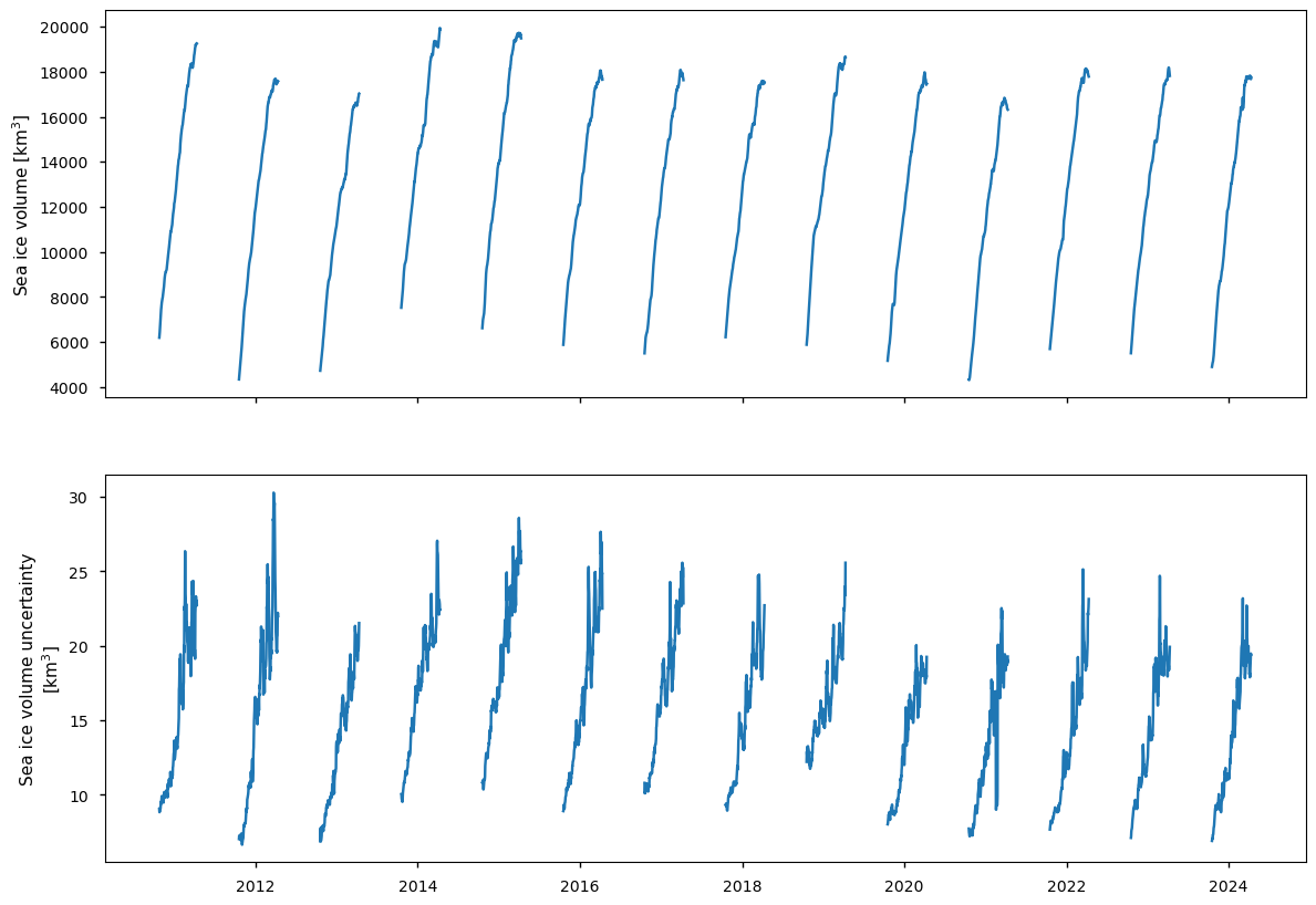
Time series of the volume and the uncertainties are plotted. The uncertainties estimated in the way described above are quite small in comparison to the total volume, and are likely underestimated, given the differences between it and independent thickness observations (Hendricks, 2023). The uncertainty estimation method is also inconsistent with the application of OI to make the Level-4 product, which used a correlation length scale (not provided with the product) to approximate the spatial correlation (Hendricks et al, 2023). A full uncertainty calculation could perhaps be computed with access to the individual Cryosat-2 freeboard data, and passive microwave SMOS and SIC data using a similar method to that used by Zygmontowska et al (2014), who used a Monte Carlo approach to estimate the uncertainty in sea ice volume from ICESat SIT data and SIC data. However, this would be extremely expensive computationally as the OI method would need to be run over many realisations of its input data (altimeter, SMOS, SIC, snow, ice density). Zygmontowska et al (2014) found that uncertainty in snow depth was the biggest contributor uncertainty to the volume uncertainty, although the conversion from freeboard to thickness is different for Cryosat-2 which scatters from the snow-ice interface (ICESat scatters from the snow-air interface).

The “Analysis and results” section is structured as follows:

1. Parameters, requests and functions definition

2. Downloading and transformation of the data

3. Results

📈 Analysis and results

1. Parameters, requests and functions definition

• Define parameters and formulate requests for downloading with the EQC toolbox.

• Define functions to be applied to process and reduce the size of the downloaded data.

• Define functions to post-process and visualize the data.

1.1 Import libraries

Define code to import the required libraries

Show code cell source

Hide code cell source

import cartopy.crs as ccrs
import matplotlib.pyplot as plt
import xarray as xr
from c3s_eqc_automatic_quality_control import download, plot
import pandas as pd
import numpy as np
import calendar


plt.style.use("seaborn-v0_8-notebook")

# suppress xarray warning
_ = xr.set_options(use_new_combine_kwarg_defaults=True)

1.2 Set parameters

• Set the time range for ENVISAT data with year_start_envisat and year_stop_envisat

• Set the time range for CRYOSAT data with year_start_cryosat and year_stop_cryosat

Show code cell source

Hide code cell source

# start and stop for CS2-SMOS (start of winter for this date)
year_start = 2010
year_stop = 2023

1.3 Define function to cache

• download_siconc_data downloads the required SIC data to match the time period covered by the SIT data.

• moving_average applies a moving average with a window of 7 days to get a mean SIC that matches the time period covered by the SIT data.

• get_siconc_data combines the above functions to download, average and format the SIC data into a form that can be used by the get_sivol function, which does the volume calculation.

Show code cell source

Hide code cell source

def download_siconc_data(time_bnds):
    """
    Downloads SIC to match the time period covered by the SIT data, determined by its "time_bnds" variable
    
    Parameters
    ----------    
    time_bnds : xarray.DataArray
    """
    start = pd.Timestamp(time_bnds[0,0].values)
    stop = pd.Timestamp(time_bnds[-1,1].values)
    lims = [(start, stop)]

    # The SIC dataset changes from CDR to ICDR in 2021,
    # so may need to split the requests
    sic_icdr_start_year = 2021
    if start.year < sic_icdr_start_year and stop.year >= sic_icdr_start_year:
        lims = [
            (start, pd.Timestamp(sic_icdr_start_year - 1, 12, 31)),
            (pd.Timestamp(sic_icdr_start_year, 1, 1), stop),
        ]
    
    collection_id = "satellite-sea-ice-concentration"
    conc_request = {
        "variable": "all",
        "sensor": "ssmis",
        "region": "northern_hemisphere",
        "temporal_aggregation": "daily",
    }

    requests = []
    for start_, stop_ in lims:
        if start_.year < sic_icdr_start_year:
            request = conc_request | {"cdr_type": "cdr", "version": "3_1"}
        else:
            request = conc_request | {"cdr_type": "icdr", "version": "3_0"}
        
        requests += download.update_request_date(request, start = start_, stop = stop_, stringify_dates=True)

    return download.download_and_transform(collection_id, requests).sel(time=slice(start, stop))


def moving_average(ds):
    """
    Gets 7-day moving average of sea_ice_concentration (mean) and total_standard_uncertainty (rms)
    
    Parameters
    ----------
    ds : xarray.Dataset
    """
    # 7-day moving average for sea_ice_concentration (mean)
    sic_ma = ds['ice_conc'].rolling(time=7, center=True).mean()
    
    # 7-day moving average for total_standard_uncertainty (root mean square)
    tsu_ma = np.sqrt(
        (ds['total_standard_uncertainty'] ** 2).rolling(time=7, center=True).mean()
    )
    
    # Remove NaN time steps (edges from rolling window)
    #valid_times = ~(sic_ma.isnull().all(['yc', 'xc']))
    valid_times = slice(3, -3)

    result = {'ice_conc': sic_ma.isel(time=valid_times),
              'total_standard_uncertainty': tsu_ma.isel(time=valid_times)}
    return xr.Dataset(result)


def get_siconc_data(time_bnds, ds_download=None):
    """
    Parameters
    ----------
    time_bnds : xarray.DataArray
    ds_download : xarray.Dataset
        downloaded SIC data
    """
    if ds_download is None:
        ds_download = download_siconc_data(time_bnds)
    ds = moving_average(ds_download)
    ds["time"].attrs["bounds"] = "time_bnds"
    ds["time_bnds"] = time_bnds
    return ds


def get_sivol(ds, ds_sic=None):
    """
    Calculate sea ice volume and its uncertainty.
    
    Parameters
    ----------
    ds : xarray.Dataset
        Dataset containing sea ice thickness and uncertainty fields
    ds_sic:
        Dataset containing sea ice concentration and uncertainty fields (7-day moving average)
        
    Returns
    -------
    xarray.Dataset
        Dataset with sivol (volume) and sivol_uncertainty variables
    """
    # Get ice concentration data
    if ds_sic is None:
        ds_sic = get_siconc_data(ds["time_bnds"])
    
    # Grid resolution in km
    dx = np.diff(ds["xc"].values[:2])[0]
    grid_area = dx ** 2  # km^2
    
    # Extract variables
    sit = ds["sea_ice_thickness"]  # thickness (m)
    sit_unc = ds["uncertainty"]  # thickness uncertainty (m)
    sic = 1e-2 * ds_sic["ice_conc"]  # ice concentration (fraction)
    sic_unc = 1e-2 * ds_sic["total_standard_uncertainty"]  # concentration uncertainty (fraction)
    
    # Calculate volume
    sivol = grid_area * (sic * sit).sum(dim=("xc", "yc")) / 1e3  # km^3
    
    # Uncertainty propagation for product: V = A * sum(C * T)
    # For each grid cell: dV = A * sqrt((C*dT)^2 + (T*dC)^2)
    # Total uncertainty: combine in quadrature across all cells
    
    # Per-cell variance contributions
    var_from_thickness = (sic * sit_unc) ** 2
    var_from_concentration = (sit * sic_unc) ** 2
    
    # Total variance per cell
    total_var_per_cell = var_from_thickness + var_from_concentration
    
    # Sum variances across spatial dimensions (variances add)
    total_variance = total_var_per_cell.sum(dim=("xc", "yc")) #m^2
    
    # Standard uncertainty
    sivol_uncertainty = grid_area * np.sqrt(total_variance) / 1e3 # km^3
    
    # Create output dataset
    result = xr.Dataset({
        "sivol": sivol,
        "sivol_uncertainty": sivol_uncertainty
    })
    
    result["sivol"].attrs["units"] = "km$^3$"
    result["sivol"].attrs["long_name"] = "Sea ice volume"
    result["sivol_uncertainty"].attrs["units"] = "km$^3$"
    result["sivol_uncertainty"].attrs["long_name"] = "Sea ice volume uncertainty"
    result["sivol_uncertainty"].attrs["description"] = (
        "Combined uncertainty from ice concentration and thickness, "
        "propagated assuming independent random errors"
    )
    return result

1.4 Download wrapper functions

• download_and_get_sivol downloads the data for one winter and computes the sea ice volume with get_sivol, which is then stored on disk.

• download_examples downloads example records to plot maps and give a qualitative comparison between the Level-3 and Level-4 products.

Show code cell source

Hide code cell source

def download_and_get_sivol(winter_start_year):
    collection_id = "satellite-sea-ice-thickness"
    request = {
        "processing_level": "level_4",
        "satellite_mission": ["combined_product"],
        "variable": ["sea_ice_thickness"],
        "temporal_resolution": ["daily"],
        "version": "1_0",     
    }
    start = pd.Timestamp(winter_start_year, 10, 18)
    stop = pd.Timestamp(winter_start_year + 1, 4, 12)
    requests = download.update_request_date(request, start = start, stop = stop, stringify_dates=True)
    ds = download.download_and_transform(collection_id, requests, transform_func=get_sivol)
    return ds.sel(time=slice(start, stop))


def download_examples(year=2020, month=1):

    # calendar info
    years = [str(year)]
    months = [f"{month:02d}"]
    _, ndays = calendar.monthrange(year, month)
    days = [f"{d:02d}" for d in range(1, ndays + 1)]
    
    # download 1 record of CryoSat-2
    collection_id = "satellite-sea-ice-thickness"
    ds = download.download_and_transform(collection_id, {
        "processing_level": "level_3",
        "satellite_mission": ["cryosat_2"],
        "variable": ["sea_ice_thickness"],
        "temporal_resolution": ["monthly"],
        "year": years,
        "month": months,
        "version": "3_0",
    })

    # extract projection variable
    proj_name = "Lambert_Azimuthal_Grid"
    proj_var = xr.DataArray(attrs=ds[proj_name].attrs)

    # set the variables to keep and save their attributes for reassigning later
    varnames = ("sea_ice_thickness", "uncertainty")
    to_drop = [vname for vname in ds.data_vars if vname not in varnames]
    attrs = {vname: ds[vname].attrs for vname in varnames}

    # take mean to remove time dimension and tag as CryoSat-2
    datasets = [ds.drop_vars(to_drop).mean(dim='time').expand_dims(source=["CryoSat-2"])]

    # download 1 month of CS2-SMOS and get the mean of SIT and the RMS uncertainty (averaging over all the days in the month)
    ds = download.download_and_transform(collection_id, {
        "processing_level": "level_4",
        "satellite_mission": ["combined_product"],
        "variable": ["sea_ice_thickness"],
        "temporal_resolution": ["daily"],
        "year": years,
        "month": months,
        "day": days,
        "version": "1_0"
    }).drop_vars(to_drop)
    data = {
        "sea_ice_thickness": ds["sea_ice_thickness"].mean(dim='time'),
        "uncertainty": np.sqrt((ds["uncertainty"] ** 2).mean(dim='time')),
    }

    # tag as CS2-SMOS
    datasets += [xr.Dataset(data).expand_dims(source=["CS2-SMOS"])]

    # merge datasets
    ds = xr.concat(datasets, 'source')
    del datasets

    # set variable attributes
    for vname, vattrs in attrs.items():
        for attr_name in ("standard_name", "long_name", "units", "grid_mapping"):
            ds[vname].attrs[attr_name] = vattrs[attr_name]
    
    # return after adding the projection variable
    return ds.assign_coords({proj_name: proj_var})

1.5 Plotting functions

• get_dummy_dataset adds a dummy date in summer where the volume and its uncertainty are not numbers (numpy.nan) so that the plots of consecutive winters are split.

• plot_time_series plots times series of the sea ice volume and its uncertainty.

Show code cell source

Hide code cell source

def get_dummy_dataset(ds):
    year = ds.time.dt.year[-1].item()
    data = {var: ('time', [np.nan]) for var in ds.data_vars}
    return xr.Dataset(data).assign_coords({'time': [pd.Timestamp(year, 6, 1)]})


def plot_time_series(ds):
    fig, axs = plt.subplots(2,1, sharex=True, figsize=(14,10))
    ds['sivol'].plot(ax=axs[0])
    ds['sivol_uncertainty'].plot(ax=axs[1])
    for ax in axs:
        ax.set_xlabel('')
        ax.set_title('')


def plot_maps(ds_eg, vname, vmax):
    # projection
    proj = ccrs.Stereographic(central_latitude=90)
    # zoom in on variable to plot
    da = ds_eg[vname].isel(xc=slice(90,310), yc=slice(90,310))
    # plot CS2 and CS2-SMOS side-by-side
    facet_grid = plot.projected_map(da, cbar_kwargs={"pad" : .025, 'shrink': .45, 'extend': 'both'}, projection=proj,
            robust=True, col="source", vmax=vmax, show_stats=False, figsize=(12,8))
    facet_grid.set_titles(template="{value}, January 2020")

2. Downloading and transformation of the data

This is where the data is downloaded, transformed into a sea ice volume time series using get_sivol and saved to disk by the EQC toolbox. If the code is rerun the transformed data is loaded from the disk.

Show code cell source

Hide code cell source

datasets = []
for winter_start_year in range(year_start, year_stop + 1):
    print(f"Winter starting in October {winter_start_year}")
    try:
        ds = download_and_get_sivol(winter_start_year)
    except:
        print(f"Could not get sivol for {winter_start_year}")
        continue
    dummy = [] if len(datasets) == 0 else [get_dummy_dataset(ds)]
    datasets += dummy + [ds]
ds_vol = xr.concat(datasets, 'time')
del datasets

Show code cell source

Hide code cell source

ds_eg = download_examples()

3. Results

Below we do a short visual comparison of the Level-3 and Level-4 products (monthly aggregations and their uncertainties). We then plot time series of the sea ice volume and an estimate of its uncertainty, as derived from the Level-4 product.

3.1 Qualitative comparison of Level-3 and Level-4 products

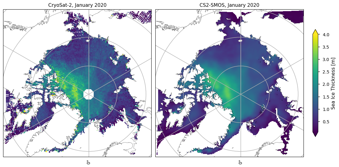
Below we show the SIT for the Level-3 product using only CryoSat-2 data (this is a mean of all the altimeter tracks crossing a grid cell in a month) and the Level-4 product which merges CryoSat-2 and SMOS data (the Level-4 data, which is provided daily, is averaged over one month). The SIT are similar in the areas with thicker ice (when the altimeter is more reliable), but gaps have been filled in the Level-4 product by the optimal interpolation (OI). The OI has also made the SIT much smoother.

Show code cell source

Hide code cell source

plot_maps(ds_eg, "sea_ice_thickness", vmax=4)

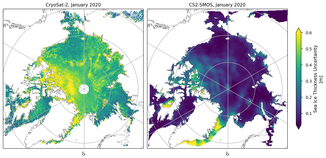
Below we show the uncertainty in SIT for the Level-3 product and the RMS uncertainty in the Level-4 product which merges CryoSat-2 and SMOS data. (Since the Level-4 product is provided daily, we take the RMS value over the whole month.) The OI, which partly aims to minimise uncertainty, has approximately halved the uncertainty of the Level-4 product compared to the Level-3 product.

Show code cell source

Hide code cell source

plot_maps(ds_eg, "uncertainty", vmax=.6)

3.2 Time series of sea ice volume and its uncertainty

Below we plot the time series of the sea ice volume and its uncertainty (the standard deviation of the total volume) as derived from the Level-4 product.

The commonly-used reference reanalysis PIOMAS (Pan-Arctic Ice Ocean Modeling and Assimilation System) and a machine-learning product (Edel et al, 2024)) have similar volumes in 2010-2020 to the ones shown below. (Note that PIOMAS assimilates CS2-SMOS data, while the model of Edel et al (2024) use the innovations from assimilating it to correct biases in years before it became available. The paper of Edel et al (2024) shows volumes for a longer time-series (1991-2020) and shows a drop in volume over that period, while there does not seem to be a significant trend in the volume over the period where CS2-SMOS data is available (14 winters beginning in Octobers 2010-2023), and quite large interannual variability.

This raises the question of whether 14 years is too short to capture a significant trend. However, Ludwig et al (2025, under review) compared several different thickness datasets (including CS2-SMOS). They also found that there was no trend in mean thickness (a similar quantity to volume) from 2010-2023, and tested the robustness of this claim against longer time series - including the two mentioned above (PIOMAS, Edel et al, 2024) - by calculating trends for different 13-year intervals and testing their statistical significance. They found significant (downward) trends for some of these intervals, concluding that 13 years is not too short a period to detect a significant trend if one is present.

Show code cell source

Hide code cell source

plot_time_series(ds_vol)

ℹ️ If you want to know more

Key resources

Introductory sea ice materials:

• Role of sea ice in the climate

• Sea ice as an indicator of climate change

• Observing sea ice with satellites

Code libraries used:

• C3S EQC custom functions, c3s_eqc_automatic_quality_control, prepared by B-Open.

References

[1] Ricker, R., Hendricks, S., Kaleschke, L., Tian-Kunze, X., King, J., & Haas, C. (2017). A weekly Arctic sea-ice thickness data record from merged CryoSat-2 and SMOS satellite data. The Cryosphere, 11(4), 1607-1623, https://doi.org/10.5194/tc-11-1607-2017

[2] Hendricks, S., Ricker, R., Kaleschke, L., Tian-Kunze, X. (2023) Sea Ice Thickness - CryoSat-2/SMOS Version 1.0: Algorithm Theoretical Basis Document. Copernicus Climate Change Service, Document reference: WP2-FDDP-2022-09_C3S2-Lot3_ATBD-of-v1.0-SeaIceThickness-CS2SMOS-product_v1.1, https://dast.copernicus-climate.eu/documents/satellite-sea-ice-thickness/level-4/v1-0/WP2-FDDP-2022-09_C3S2-Lot3_ATBD-of-v1.0-SeaIceThickness-CS2SMOS-product_1.1_final.pdf

[3] Hendricks, S. (2023). Sea Ice Thickness – CryoSat2-2/SMOS, Version 1.0: Product Quality Assessment Report. Copernicus Climate Change Service, Document reference: WP2-FDDP-2022-09_C3S2-Lot3_PQAR-of-v1.0-SeaIceThickness-CS2SMOS-products_v1.1, https://dast.copernicus-climate.eu/documents/satellite-sea-ice-thickness/level-4/v1-0/WP2-FDDP-2022-09_C3S2-Lot3_PQAR-of-v1.0-SeaIceThickness-CS2SMOS-product_v1.1_final.pdf

[4] Ludwig, V., Ribere, C., Fleury, S., Haas, C., Tsamados, M. et al. (2026). Biases, Uncertainties, and Trends in Arctic Sea-Ice Thickness: A Cross-Product Analysis from 1995 to 2023. EGUsphere, 2026, 1-37, https://doi.org/10.5194/egusphere-2025-6201 .

[5] Zygmuntowska, M., Rampal, P., Ivanova, N., & Smedsrud, L. H. (2014). Uncertainties in Arctic sea ice thickness and volume: new estimates and implications for trends. The Cryosphere, 8(2), 705-720, https://doi.org/10.5194/tc-8-705-2014

[6] Edel, L., Xie, J., Korosov, A., Brajard, J., & Bertino, L. (2025). Reconstruction of Arctic sea ice thickness (1992–2010) based on a hybrid machine learning and data assimilation approach. The Cryosphere, 19(2), 731-752, https://doi.org/10.5194/tc-19-731-2025

[7] Soriot, C., Vancoppenolle, M., Prigent, C., Jimenez, C., & Frappart, F. (2024). Winter arctic sea ice volume decline: uncertainties reduced using passive microwave-based sea ice thickness. Scientific Reports, 14(1), 21000, https://doi.org/10.1038/s41598-024-70136-9