Assessment of the resolution of surface albedo satellite data for monitoring the Sahara desert

1.2.1. Assessment of the resolution of surface albedo satellite data for monitoring the Sahara desert#

Production date: 30-09-2024

Produced by: Consiglio Nazionale delle Ricerche (CNR )

🌍 Use case: Estimating desertification using surface albedo data#

❓ Quality assessment question#

• Can satellite albedo datasets be used to estimate the expansion of the Sahara desert?

The Sahara, Earth’s largest hot desert, has expanded in recent decades. Existing studies indicates a sustained enlargement of the dry zone on both annual and seasonal timescales [1]. This implies risks to ecosystems, pastoral livelihoods, food and water security, and infrastructure across North and West Africa. Multiple regional studies document intensified desertification pressures in precisely the areas our analysis targets: sand‐dune encroachment around Nouakchott in Mauritania [2]; degradation and desertification sensitivity along the Algerian steppe, Sahara margin, where large‐scale countermeasures such as the “Green Dam” have been evaluated [3]; dune reactivation and wind‐erosion impacts in Niger [4]; active dune migration in the Libyan Ubārī Sand Sea [5]; and increased mobile dunes around Lake Chad and northern Chad since the 1970s [6]. In this assessment, we test whether satellite‐derived surface albedo from the Copernicus CDS (10-daily, 1-km; SPOT-VGT/PROBA-V, v2) can monitor desert expansion signals by mapping spatial albedo patterns and their changes comparing the data for two year, the winter season 2006-2007 and 2019-2020 (November to February, NDJF). Evaluating desertification during the NDJF[FM1.1] (November-January-February) period is crucial because this is often the dry season in many regions, making it the most vulnerable time for desertification to worsen. Albedo is a suitable proxy for surface state in arid lands because brightening often accompanies exposure or stabilization of bare sands and crusts, while darkening may reflect seasonal greening or increased surface moisture. Using seasonally consistent composites and quality screening, we quantify “desert-like” area via albedo masks and compute area changes on the native grid. The results reveal a small net increase in very bright desert‐like area across the Sahara, with the largest gains concentrated in the western–central Sahara (notably Mali and Mauritania), [FM2.1]aligning with the independent evidence cited above [1–6]. This supports the use of CDS surface albedo data as a powerful tool for monitoring desertification dynamics and regional hotspots of change.

📢 Quality assessment statement#

These are the key outcomes of this assessment

The seasonal albedo maps provide a clear, side-by-side view of surface reflectance in two benchmark years, making spatial changes in bright, desert-like areas easy to spot.

📋 Methodology#

The methodology adopted for the analysis is split into the following steps:

1. Choose the data to use and set up the code

Import all the relevant packages.

2. Data loading and preparation

Load monthly albedo data
Dataset inspection and Sahara albedo extraction
QFLAG filtering + Plot helpers 3. Plot and describe the results.
Sahara study area maps with country names
Detecting and Visualizing Sahara Desert Expansion from Albedo (NDJF, 2006→2019)
Quantifying Desertification by Country within the Sahara Study Domain
Validate “new-desert” pixels and inspect their values
Pixel count analysis of albedo map plots – Summer 2006 vs 2019
Plot albedo change map (2019 − 2006)

Take-home messages

📈 Analysis and results#

1. Choose the data to use and set up the code#

Import all the relevant packages#

In this section, we import all the relevant packages required to run the notebook.

2. Data loading and preparation#

Load monthly albedo data#

satellite='spot'

100%|██████████| 8/8 [00:00<00:00,  9.86it/s]
/data/common/miniforge3/envs/wp5/lib/python3.12/site-packages/earthkit/data/readers/netcdf/fieldlist.py:202: FutureWarning: In a future version of xarray the default value for data_vars will change from data_vars='all' to data_vars=None. This is likely to lead to different results when multiple datasets have matching variables with overlapping values. To opt in to new defaults and get rid of these warnings now use `set_options(use_new_combine_kwarg_defaults=True) or set data_vars explicitly.
  return xr.open_mfdataset(

satellite='proba'

100%|██████████| 7/7 [00:00<00:00, 41.57it/s]
/data/common/miniforge3/envs/wp5/lib/python3.12/site-packages/earthkit/data/readers/netcdf/fieldlist.py:202: FutureWarning: In a future version of xarray the default value for data_vars will change from data_vars='all' to data_vars=None. This is likely to lead to different results when multiple datasets have matching variables with overlapping values. To opt in to new defaults and get rid of these warnings now use `set_options(use_new_combine_kwarg_defaults=True) or set data_vars explicitly.
  return xr.open_mfdataset(

Dataset inspection and Sahara albedo extraction#

=== SPOT ===
<xarray.Dataset> Size: 20GB
Dimensions:       (time: 96, latitude: 1456, longitude: 3920)
Coordinates:
  * time          (time) datetime64[ns] 768B 2006-01-10 ... 2013-12-10
  * latitude      (latitude) float64 12kB 28.0 27.99 27.98 ... 15.03 15.02 15.01
  * longitude     (longitude) float64 31kB -10.0 -9.991 -9.982 ... 24.98 24.99
Data variables:
    crs           (time) |S1 96B b'' b'' b'' b'' b'' b'' ... b'' b'' b'' b'' b''
    AL_BH_BB      (time, latitude, longitude) float32 2GB dask.array<chunksize=(1, 1456, 3920), meta=np.ndarray>
    AL_BH_BB_ERR  (time, latitude, longitude) float32 2GB dask.array<chunksize=(1, 1456, 3920), meta=np.ndarray>
    AL_BH_NI      (time, latitude, longitude) float32 2GB dask.array<chunksize=(1, 1456, 3920), meta=np.ndarray>
    AL_BH_NI_ERR  (time, latitude, longitude) float32 2GB dask.array<chunksize=(1, 1456, 3920), meta=np.ndarray>
    AL_BH_VI      (time, latitude, longitude) float32 2GB dask.array<chunksize=(1, 1456, 3920), meta=np.ndarray>
    AL_BH_VI_ERR  (time, latitude, longitude) float32 2GB dask.array<chunksize=(1, 1456, 3920), meta=np.ndarray>
    AGE           (time, latitude, longitude) float32 2GB dask.array<chunksize=(1, 1456, 3920), meta=np.ndarray>
    NMOD          (time, latitude, longitude) float32 2GB dask.array<chunksize=(1, 1456, 3920), meta=np.ndarray>
    QFLAG         (time, latitude, longitude) float32 2GB dask.array<chunksize=(1, 1456, 3920), meta=np.ndarray>
Attributes: (12/23)
    time_coverage_end:    2006-01-10T23:59:59Z
    time_coverage_start:  2005-12-21T00:00:00Z
    platform:             SPOT-5
    sensor:               VEGETATION-2
    Conventions:          CF-1.6
    archive_facility:     VITO
    ...                   ...
    source:               Derived from EO satellite imagery
    title:                10 daily broadband hemispherical surface albedo der...
    creator_name:         Iskander Benhadj
    creator_email:        iskander.benhadj@vito.be
    project:              C3S_312b_Lot5
    date_created:         2021-03-24

=== PROBA ===
<xarray.Dataset> Size: 16GB
Dimensions:       (time: 78, latitude: 1456, longitude: 3920)
Coordinates:
  * time          (time) datetime64[ns] 624B 2014-01-10 ... 2020-06-10
  * latitude      (latitude) float64 12kB 28.0 27.99 27.98 ... 15.03 15.02 15.01
  * longitude     (longitude) float64 31kB -10.0 -9.991 -9.982 ... 24.98 24.99
Data variables:
    crs           (time) |S1 78B b'' b'' b'' b'' b'' b'' ... b'' b'' b'' b'' b''
    AL_BH_BB      (time, latitude, longitude) float32 2GB dask.array<chunksize=(1, 1456, 3920), meta=np.ndarray>
    AL_BH_BB_ERR  (time, latitude, longitude) float32 2GB dask.array<chunksize=(1, 1456, 3920), meta=np.ndarray>
    AL_BH_NI      (time, latitude, longitude) float32 2GB dask.array<chunksize=(1, 1456, 3920), meta=np.ndarray>
    AL_BH_NI_ERR  (time, latitude, longitude) float32 2GB dask.array<chunksize=(1, 1456, 3920), meta=np.ndarray>
    AL_BH_VI      (time, latitude, longitude) float32 2GB dask.array<chunksize=(1, 1456, 3920), meta=np.ndarray>
    AL_BH_VI_ERR  (time, latitude, longitude) float32 2GB dask.array<chunksize=(1, 1456, 3920), meta=np.ndarray>
    AGE           (time, latitude, longitude) float32 2GB dask.array<chunksize=(1, 1456, 3920), meta=np.ndarray>
    NMOD          (time, latitude, longitude) float32 2GB dask.array<chunksize=(1, 1456, 3920), meta=np.ndarray>
    QFLAG         (time, latitude, longitude) float32 2GB dask.array<chunksize=(1, 1456, 3920), meta=np.ndarray>
Attributes: (12/23)
    time_coverage_end:    2014-01-10T23:59:59Z
    time_coverage_start:  2013-12-21T00:00:00Z
    platform:             PROBA-V
    sensor:               VEGETATION
    Conventions:          CF-1.6
    archive_facility:     VITO
    ...                   ...
    source:               Derived from EO satellite imagery
    title:                10 daily broadband hemispherical surface albedo der...
    creator_name:         Iskander Benhadj
    creator_email:        iskander.benhadj@vito.be
    project:              C3S_312b_Lot5
    date_created:         2021-03-31

QFLAG filtering + Plot helpers#

Show code cell source

Hide code cell source

def qc_bits47(da_albedo: xr.DataArray, qflag: xr.DataArray) -> xr.DataArray:
    """
    Keep pixels where:
      Bit 4 == 0  (no missing/invalid input)
      Bit 7 == 0  (albedo processing OK)
    """
    q = qflag.astype("int")
    bit4_ok = (q & 16)  == 0     # 2**4
    bit7_ok = (q & 128) == 0     # 2**7
    return da_albedo.where(bit4_ok & bit7_ok)

def seasonal_mean_bits47(ds: xr.Dataset, months, year, also_require_bb_ok=False) -> xr.DataArray:
    """QC (bits 4 & 7 [+ optional bit 9]) → select months in `year` → mean over time."""
    da = ds["AL_BH_BB"]
    q  = ds["QFLAG"].astype("int")
    # base QC
    ok = ((q & 16) == 0) & ((q & 128) == 0)        # bits 4 and 7 clear
    if also_require_bb_ok:
        ok = ok & ((q & 256) == 0)                 # bit 9 clear
    da = da.where(ok)
    sel = da.sel(time=da.time.dt.year == year).where(da.time.dt.month.isin(months), drop=True)
    return sel.mean("time", skipna=True)

def compute_extent(da: xr.DataArray, pad=0.3):
    lon0, lon1 = float(da.longitude.min()), float(da.longitude.max())
    lat0, lat1 = float(da.latitude.min()),  float(da.latitude.max())
    return [lon0 - pad, lon1 + pad, lat0 - pad, lat1 + pad]
def panel_map(ax, da, title, extent, proj, vmin, vmax, thr=None, valid_mask=None):
    im = da.plot.pcolormesh(ax=ax, transform=proj, cmap="cividis",
                            vmin=vmin, vmax=vmax, add_colorbar=False)
    ax.set_title(title)
    ax.set_extent(extent, crs=proj)
    ax.coastlines(resolution="10m", linewidth=0.7)
    ax.add_feature(cfeature.BORDERS, linewidth=0.4)
    if thr is not None:
        cs = da.plot.contour(ax=ax, transform=proj, levels=[thr],
                             colors="white", linewidths=1.1, add_colorbar=False)
        ax.clabel(cs, fmt=f"{thr:.2f}", inline=True, fontsize=8)
    # labels on left & bottom only (since colorbar is on the right)
    gl = ax.gridlines(draw_labels=True, linestyle=":", alpha=0.5,
                      x_inline=False, y_inline=False)
    gl.top_labels = False
    gl.right_labels = False
    gl.left_labels  = True
    gl.bottom_labels = True
    return im

def gridcell_areas_km2(lat, lon):
    R = 6371.0088
    latr = np.deg2rad(lat.values); lonr = np.deg2rad(lon.values)
    lat_e = np.concatenate(([latr[0] - (latr[1]-latr[0])/2],
                            (latr[:-1]+latr[1:])/2,
                            [latr[-1] + (latr[-1]-latr[-2])/2]))
    lon_e = np.concatenate(([lonr[0] - (lonr[1]-lonr[0])/2],
                            (lonr[:-1]+lonr[1:])/2,
                                [lonr[-1] + (lonr[-1]-lonr[-2])/2]))
    lat1, lat2 = lat_e[:-1][:,None], lat_e[1:][:,None]
    lon1, lon2 = lon_e[:-1][None,:], lon_e[1:][None,:]
    return R**2 * np.abs(np.sin(lat2)-np.sin(lat1)) * np.abs(lon2-lon1)

3. Plot and describe the results.#

Sahara study area maps with country names#

Show code cell source

Hide code cell source

BBOX = [28.0, -10.0, 15.0, 25.0]
n, w, s, e = BBOX
proj = ccrs.PlateCarree()
study_poly = box(w, s, e, n)
study_gdf = gpd.GeoDataFrame(geometry=[study_poly], crs="EPSG:4326")

shp = shapereader.natural_earth(resolution="50m", category="cultural", name="admin_0_countries")
countries = gpd.read_file(shp).to_crs("EPSG:4326")
name_col = "NAME_EN" if "NAME_EN" in countries.columns else "NAME"

target_names = {
    "Mali", "Mauritania", "Algeria", "Niger", "Libya", "Chad",
    "Western Sahara", "Morocco", "Burkina Faso", "Sudan", "Egypt"
}

countries = countries[countries[name_col].isin(target_names) & countries.intersects(study_poly)].copy()
countries["geom_clip"] = countries.geometry.intersection(study_poly)
countries = countries.set_geometry("geom_clip").reset_index(drop=True)


countries["rep_pt"] = countries.geometry.representative_point()
countries["NAME_USE"] = countries[name_col]
manual_pos = {
   
    "Western Sahara": (-9.6, 24.9),  
    "Morocco":        (-9.8, 27.3),  
    "Egypt":          (24.4, 26.0),  
    "Sudan":          (24.3, 16.6),  
}

nudges = {
    "Burkina Faso": (0.0, -0.3),
    "Mauritania":   (-0.3,  0.2),
}

outside_labels = set()  

fig, (ax1, ax2) = plt.subplots(
    1, 2, figsize=(12, 6),
    subplot_kw={"projection": proj},
    constrained_layout=True
)

ax1.set_extent([-20, 35, 5, 35], crs=proj)  # [W, E, S, N]
ax1.add_feature(cfeature.LAND, color="lightgray")
ax1.add_feature(cfeature.OCEAN, color="lightblue")
ax1.add_feature(cfeature.COASTLINE, linewidth=0.8)
ax1.add_feature(cfeature.BORDERS, linewidth=0.4)
study_gdf.boundary.plot(ax=ax1, color="red", linewidth=2)
ax1.set_title("Sahara Context with Study Area")
gl1 = ax1.gridlines(draw_labels=True, linestyle="--", color="gray", alpha=0.5)
gl1.top_labels = False; gl1.right_labels = False

# --- Right: zoomed study area with country names
ax2.set_extent([w, e, s, n], crs=proj)
ax2.add_feature(cfeature.LAND, color="lightgray")
ax2.add_feature(cfeature.OCEAN, color="lightblue")
ax2.add_feature(cfeature.COASTLINE, linewidth=0.8)
ax2.add_feature(cfeature.BORDERS, linewidth=0.5)


study_gdf.boundary.plot(ax=ax2, color="firebrick", linewidth=2)
countries.boundary.plot(ax=ax2, color="dimgray", linewidth=0.6)


for _, row in countries.iterrows():
    name = row["NAME_USE"]
    x0, y0 = row["rep_pt"].x, row["rep_pt"].y

   
    if name in manual_pos:
        x_lab, y_lab = manual_pos[name]
    else:
        dx, dy = nudges.get(name, (0.0, 0.0))
        x_lab, y_lab = x0 + dx, y0 + dy

    if name in outside_labels:
        x_out = e + 0.6  # outside right margin
        ax2.plot([x0, x_out - 0.15], [y0, y_lab], transform=proj, color="k", linewidth=0.6, alpha=0.8)
        x_lab = x_out

    ax2.text(
        x_lab, y_lab, name,
        transform=proj, ha="center", va="center",
        fontsize=9, weight="bold", color="black",
        bbox=dict(boxstyle="round,pad=0.2", fc="white", ec="none", alpha=0.75),
        zorder=5,
    )

ax2.set_title("Study Area with Country Names")
gl2 = ax2.gridlines(draw_labels=True, linestyle="--", color="gray", alpha=0.5)
gl2.top_labels = False; gl2.right_labels = False

plt.show()

../../_images/993be6b54652f096c3a21e5a8b9f30932eecc02cd6ede8a7810ed0b459838c81.png

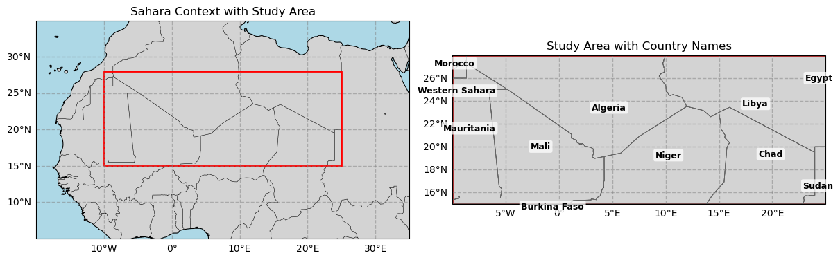
Figure 1. Study domain for the Sahara analysis. Left: West Africa context with the red rectangle showing the bounding box used for data extraction (28°N–15°N, 10°W–25°E; Plate Carrée). Right: Zoomed view of the box with national borders and labels (Morocco, Western Sahara, Mauritania, Mali, Algeria, Niger, Libya, Chad, Sudan, Egypt, and Burkina Faso) to indicate where changes are assessed.

Detecting and Visualizing Sahara Desert Expansion from Albedo (NDJF, 2006→2019)#

We build NDJF (Nov–Feb) albedo composites for two epochs—2006 from SPOT and 2019 from PROBA—using the same QC mask (Bits 4 & 7) via seasonal_mean_bits47. If 2019 NDJF is incomplete, we fall back to the latest available PROBA year. We then restrict all comparisons to the common valid footprint (valid_both). Pixel-wise change is computed as Δ = PROBA − SPOT. A pixel is flagged as “new desert” when (i) it was not desert in 2006, (ii) it is desert in 2019, and (iii) it brightened by at least min_delta = 0.02. “Desert” here means broadband hemispherical albedo > thr = 0.35. For context, we also mark pixels that brightened by >0.02 but remained below the threshold. Finally, the figure shows: (top left/right) the two NDJF albedo maps on a shared color scale with the threshold contour; and (bottom) a change map where red pixels are “new desert” (crossed the threshold), and pale yellow pixels brightened but stayed sub-threshold. Grid labels are placed on the left of the SPOT map and the right of the PROBA map for readability, and a single colorbar applies to both top panels.

Show code cell source

Hide code cell source

fig = plt.figure(figsize=(12, 10))
gs  = GridSpec(
    3, 2,
    width_ratios=[30, 1],      # narrow right column for colorbar
    height_ratios=[1, 1, 1.25],
    hspace=0.28, wspace=0.25
)

fig.suptitle(
    f"Sahara — NDJF Albedo (QC: Bits 4 & 7) — Left: {year_spot} (SPOT) | Right: {year_proba} (PROBA)",
    y=0.98, fontsize=14
)


ax1 = fig.add_subplot(gs[0, 0], projection=proj)
_   = panel_map(ax1, spot_map, f"{year_spot} (SPOT)", extent, proj, vmin, vmax, thr=thr, valid_mask=valid_both)


ax2 = fig.add_subplot(gs[1, 0], projection=proj)
im2 = panel_map(ax2, proba_map, f"{year_proba} (PROBA)", extent, proj, vmin, vmax, thr=thr, valid_mask=valid_both)

cax = fig.add_subplot(gs[0:2, 1])
cbar = fig.colorbar(im2, cax=cax)
cbar.set_label("Albedo")

from scipy.ndimage import binary_dilation


YELLOW_GROW_ITERS = 2
yellow_big = binary_dilation(brightened_below_thr, iterations=YELLOW_GROW_ITERS)


ax3 = fig.add_subplot(gs[2, :], projection=proj)
ax3.set_extent(extent, crs=proj)
ax3.coastlines("10m", linewidth=0.7); ax3.add_feature(cfeature.BORDERS, linewidth=0.4)
ax3.set_title(f"New desert (NDJF): crossed {thr:.2f} and brightened by > {min_delta:.02f}   —   {year_spot} → {year_proba}")


ax3.pcolormesh(spot_map.longitude, spot_map.latitude,
               np.where(valid_both, 0, np.nan), transform=proj,
               cmap="Greys", vmin=0, vmax=1, alpha=0.05)


ax3.scatter(nd_lon, nd_lat, s=24, c="#d73027", marker="s", lw=0, alpha=0.95,
            transform=proj, zorder=3, rasterized=True, label="New desert: crossed > threshold")
ax3.scatter(br_lon, br_lat, s=24, c="#ffd27f", marker="s", lw=0, alpha=0.9,
            transform=proj, zorder=2, rasterized=True, label="Brightened (< threshold)")

gl3 = ax3.gridlines(draw_labels=True, linestyle=":", alpha=0.5, x_inline=False, y_inline=False)
gl3.top_labels=False; gl3.left_labels=True; gl3.right_labels=True; gl3.bottom_labels=True

ax3.legend(loc="lower left", frameon=True, framealpha=0.95)
plt.show()

../../_images/2c454ffe47c92ab6523b80920633a9188e14321122594a875ec24ceae0991037.png

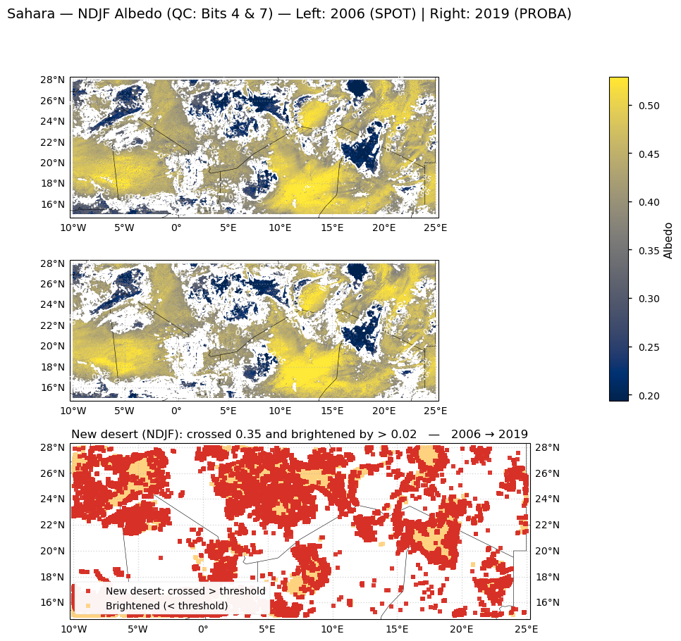
Figure 2. NDJF (Nov–Feb) broadband albedo over the Sahara in 2006 (SPOT, left) and 2019 (PROBA-V, right) after quality control (QFLAG bits 4 & 7: valid inputs and algorithm success). The lower panel highlights change between the two epochs: red pixels brightened by >0.02 and crossed above the 0.35 threshold (“new desert”), while yellow pixels brightened by >0.02 but remained below the threshold. Only the footprint valid in both years is considered.

Quantifying desertification by country within the Sahara study domain#

To quantify desertification in each country inside the Sahara study domain, we (i) mapped pixels that became newly “desert-like” between 2006 and 2019 (crossing an albedo threshold in 2019 but not in 2006) after quality control, (ii) summed those pixels to km² using an equal-area projection, and (iii) normalized by each country’s own area within the study box to report an interpretable percentage of its in-box territory affected. To avoid distorted ratios from tiny border slivers, we filtered out countries with <10,000 km² inside the box. The resulting km² and % values reflect intensity of change within each country across the analyzed portion of the desert.

Show code cell source

Hide code cell source

BBOX = [28.0, -10.0, 15.0, 25.0]
n, w, s, e = BBOX
study_poly = box(w, s, e, n)


df_cty = pd.DataFrame({
    "country": ["Mali","Mauritania","Algeria","Niger","Libya","Chad",
                "Western Sahara","Morocco","Burkina Faso","Sudan","Egypt"],
    "new_bright_km2": [37448,20062,18596,7164,3986,3826,364,323,181,99,13]
})


MIN_AREA_IN_BBOX = 10_000


EQUAL_AREA = "EPSG:6933"

shp = shapereader.natural_earth(resolution="50m", category="cultural", name="admin_0_countries")
gdf = gpd.read_file(shp).to_crs("EPSG:4326")
name_col = "NAME_EN" if "NAME_EN" in gdf.columns else "NAME"

targets = set(df_cty["country"])


gdf_targets = gdf[gdf[name_col].isin(targets)].copy()

gdf_targets_eq = gdf_targets.to_crs(EQUAL_AREA)
gdf_targets_eq["area_km2_country_total"] = gdf_targets_eq.geometry.area / 1e6
areas_total = gdf_targets_eq[[name_col, "area_km2_country_total"]].rename(columns={name_col: "country"})


gdf_clip = gdf_targets.copy()
gdf_clip["geom_clip"] = gdf_clip.geometry.intersection(study_poly)
gdf_clip = gdf_clip.set_geometry("geom_clip")


gdf_clip = gdf_clip[~gdf_clip.is_empty].copy()

gdf_clip_eq = gdf_clip.to_crs(EQUAL_AREA)
gdf_clip_eq["area_km2_in_bbox"] = gdf_clip_eq.geometry.area / 1e6
areas_bbox = gdf_clip_eq[[name_col, "area_km2_in_bbox"]].rename(columns={name_col: "country"})


out = (df_cty
       .merge(areas_bbox, on="country", how="left")
       .merge(areas_total, on="country", how="left"))


out["pct_of_country_in_bbox"] = 100.0 * out["new_bright_km2"] / out["area_km2_in_bbox"]


out["pct_of_whole_country"] = 100.0 * out["new_bright_km2"] / out["area_km2_country_total"]

full_cols = ["country", "new_bright_km2", "area_km2_in_bbox", "pct_of_country_in_bbox",
             "area_km2_country_total", "pct_of_whole_country"]
full_table = out[full_cols].copy()
full_table["new_bright_km2"] = full_table["new_bright_km2"].round(0).astype(int)
for c in ["area_km2_in_bbox", "area_km2_country_total"]:
    full_table[c] = full_table[c].fillna(0).round(0).astype(int)
for c in ["pct_of_country_in_bbox", "pct_of_whole_country"]:
    full_table[c] = full_table[c].round(2)

print("FULL TABLE — includes countries with tiny slices inside the box (may inflate %):")
print(full_table.sort_values("pct_of_country_in_bbox", ascending=False).to_string(index=False))


stable = out[out["area_km2_in_bbox"] >= MIN_AREA_IN_BBOX].copy()
stable["pct_of_country_in_bbox"] = 100.0 * stable["new_bright_km2"] / stable["area_km2_in_bbox"]
stable["pct_of_whole_country"]   = 100.0 * stable["new_bright_km2"] / stable["area_km2_country_total"]

stable_table = (stable[full_cols].copy())
stable_table["new_bright_km2"] = stable_table["new_bright_km2"].round(0).astype(int)
for c in ["area_km2_in_bbox", "area_km2_country_total"]:
    stable_table[c] = stable_table[c].round(0).astype(int)
for c in ["pct_of_country_in_bbox", "pct_of_whole_country"]:
    stable_table[c] = stable_table[c].round(2)

print(f"\nSTABLE REPORT — filtered to countries with ≥ {MIN_AREA_IN_BBOX:,} km² inside the study box:")
print(stable_table.sort_values("pct_of_country_in_bbox", ascending=False).to_string(index=False))


if not stable_table.empty:
    top = stable_table.sort_values("pct_of_country_in_bbox", ascending=False).head(3)
    bullets = []
    for _, r in top.iterrows():
        bullets.append(f"- {r['country']}: {r['pct_of_country_in_bbox']:.2f}% of its study-area footprint "
                       f"({r['new_bright_km2']:,} km² of {r['area_km2_in_bbox']:,} km²)")
    print("\nSummary (stable percentages):")
    print("\n".join(bullets))
    print("\nNote: percentages are relative to EACH COUNTRY’S AREA within the study box; "
          "tiny-slice countries were excluded to avoid misleading high ratios.")

FULL TABLE — includes countries with tiny slices inside the box (may inflate %):
       country  new_bright_km2  area_km2_in_bbox  pct_of_country_in_bbox  area_km2_country_total  pct_of_whole_country
  Burkina Faso             181               424                   42.65                  272627                  0.07
          Mali           37448            880150                    4.25                 1254111                  2.99
    Mauritania           20062            500134                    4.01                 1035382                  1.94
       Morocco             323             13461                    2.40                  581713                  0.06
Western Sahara             364             15575                    2.34                   90593                  0.40
       Algeria           18596           1198624                    1.55                 2319300                  0.80
         Egypt              13              1324                    0.98                 1001772                  0.00
         Niger            7164            887120                    0.81                 1181186                  0.61
          Chad            3826            664675                    0.58                 1266547                  0.30
         Libya            3986            978683                    0.41                 1623739                  0.25
         Sudan              99             69086                    0.14                 1856671                  0.01

STABLE REPORT — filtered to countries with ≥ 10,000 km² inside the study box:
       country  new_bright_km2  area_km2_in_bbox  pct_of_country_in_bbox  area_km2_country_total  pct_of_whole_country
          Mali           37448            880150                    4.25                 1254111                  2.99
    Mauritania           20062            500134                    4.01                 1035382                  1.94
       Morocco             323             13461                    2.40                  581713                  0.06
Western Sahara             364             15575                    2.34                   90593                  0.40
       Algeria           18596           1198624                    1.55                 2319300                  0.80
         Niger            7164            887120                    0.81                 1181186                  0.61
          Chad            3826            664675                    0.58                 1266547                  0.30
         Libya            3986            978683                    0.41                 1623739                  0.25
         Sudan              99             69086                    0.14                 1856671                  0.01

Summary (stable percentages):
- Mali: 4.25% of its study-area footprint (37,448 km² of 880,150 km²)
- Mauritania: 4.01% of its study-area footprint (20,062 km² of 500,134 km²)
- Morocco: 2.40% of its study-area footprint (323 km² of 13,461 km²)

Note: percentages are relative to EACH COUNTRY’S AREA within the study box; tiny-slice countries were excluded to avoid misleading high ratios.

Validate “new-desert” pixels and inspect their values#

This cell turns the NDJF albedo maps for 2006 and 2019 into one table, keeps only pixels that are valid in both years, and then selects the ones that became desert by our rule (2019 albedo > thr, 2006 albedo ≤ thr, and increase ≥ min_delta). It then (a) counts how many pixels meet all three conditions, (b) summarizes their values with min/median/max and percentiles for 2006 albedo, 2019 albedo, and the change (Δ), and (c) prints a small random sample showing latitude, longitude, 2006 albedo, 2019 albedo, and Δ for quick spot-checks.

	latitude	longitude	albedo_2006	albedo_2019	delta	check_2019_gt_thr	check_2006_le_thr	check_delta_gt_min
209	28.0	-8.13	0.35	0.37	0.02	True	True	True
210	28.0	-8.12	0.34	0.36	0.02	True	True	True
211	28.0	-8.12	0.35	0.37	0.02	True	True	True
1154	28.0	0.30	0.32	0.36	0.04	True	True	True
1155	28.0	0.31	0.31	0.35	0.04	True	True	True
1159	28.0	0.35	0.32	0.35	0.03	True	True	True
1160	28.0	0.36	0.32	0.36	0.04	True	True	True
1161	28.0	0.37	0.32	0.37	0.05	True	True	True
1162	28.0	0.38	0.32	0.37	0.04	True	True	True
1163	28.0	0.38	0.32	0.36	0.04	True	True	True

New-desert rows: 55,644  |  Fully consistent with rules: 55,644

Albedo (2006) — min/median/max: 0.03830000013113022 0.335099995136261 0.3499999940395355
Albedo (2019) — min/median/max: 0.3500000238418579 0.3654000163078308 0.5915249586105347
Delta         — min/median/max: 0.02000001072883606 0.030000001192092896 0.47872495651245117
p05 2006/2019/delta: 0.308 0.352 0.021
p25 2006/2019/delta: 0.327 0.358 0.024
p50 2006/2019/delta: 0.335 0.365 0.03
p75 2006/2019/delta: 0.343 0.373 0.04
p95 2006/2019/delta: 0.348 0.39 0.061
         latitude  longitude  albedo_2006  albedo_2019  delta
5155039    16.259     -7.866        0.327        0.378  0.051
1259821    25.134      3.402        0.323        0.360  0.038
5557984    15.348     19.857        0.329        0.401  0.072
1910388    23.652      2.036        0.348        0.374  0.025
5037371    16.527     -8.473        0.329        0.368  0.039
5589356    15.277     19.964        0.315        0.352  0.037
5301462    15.929      4.482        0.330        0.383  0.053
5450363    15.589      3.955        0.333        0.357  0.024
1633875    24.286     18.170        0.342        0.420  0.078
5461716    15.562      0.321        0.318        0.358  0.039

Take-home messages#

• Using threshold of surface albedo of 0.35 to separate desert from non-desert areas combined with a increase of surface brightening Δ= surface albedo2019 - surface albedo2006 > 0.02, the year 2019 shows a small expansions of the desert compared to the year 2006, which occurs in different countries in the region and it is larger in Mali and Mauritania. • Pixel-level verification confirms that the flagged locations satisfying the selection rules (surface albedo2019 > 0.35, surface albedo2006 ≤ 0.35, and Δ > 0.02) show values of Δ in the 0.02–0.08 range.

ℹ️ If you want to know more#

References#

[1] Thomas, N., & Nigam, S. (2018). Twentieth-Century Climate Change over Africa: Seasonal Hydroclimate Trends and Sahara Desert Expansion. Journal of Climate, 31(9), 3349–3370.

[2] Gómez, D., Salvador, P., Sanz, J., & Casanova, J. L. (2018). Detecting Areas Vulnerable to Sand Encroachment Using Remote Sensing and GIS Techniques in Nouakchott (Mauritania). Remote Sensing, 10(10), 1541.

[3] Benhizia, R., Akermi, S., & Bouguerra, H. (2021). Monitoring the Spatiotemporal Evolution of the Green Dam in Djelfa Province, Algeria (1972–2019). Sustainability, 13(14), 7953.

[4] Touré, A. A., Bilal, B., Tidjani, A. D., & Karimoune, S. (2019). Dynamics of wind erosion and impact of vegetation cover and land use in the Sahel: A case study on sandy dunes in southeastern Niger. Catena, 181, 104094.

[5] Els, A., Mayer, P., & Cooksley, G. (2015). Comparison of Two Satellite Imaging Platforms for Evaluating Sand Dune Migration in the Ubari Sand Sea (Libya). The International Archives of the Photogrammetry, Remote Sensing and Spatial Information Sciences, XL-7/W3, 1375–1382.

[6] Abdoulkader, M. I., Tidjani, A. D., & Aboubakar, I. (2016). Spatial dynamics of mobile dunes, soil crusting and Yobe’s bank retreat in the Niger’s Lake Chad basin (cases of Issari and Bagara). African Journal of Environmental Science and Technology, 10(6), 151–161.

Assessment of the resolution of surface albedo satellite data for monitoring the Sahara desert

Contents

1.2.1. Assessment of the resolution of surface albedo satellite data for monitoring the Sahara desert#

🌍 Use case: Estimating desertification using surface albedo data#

❓ Quality assessment question#

📢 Quality assessment statement#

📋 Methodology#

📈 Analysis and results#

1. Choose the data to use and set up the code#

Import all the relevant packages#

2. Data loading and preparation#

Load monthly albedo data#

Dataset inspection and Sahara albedo extraction#

QFLAG filtering + Plot helpers#

3. Plot and describe the results.#

Sahara study area maps with country names#

Detecting and Visualizing Sahara Desert Expansion from Albedo (NDJF, 2006→2019)#

Quantifying desertification by country within the Sahara study domain#

Validate “new-desert” pixels and inspect their values#

Take-home messages#

ℹ️ If you want to know more#

References#