Please note that this repository is used for development and review, so quality assessments should be considered work in progress until they are merged into the main branch

6.1. Reproducibility of drought indicators in the ERA5–Drought dataset

Production date: 2026-02-19.

Please note that this repository is used for development and review, so quality assessments should be considered work in progress until they are merged into the main branch.

Dataset version: 1.0.

Produced by: Enis Gerxhalija, Olivier Burggraaff (National Physical Laboratory).

🌍 Use case: Retrieving drought indicators from the ERA5–Drought dataset

❓ Quality assessment question

• Are the drought indicators in the ERA5–Drought dataset consistent with and reproducible from ERA5 data?

Drought and extreme precipitation have far-reaching environmental, societal, and economic impacts. In the United Kingdom, the record-breaking hot and dry spring and summer of 2025 caused harvest losses worth more than £800 million [ECIU+25]. An 18-month drought in Brazil in 2023–24, the most severe since monitoring began in 1954, led to 720 health centres in affected areas becoming non-operational [UNICEF+24]. Extreme rainfall killed hundreds of people and caused billions of € in damages in Spain in 2024 [Franch-Pardo+25]. Climate change is thought to be the primary driver behind the increase in drought and extreme precipitation events since the 1950s [IPCC+23], and this trend is expected to continue into the future.

Given these impacts, monitoring drought and extreme precipitation is vital. Several quantitative proxies have been developed to aid in this monitoring, generally based on a combination of total precipitation, soil moisture, evapotranspiration, and surface (air) temperature. Two widely-employed indices are the Standardised Precipitation Index (SPI) [McKee+93] and Standardised Precipitation-Evapotranspiration Index (SPEI) [Vicente-Serrano+10]. Both operate on the same principle, namely quantifying the amount of precipitation over a given time frame at a given location relative to its historical climatology. For example, an SPI value of +1 corresponds to a precipitation that is 1 standard deviation above the mean, for that site and time frame. This probabilistic approach lends itself to statements on the occurrence rate of extreme events [McKee+93]. SPEI expands on SPI by including not just gains from precipitation, but also losses due to evapotranspiration. SPI and SPEI can be evaluated over different accumulation periods to probe phenomena at different time scales [Keune+25, EDO+25]:

• 1, 3 months: soil moisture, flow in smaller creeks.

• 6, 12 months: reservoir storage, stream flow.

• 24, 36, 48 months: reservoir and groundwater recharge.

Indicators like SPI and SPEI depend on reliable input data in the form of historical meteorological time series. Weather stations can provide these data with high accuracy and precision for specific sites, but their coverage is sparse and their data are not always interoperable. Reanalyses, which integrate observations and forecast modelling, can provide similar data consistently with long-term global coverage. For example, ECMWF’s fifth-generation reanalysis ERA5 provides meteorological data on a global ~31 km grid going back to 1940 [Soci+24, Hersbach+20].

The Copernicus Climate Change Service (C3S) now provides pre-calculated SPI and SPEI indices derived from ERA5 in the ERA5–Drought dataset [Keune+25], available from the Climate Data Store (CDS). This derived dataset can be a valuable resource for applications in many sectors, since it can be used out of the box, freeing users from the need to find and process the underpinning meteorological data themselves. ERA5–Drought provides monthly SPI and SPEI for 7 different accumulation periods, interpolated to a 0.25° × 0.25° grid. It includes ERA5’s deterministic reanalysis as well as 10 propagated members of the ERA5-EDA ensemble. The latter can be used to quantify the uncertainty in SPI or SPEI resulting from uncertainty in the input data. Moreover, ERA5–Drought provides multiple quality flags that can be used to filter data that do not meet the requirements for SPI or SPEI to be applicable.

This quality assessment tests the consistency of ERA5–Drought with the underpinning ERA5 data in terms of its reproducibility. By manually reproducing SPI, SPEI, and the associated quality indicators from ERA5 data and comparing the results, we assess whether ERA5–Drought can indeed be used as a more convenient alternative to ERA5 for monitoring drought and extreme precipitation. Furthermore, any discrepancies found in the comparison can shed light on caveats in the use of ERA5–Drought specifically and drought indicators broadly, such as the underlying assumptions. This notebook provides code for reproducing SPI and SPEI from ERA5 data and can be a jumping-off point for further analysis by the reader.

📢 Quality assessment statement

These are the key outcomes of this assessment

• Drought indicators (SPI and SPEI) and quality flags provided in the ERA5–Drought dataset (reanalysis and ensemble) are highly consistent with values calculated from the underpinning ERA5 dataset. The pre-calculated values in ERA5–Drought can be used confidently.

• For SPI, some differences between ERA5–Drought and the reproduced dataset occur in isolated spikes or in regions that are captured within the included quality flags. These do not affect real-world use cases, but highlight that quality flags should be applied before application of the data.

• For SPEI, ambiguity in the choice of statistical distribution used is the most likely cause for differences between ERA5–Drought and its reproduction. The same is true for the associated normality quality flag.

• Users of SPI and SPEI datasets, such as ERA5–Drought, should take note of the underlying assumptions and potential sources of difference between datasets. The quality flags in ERA5–Drought should be used to mask low-quality data.

📋 Methodology

This quality assessment tests the reproducibility of drought indices in the ERA5–Drought (Monthly drought indices from 1940 to present derived from ERA5 reanalysis) dataset from their origins in ERA5.

This notebook provides and runs through Python code for reproducing the SPI and SPEI indicators as well as the associated quality flags (probability of zero precipitation p₀ and Shapiro–Wilk normality α) from ERA5. These reproduced values are then compared to the pre-made data in ERA5–Drought in two case studies, namely a full time-series comparison in one location and a geospatial comparison at one point in time. Because the goal of this assessment is to test the reproducibility of ERA5–Drought, rather than intercomparing two independent datasets, comparisons will be made on both low- and high-quality data, instead of masking and ignoring low-quality data. When using the dataset in practice, masking low-quality data is recommended, as explained in [Keune+25].

This notebook is set up so that the test sites and dates are easily customised, so you can download it and apply it to your preferred domain.

The analysis and results are organised in the following steps, which are detailed in the sections below:

1. Code setup

• Import all required libraries.

• Define helper functions.

2. General setup

• Define scope of analysis (time, location).

• Set up CDS downloads for ERA5 and ERA5–Drought.

• Download land-sea mask.

3. SPI comparison

• Download ERA5 precipitation data.

• Compute SPI over different accumulation periods.

• Download ERA5–Drought SPI and quality flags.

• Compare ERA5–Drought and reproduced SPI (time series, geospatial).

• Compare ERA5–Drought and reproduced quality flags.

4. SPEI comparison

• Download ERA5 precipitation and potential evaporation data.

• Compute SPEI over different accumulation periods.

• Download ERA5–Drought SPEI and quality flags.

• Compare ERA5–Drought and reproduced SPEI (time series, geospatial).

• Compare ERA5–Drought and reproduced quality flags.

5. Ensemble comparison

• Download ERA5 precipitation data.

• Compute SPI for different ERA5 ensemble members.

• Download ERA5–Drought SPI ensemble.

• Compare ERA5–Drought and reproduced SPI ensembles.

6. Conclusions

📈 Analysis and results

1. Code setup

Note

This notebook uses earthkit for downloading (earthkit-data) and visualising (earthkit-plots) data. Because earthkit is in active development, some functionality may change after this notebook is published. If any part of the code stops functioning, please raise an issue on our GitHub repository so it can be fixed.

Import required libraries

In this section, we import all the relevant packages needed for running the notebook.

Show code cell source

Hide code cell source

# Input / Output
from pathlib import Path
import earthkit.data as ekd

# General data handling
import numpy as np
import pandas as pd
import xarray as xr
from functools import partial
from itertools import batched

# Analysis
from dask.array import nanmedian, ravel
from scipy import stats
from sklearn.metrics import confusion_matrix

# Visualisation
import earthkit.plots as ekp
from earthkit.plots.styles import Style
from cartopy import crs as ccrs
import matplotlib.pyplot as plt
from matplotlib.colors import BoundaryNorm, ListedColormap
plt.rcParams["grid.linestyle"] = "--"
from tqdm import tqdm, trange  # Progress bars

# Visualisation in Jupyter book -- automatically ignored otherwise
try:
    from myst_nb import glue
except ImportError:
    glue = None

# Type hints
from typing import Any, Callable, Iterable, Optional
from pandas.io.formats.style import Styler as pdStyler
from scipy.stats import rv_continuous as Distribution
from earthkit.data.readers.netcdf.fieldlist import NetCDFMultiFieldList
from earthkit.plots.geo.domains import Domain
AnyDomain = (Domain | str)

Helper functions

This section defines some functions and variables used in the following analysis, allowing code cells in later sections to be shorter and ensuring consistency.

Data downloading & (pre-)processing

The following functions handle downloading data in specific circumstances, e.g. a geographical or temporal subset:

Show code cell source

Hide code cell source

# Geographical
def request_data_for_one_site(*, lat, lon, half_width=0.25):
    """ Return a CDS request for a bounding box around a point (lon, lat). """
    north, south = lat + half_width, lat - half_width
    east , west  = lon + half_width, lon - half_width
    box = [north, west, south, east]
    box = [round(x, 2) for x in box]  # Round all coordinates to 2 digits
    request_box = {"area": box}
    return request_box

# Handling CDS size limits
def batch_requests(main_request: dict, *, batch_key: str="year", n: int=20) -> list[dict]:
    """ Take a big request (e.g. ERA5–Drought for all years) and separate it into smaller ones (size `n`). """
    full_range = main_request[batch_key]  # e.g. [1940, 1941, ..., 2024]
    batched_range = batched(full_range, n)  # e.g. [1940, ..., 1959], [1960, ..., 1979], ...
    subrequests = [main_request | {batch_key: batch} for batch in batched_range]  # create corresponding CDS requests
    return subrequests

The following functions ensure consistency in dimensions, which have inconsistent names (e.g. valid_time vs. time) and definitions (e.g. longitude 0 to 360 or –180 to 180) between ERA5 and ERA5–Drought:

Show code cell source

Hide code cell source

def rename_era5_dimensions(data: xr.Dataset) -> xr.Dataset:
    """
    Rename dimensions
    from ERA5 (valid_time, latitude, longitude)
    to ERA5–Drought (time, lat, lon)
    format.
    """
    data = data.rename({"valid_time": "time",
                        "latitude": "lat",
                        "longitude": "lon",
                       })
    return data

def longitude_360_to_180(data: xr.Dataset, longitude_dimension="lon") -> xr.Dataset:
    """ Convert longitude from 0..360 to -180..180 format. """
    longitude_new = ((data[longitude_dimension] - 180) % 360) - 180
    data = data.assign_coords({longitude_dimension: longitude_new})
    data = data.sortby(longitude_dimension)#.squeeze()
    return data

The following functions handle unit conversions, e.g. m to mm precipitation:

Show code cell source

Hide code cell source

# Unit conversion
def convert_unit(dataset: xr.Dataset, key: str, conversion: Callable, new_unit: str) -> None:
    """ Convert the units of dataset[key] to new_unit using a conversion function (e.g. lambda x: x*1000 for m to mm), in-place. """
    # Metadata handling
    metadata_old = dataset[key].attrs
    metadata_new = metadata_old | {"units": new_unit}

    # Apply changes
    dataset[key] = conversion(dataset[key]).assign_attrs(**metadata_new)

    return dataset  # Redundant because modified in-place

convert_m2mm = partial(convert_unit, conversion=(lambda x: x*1000), new_unit="mm")  # meter -> millimeter

The following function handles the overall pre-processing of ERA5 data: renaming dimensions, converting units, and adjusting longitudes:

Show code cell source

Hide code cell source

def preprocess_era5(data: xr.Dataset) -> xr.Dataset:
    """ Pre-process ERA5 data (precipitation and/or evapotranspiration) into the right format for analysis. """
    # Dimensions
    data = rename_era5_dimensions(data)
    data = longitude_360_to_180(data, "lon")  # Convert longitude from 0..360 to –180..180

    # Units
    for var in data.data_vars:  # Assume all data_vars need to be converted to mm
        data = convert_m2mm(data, var)  # Convert from m to mm

    # Re-chunk for speed gain in fitting
    data = data.chunk({"time": -1, "lat": 103, "lon": 360,})

    return data

The following function calculates the water balance wb from the total precipitation and potential evaporation (4. SPEI comparison):

Show code cell source

Hide code cell source

def calculate_waterbalance(data: xr.Dataset, *,
                           precipitation_variable: str="tp", evaporation_variable: str="pev",
                           waterbalance_variable: str="wb") -> xr.Dataset:
    """
    Calculate the water balance from precipitation and evaporation.
    Assumes the ECMWF sign convention where downward flux is positive and upward flux is negative,
    i.e. WB = TP + PEV.
    """
    # Calculate water balance
    waterbalance = data[precipitation_variable] + data[evaporation_variable]

    # Apply variable name, metadata, and convert to dataset
    waterbalance = waterbalance.rename(waterbalance_variable)
    waterbalance = waterbalance.assign_attrs({"units": data[precipitation_variable].units,
                                              "long_name": "Water balance",
                                             })
    waterbalance = waterbalance.to_dataset()
    
    return waterbalance

The following functions aid in processing quality flag data from ERA5–Drought into a standard format:

Show code cell source

Hide code cell source

def preprocess_era5drought_qualityflag(data: dict[Any, ekd.FieldList], variable_out: Optional[str]=None, *,
                                       month_dimension: str="month", time_dimension: str="time") -> xr.Dataset:
    """ 
    Turn a dict of earthkit FieldLists with ERA5–Drought quality flags, organised by accumulation period, into one big xr.Dataset.
    Rename the variables according to the dict keys; optionally using `variable_out` (e.g. SPEI -> SPEI1, SPEI3, etc).
    Convert a 12-month time dimension (2020-01-01, 2020-02-01, ...) into a month dimension (1, 2, ...).
    """
    # Convert field lists to xarray Datasets
    data = {key: ds.to_xarray(compat="equals")
            for key, ds in data.items()}

    # Rename variables to include keys (e.g. accumulation periods)
    first_fieldlist = next(iter(data.values()))
    data_var = next(iter(first_fieldlist.data_vars))
    if not variable_out:  # If not manually specified, append keys to existing variable name
        variable_out = data_var
    
    data = [ds.rename_vars({data_var: f"{variable_out}{key}"})
            for key, ds in data.items()]

    # Merge into one
    data = xr.merge(data, compat="equals")

    # Change time dimension to months
    data = data.assign_coords({month_dimension: data[time_dimension].dt.month})
    data = data.swap_dims({time_dimension: month_dimension})
    
    return data

The following functions restructure the ensemble members in the ERA5–Drought dataset along a new dimension, as in ERA5:

Show code cell source

Hide code cell source

def add_number_dimension(data: xr.Dataset, *, n_members: int=10,
                         time_dimension: str="time", ensemble_dimension: str="number") -> xr.Dataset:
    """
    Convert a dataset
    from ERA5–Drought format (10-duplicate `time` dimension)
    to ERA5 format (`number` dimension for ensemble members)
    """
    # Find unique times and use these to generate datasets for successive members
    member_numbers = np.arange(n_members)
    _, index = np.unique(data[time_dimension], return_index=True)
    data = [data.isel({time_dimension: index + i}) for i in member_numbers]

    # Combine into one dataset
    data = xr.concat(data, dim=ensemble_dimension).assign_coords(number=member_numbers)

    # Rechunk for memory efficiency
    data = data.chunk({ensemble_dimension: n_members, time_dimension: 48, "lat": 360, "lon": 103,})

    return data

def preprocess_era5drought_ensemble(fieldlist: NetCDFMultiFieldList) -> xr.Dataset:
    """
    Pre-process ERA5–Drought ensemble data that were downloaded in batches.
    Find and open the files in the `fieldlist`, convert them to ERA5 structure (`number` dimension),
        then merge them together into an xarray Dataset.
    """
    # Load data from file
    filenames = [reader.path for reader in fieldlist._indexes]  # Extract file paths from the earthkit FieldList
    datasets = [xr.open_dataset(path) for path in filenames]  # Open each file in xarray

    # Pre-process individual files
    processed = [add_number_dimension(data) for data in datasets]  # Add the number dimension to each dataset

    # Combine and return
    final = xr.combine_by_coords(processed, join="outer", combine_attrs="drop")  # Stack all datasets together
    final = final.chunk({"time": -1})  # Rechunk to single time dimension
    return final

Accumulation periods

The following cells contain constants and functions used in accumulating variables (e.g. precipitation) over time:

Show code cell source

Hide code cell source

# Define constants such as the accumulation periods to use
ACCUMULATION_PERIODS = [1, 3, 6, 12, 24, 36, 48]  # Months
MONTHS = range(1, 13)  # January to December (inclusive)
MONTHS_NAMED = {
     1:  "January", 2:  "February", 3:  "March",
     4:  "April",   5:  "May",      6:  "June",
     7:  "July",    8:  "August",   9:  "September",
    10: "October", 11: "November", 12:  "December",
}
INDEXES_NAMED = {f"{index}{period}": f"{index}-{period}"  # Mapping from e.g. SPI1 to SPI-1
                 for index in ["SPI", "SPEI"]             # ERA5–Drought provides data in former format (SPI1)
                 for period in ACCUMULATION_PERIODS       # But figures should be labelled in the latter (SPI-1)
}

# Perform accumulation
def accumulate(data: xr.Dataset, var: str, *,
               accumulation_periods: Iterable[int]=ACCUMULATION_PERIODS, time_dimension: str="time") -> xr.Dataset:
    """
    Accumulate the given variable `var` (e.g. total precipitation) over different accumulation periods.
    """
    # Find the number of days in each month
    time_index = pd.to_datetime(data[time_dimension])  # Convert time dimension to datetime format
    days_in_month = xr.DataArray(time_index.days_in_month, coords={time_dimension: data[time_dimension]})  # Aligned with `data` coordinates

    # Monthly mean `var` → Monthly total `var`
    monthly_total = data[var] * days_in_month

    ## Accumulate over periods (rolling windows)
    result = data.copy()
    for period in accumulation_periods:
        rolling_sum = monthly_total.rolling({time_dimension: period}, center=False).sum()  # Rolling sum
        result[f"{var}{period}"] = rolling_sum  # Assign variable in same format as ERA5–Drought (e.g. SPI6)

    # Reorganise
    result = result.drop_vars([var])  # Drop original var
    result = result.chunk(data.chunksizes)  # Rechunk like input data

    return result

The following functions calculate the probability (regular and accounting for the centre of mass) of months with zero (accumulated) precipitation:

Show code cell source

Hide code cell source

def number_of_months_with_zero_precipitation(data: xr.Dataset, *,
                                             round_to: int=2, threshold: float=0.,
                                             time_dimension: str="time") -> xr.Dataset:
    """
    Find the number of months with zero precipitation (and total months) in a given dataset.
    Rounds to `round_to` decimals (default 2, e.g. 0.01 mm).
    Zero precipitation means <= `threshold` (0. by default).
    Applied per calendar month and to all variables (e.g. accumulation periods).
    """
    # Round data, to 2 decimals by default
    data = data.round(round_to)

    # Find months below threshold
    is_zero = (data <= threshold)

    # Group by calendar month and find total number
    data_by_calendar_month = is_zero.groupby(is_zero[time_dimension].dt.month)
    n_zero  = data_by_calendar_month.sum(dim=time_dimension).astype(np.uint8)
    n_total = data_by_calendar_month.count(dim=time_dimension).astype(np.uint8)

    return n_total, n_zero

def probability_of_zero_precipitation(data: xr.Dataset, **kwargs) -> xr.Dataset:
    """ Calculate the simple probability of zero precipitation in the given dataset, per calendar month. """
    # Find number of months (total / zero precipitation)
    n_total, n_zero = number_of_months_with_zero_precipitation(data, **kwargs)

    # Calculate simple probability
    p_zero = n_zero / (n_total + 1)

    return p_zero
   
def probability_of_zero_precipitation_weighted(data: xr.Dataset, **kwargs) -> xr.Dataset:
    """ Calculate the weighted probability of zero precipitation in the given dataset, per calendar month. """
    # Find number of months (total / zero precipitation)
    n_total, n_zero = number_of_months_with_zero_precipitation(data, **kwargs)    

    # Calculate weighted probability
    p_zero = xr.where(
        n_zero > 0,                          # Condition: More than 0 months with zero precipitation
        (n_zero + 1) / (2 * (n_total + 1)),  # If condition met: weighted probability
        0                                    # If condition not met: just 0
    )

    return p_zero

Calculating SPI and SPEI

The following functions fit the appropriate distributions (gamma, generalised logistic) and calculate corresponding CDF and SPI / SPEI values:

Show code cell source

Hide code cell source

# General fitting function
def fit_distributions(reference_data: xr.Dataset, distribution: Distribution, *,
                      time_dimension: str="time") -> xr.Dataset:
    """
    Fit distributions (e.g. gamma) for each month and accumulation period using xarray parallelisation.
    Data are assumed to have been sliced to the reference period.
    """
    # Define fitting function for the given distribution
    def fit(y):
        y = y[np.isfinite(y)]
        try:
            params = distribution.fit(y)
        except:  # If fitting fails, return NaN
            # Should only catch a specific Exception type
            params = [np.nan]*(distribution.numargs+2)
        finally:  # Always convert result (values or NaN) to desired format
            params = np.stack(params, axis=-1)  # Extend with axis for stats (alpha, loc, scale, ...)
        return params

    # Split dataset by month
    reference_data_by_month = reference_data.groupby(reference_data[time_dimension].dt.month)

    # Apply fitting function by month
    params = xr.apply_ufunc(fit, reference_data_by_month,
                            input_core_dims=[[time_dimension]], output_core_dims=[["stat"]],
                            vectorize=True, dask="parallelized",
                            dask_gufunc_kwargs={"output_sizes": {"stat": distribution.numargs+2}},  # e.g. 3 for gamma (alpha, loc, scale)
                            output_dtypes=[np.float64],
                           )
    params = params.chunk({"month": -1})

    return params

# Fitting functions for SPI, SPEI distributions specifically
fit_monthly_spi  = partial(fit_distributions, distribution=stats.gamma)
fit_monthly_spei = partial(fit_distributions, distribution=stats.genlogistic)

The following functions apply the fitted distributions to calculate CDF values for observed data:

Show code cell source

Hide code cell source

# Helper function: Clip the CDF to avoid infinities
def clip_cdf(cdf: xr.Dataset, threshold: float=1e-16) -> xr.Dataset:
    """ Clip CDF values to `threshold` on both sides. """
    cdf_clipped = cdf.clip(threshold, 1 - threshold)
    return cdf_clipped

# Main function: Compute CDF values for observed data
def compute_cdf(data: xr.Dataset, parameters: xr.Dataset, distribution: Distribution, *,
                month_dimension: str="month", time_dimension: str="time") -> xr.Dataset:
    """
    For observed `data`, compute the corresponding cumulative distribution function (CDF)
    values for the given `distribution` and `parameters`.

    Assumes that `data` and `parameters` have compatible:
        Coordinates (except time)
        Variables (e.g. corresponding to accumulation periods)
    """
    # Create a month dimension for broadcasting with the one in parameters
    data_month = data[time_dimension].dt.month.rename(month_dimension)

    # Extract parameters
    nr_parameters = parameters.sizes["stat"]  # 3 for gamma / genlogistic
    parameters_extracted = [parameters.sel(stat=j).sel({month_dimension: data_month}) for j in range(nr_parameters)]

    # Calculate CDF values by month
    cdf = xr.apply_ufunc(distribution.cdf, data, *parameters_extracted,
                         input_core_dims=[[], [], [], []], output_core_dims=[[]],
                         vectorize=True, dask="parallelized",
                         output_dtypes=[np.float64],
                         keep_attrs=True
                        )
    cdf = clip_cdf(cdf)  # Clip extreme values to avoid infinities
    cdf = cdf.chunk(data.chunksizes) # Rechunk like input data

    return cdf

# Compute SPI, SPEI with preset distributions
compute_cdf_spi  = partial(compute_cdf, distribution=stats.gamma)
compute_cdf_spei = partial(compute_cdf, distribution=stats.genlogistic)

def adjust_cdf_for_zero_precipitation(cdf: xr.Dataset, data: xr.Dataset, *,
                                      time_dimension: str="time") -> xr.Dataset:
    """
    Adjust CDF for months with zero precipitation, following Stagge+15 (doi:10.1002/joc.4267) method.
    `cdf` can be for any time range, `data` should be for the reference period only.
    """ 
    # Calculate probability of zero precipitation
    p_zero = probability_of_zero_precipitation_weighted(data)
    p_zero = p_zero.chunk({"month": -1})  # Rechunk for efficiency

    # Adjust CDF by calendar month
    def adjust_cdf_by_calendar_month(cdf_one_month: xr.Dataset) -> xr.Dataset:
        this_month = cdf_one_month[time_dimension][0].month.values # Cannot use GroupBy label inside .map() unfortunately
        p_zero_this_month = p_zero.sel({"month": this_month})
        cdf_adjusted = p_zero_this_month + (1 - p_zero_this_month) * cdf_one_month
        return cdf_adjusted

    cdf_by_calendar_month = cdf.groupby(cdf[time_dimension].dt.month)
    cdf_adjusted = cdf_by_calendar_month.map(adjust_cdf_by_calendar_month)  
    # Alternative approach: Broadcast p_zero against cdf instead of using GroupBy (not implemented here)

    # Reorganise for efficiency
    cdf_adjusted = cdf_adjusted.chunk(cdf.chunksizes)

    return cdf_adjusted

The following functions calculate the SPI/SPEI index based on CDF values:

Show code cell source

Hide code cell source

# Main function: Convert CDF values to indexes
def cdf_to_index(cdf: xr.Dataset, *, var: Optional[str]=None, index_name: Optional[str]=None) -> xr.Dataset:
    """ Transform CDF values to a standard normal distribution. """
    cdf = clip_cdf(cdf)  # Clip extreme values to avoid infinities

    # Convert CDF to index
    index_values = xr.apply_ufunc(stats.norm.ppf, cdf, 0.0, 1.0,  
                                  input_core_dims=[[], [], []], output_core_dims=[[]],
                                  vectorize=True, dask="parallelized",
                                  output_dtypes=[np.float64],
                                  keep_attrs=True,
                                 )

    # Adjust variable names to ERA5–Drought format (e.g. SPI6) if desired
    if var and index_name:
        rename_variables = {datavar: datavar.replace(var, index_name) for datavar in cdf.data_vars if var in datavar}
        index_values = index_values.rename_vars(rename_variables)

    return index_values

# Compute SPI, SPEI with preset names
cdf_to_spi  = partial(cdf_to_index, var="tp", index_name="SPI")
cdf_to_spei = partial(cdf_to_index, var="wb", index_name="SPEI")

For convenience, we also provide the following functions that wrap the entire process from data to SPI/SPEI into one:

Show code cell source

Hide code cell source

# Full SPI pipeline
def calculate_spi_from_era5(data: xr.Dataset, *, reference_window: dict[str, slice],
                            do_preprocessing=False, evaluation_window: Optional[dict[str, slice]]=None,
                            precipitation_variable: str="tp",
                            accumulation_periods: Iterable[int]=ACCUMULATION_PERIODS,
                           ) -> xr.Dataset:
    """
    Calculate SPI from ERA5 precipitation data, including all steps.
    Input should be ERA5 data in xarray format, either
        freshly downloaded (`do_preprocessing=True`)
        or
        pre-processed (`do_preprocessing=False`).
    Some parameters can be adjusted,
        e.g. the name of the precipitation variable ("tp" by default).
        This should make the function easier to transfer to other datasets.
    """
    # Optional: pre-process to desired format
    if do_preprocessing:
        data = preprocess_era5(data)

    # Accumulate total precipitation
    data = accumulate(data, precipitation_variable, accumulation_periods=accumulation_periods)

    # Select data in reference window
    data_reference = data.sel(**reference_window)
    
    # Fit gamma distribution
    spi_parameters = fit_monthly_spi(data_reference)

    # Optional: Only calculate index in evaluation window
    if evaluation_window:
        data = data.sel(**evaluation_window)

    # Compute CDF time series
    cdf = compute_cdf_spi(data, spi_parameters)

    # Adjust CDF
    cdf_adjusted = adjust_cdf_for_zero_precipitation(cdf, data_reference)

    # Calculate SPI from adjusted CDF
    spi = cdf_to_spi(cdf_adjusted)
    spi = spi.chunk(data.chunksizes)

    return spi

# Full SPEI pipeline
def calculate_spei_from_era5(data: xr.Dataset, *, reference_window: dict[str, slice],
                             do_preprocessing=False, evaluation_window: Optional[dict[str, slice]]=None,
                             precipitation_variable: str="tp", evaporation_variable: str="pev",
                             accumulation_periods: Iterable[int]=ACCUMULATION_PERIODS,
                            ) -> xr.Dataset:
    """
    Calculate SPEI from ERA5 precipitation and potential evaporation data, including all steps.
    Input should be ERA5 data in xarray format, either
        freshly downloaded (`do_preprocessing=True`)
        or
        pre-processed (`do_preprocessing=False`).
    Some parameters can be adjusted,
        e.g. the name of the precipitation variable ("tp" by default).
        This should make the function easier to transfer to other datasets.
    """
    # Optional: pre-process to desired format
    if do_preprocessing:
        data = preprocess_era5(data)

    # Calculate water balance
    data = calculate_waterbalance(data)

    # Accumulate water balance
    data = accumulate(data, "wb")

    # Select data in reference window
    data_reference = data.sel(**reference_window)

    # Fit generalised logistic distribution
    spei_parameters = fit_monthly_spei(data_reference)

    # Optional: Only calculate index in evaluation window
    if evaluation_window:
        data = data.sel(**evaluation_window)

    # Compute CDF time series
    cdf = compute_cdf_spei(data, spei_parameters)

    # Calculate SPI from CDF
    spei = cdf_to_spei(cdf)
    spei = spei.chunk(data.chunksizes)

    return spei

Categorising SPI and SPEI

The following cell defines categories for SPI and SPEI values, e.g. “severe drought”:

Show code cell source

Hide code cell source

# Category format: [lower limit, upper limit, label, colour]
# Colours are picked from Fig. 4 in Keune+25 and labelled for convenience
# Limits are left-inclusive: [lower, upper)
# Extreme values of 100 / -100 should be treated as infinities but play nicer with some code than np.inf

CATEGORIES_SPI = [  # Approximates the GDO scheme
    (   2.00, 100,     "Extremely wet",            "#7a007b"),  # deepest purple 
    (   1.50,   2.00,  "Severely wet",             "#af51c3"),  # dark purple
    (   1.00,   1.50,  "Moderately wet",           "#eaccf8"),  # medium purple
    (   0.00,   1.00,  "Near‑normal / mildly wet", "#ffffff"),  # white
    (  -1.00,   0.00,  "Near‑normal / mildly dry", "#ffffff"),  # white
    (  -1.50,  -1.00,  "Moderately dry",           "#fffc03"),  # yellow
    (  -2.00,  -1.50,  "Severely dry",             "#feaa00"),  # orange
    (-100,     -2.00,  "Extremely dry",            "#ff0100"),  # red
]

CATEGORIES_SPEI = [
    (   2.33, 100,    "Extremely wet",  "#01148b"),  # very dark navy
    (   1.65,   2.33, "Severely wet",   "#1871de"),  # strong blue
    (   1.28,   1.65, "Moderately wet", "#14acf4"),  # medium blue
    (   0.84,   1.28, "Mildly wet",     "#00f2fe"),  # cyan
    (  -0.84,   0.84, "Near-normal",    "#9afa93"),  # light green
    (  -1.28,  -0.84, "Mildly dry",     "#fdc403"),  # yellow
    (  -1.65,  -1.28, "Moderately dry", "#f2631d"),  # orange
    (  -2.33,  -1.65, "Severely dry",   "#df2929"),  # red
    (-100,     -2.33, "Extremely dry",  "#8c1b1a"),  # dark red
]

The following functions categorise SPI / SPEI values into said categories:

Show code cell source

Hide code cell source

def _digitise_dataset(data: xr.Dataset, bin_edges: list[float], *, persist=True) -> xr.Dataset:
    """
    Digitise all variables in `data` according to a list of left bin edges, e.g. SPI categories ("extremely dry").
    In this notebook, do not call this function directly, but use the categorise_dataset wrapper.
    """
    # Perform digitisation
    data_digitised = xr.apply_ufunc(np.digitize, data,
                                    kwargs={"bins": bin_edges, "right": False}, 
                                    input_core_dims=[[]],
                                    vectorize=True, dask="parallelized",
                                    output_dtypes=[np.uint8],  # uint8 is small; not suitable for >256 categories
    )

    # Persist in memory if desired (default True because uint8s are small)
    if persist:
        data_digitised = data_digitised.persist()

    return data_digitised

def categorise_dataset(data: xr.Dataset, categories: Iterable[Iterable], **kwargs) -> xr.Dataset:
    """
    Categorise a dataset into bins defined by category thresholds.
    Extracts bin edges from `categories` and then digitises `data` accordingly.
    Handles NaNs by adding a dummy category (extremely high bin edge).
    """
    # Extract bin edges from categories
    # Last element is dropped to extend range to infinity (although values should be clipped anyway)
    bin_edges = [category[0] for category in categories[:-1]]

    # Add dummy category to catch NaNs
    bin_edges = [100000] + bin_edges

    # Apply digitisation
    data_categorised = _digitise_dataset(data, bin_edges, **kwargs)

    return data_categorised

Quality flags

The following functions create and apply quality flag tests, such as the probability of zero precipitation and the Shapiro–Wilk normality test:

Show code cell source

Hide code cell source

def shapiro_wilk_normality(data: xr.Dataset, *,
                           time_dimension: str="time", month_dimension: str="month") -> xr.Dataset:
    """
    Calculate the Shapiro–Wilk normality p-value for every variable in `data`
        along the `time_dimension`, grouped by month.
    Make sure to provide data for the desired period (generally the reference window) only.
    """
    # Group by month
    data_by_month = data.groupby(data[time_dimension].dt.month)

    # Perform test
    _ , pval = xr.apply_ufunc(stats.shapiro, data_by_month,
                              input_core_dims=[[time_dimension]], output_core_dims=[[],[]],
                              vectorize=True, dask="parallelized",
                              output_dtypes=[np.float64, np.float64],
                              keep_attrs=True,
                             )
    return pval

def apply_sw_quality_mask(era5_quality: xr.Dataset, index_ds: xr.Dataset, indicator: str):
    """
    Apply significance-based quality masks to drought indicator datasets.
    """
    index_ds = safe_rename(index_ds)
    for period in ACCUMULATION_PERIODS:
        sig = era5_quality[f"significance_{period}"]
        sig = sig.assign_coords(time=sig.time.dt.month)
        mask = sig.sel(time=index_ds[f"{indicator}{period}"].time.dt.month)
        index_ds[f"{indicator}{period}"] = index_ds[f"{indicator}{period}"].where(mask.values == 1)
    return index_ds

Statistics

The following functions calculate and display the difference (by month) between datasets:

Show code cell source

Hide code cell source

# Helper functions: Calculate statistics
def align_data_variables(data1: xr.Dataset, data2: xr.Dataset, var: Optional[str]="") -> tuple[xr.Dataset]:
    """
    Only look at variables that are in both datasets, following the order in `data2`.
    Optional: variables have to include `var`, e.g. "SPI".
    """
    matching_variables = [data_var for data_var in data2.data_vars
                          if data_var in data1.data_vars and var in data_var]
    data1, data2 = [data[matching_variables] for data in (data1, data2)]
    return data1, data2

def median_by_month(data: xr.Dataset, *, time_dimension: str="time") -> xr.Dataset:
    """ Calculate the median by month, flattening all other dimensions (time, lat, lon, etc.) """
    data_by_month = data.groupby(data[time_dimension].dt.month)
    median = data_by_month.quantile(0.5, dim=..., skipna=True)  # .quantile function has better dask support than .median
    median = median.drop_vars("quantile")  # Drop unneeded coordinate
    return median

def fraction_by_month(data: xr.Dataset, *, time_dimension: str="time", as_percentage=False) -> xr.Dataset:
    """ Given a dataset of bools, return the fraction per calendar month that are True. """
    data_by_month = data.groupby(data[time_dimension].dt.month)
    fraction = data_by_month.sum(dim=...) / data_by_month.count(dim=...)  # dim=... reduces over all dimensions (e.g. lat, lon)]
    fraction = fraction.drop_vars(var for var in fraction.coords if var != "month")  # Remove unneeded coordinates (e.g. lat, lon for 1D dataset)
    if as_percentage:
        fraction *= 100
    return fraction

# Main function: Calculate statistics
def comparison_monthly_statistics(data1: xr.Dataset, data2: xr.Dataset, *,
                                  threshold: float=0.10,
                                  time_dimension: str="time") -> pd.DataFrame:
    """
    Given two datasets, calculate a number of statistics for each variable and return the result in a table.
    """
    # Align data variables
    data1, data2 = align_data_variables(data1, data2)

    # Calculate difference
    difference = data2 - data1
    difference_absolute = xr.ufuncs.abs(difference)

    # Calculate monthly medians
    md  = median_by_month(difference,          time_dimension=time_dimension).to_pandas()
    mad = median_by_month(difference_absolute, time_dimension=time_dimension).to_pandas()

    # Calculate fraction over threshold
    difference_over_threshold = (difference_absolute >= threshold)
    fraction_over_threshold = fraction_by_month(difference_over_threshold, time_dimension=time_dimension, as_percentage=True).to_pandas()
    
    # Combine into one DataFrame
    stats = pd.concat({"MΔ": md,
                       "M|Δ|": mad,
                      f"|Δ| ≥ {threshold:.2f}": fraction_over_threshold}, axis=1)
    stats = stats.swaplevel(0, 1, axis=1)             # Accumulation period on top, statistic below
    stats = stats[data2.data_vars]                    # Same order as inputs

    return stats

Show code cell source

Hide code cell source

# Helper function: Styling for statistics
def _add_matching_vertical_separators(styler: pdStyler, *,
                                      colour="#bbbbbb", width="1px") -> pdStyler:
    """
    Add vertical separators corresponding to the top level columns,
        e.g. SPI1 – SPI3 etc. but not Δ – |Δ| in comparison_monthly_statistics outputs.

    Note: This function is largely AI-generated, with manual edits.
      - Adds a left border to the first subcolumn of each top-level group
        in the BODY (data cells),
      - Adds the same border to the HEADER cells for both level 0 and level 1
        at the same positions (using .col{i} classes).
    """
    # Get data, check applicability
    df = styler.data
    if not isinstance(df.columns, pd.MultiIndex) or df.columns.nlevels < 2:
        raise ValueError("Expected MultiIndex columns with ≥2 levels.")

    # Group boundaries (indices of first subcolumn of each new top-level label)
    lvl0 = df.columns.get_level_values(0).to_numpy()
    breaks = np.flatnonzero(lvl0[1:] != lvl0[:-1]) + 1
    breaks = np.r_[0, breaks]  # Include first element

    # Define common styles
    border_left = f"{width} solid {colour}"

    # 1) BODY: draw the vertical rule down through the data
    for i in breaks:
        styler = styler.set_properties(
            subset=pd.IndexSlice[:, df.columns[i]],
            **{"border-left": border_left}
        )

    # 2) HEADER: mirror the exact same left border on header cells
    # Each header cell at position i has classes: th.col_heading.level{0|1}.col{i}
    header_rules = []
    for i in breaks:
        header_rules.extend([
            {"selector": f"th.col_heading.level0.col{i}",
             "props": [("border-left", border_left)]}
            ,
            {"selector": f"th.col_heading.level1.col{i}",
             "props": [("border-left", border_left)]}
        ])

    # Optional: normalize other header borders so only our verticals stand out
    header_rules.extend([
        {"selector": "th.col_heading", "props": [("border-bottom", "0")]},
        # keep overall layout tight and consistent
        {"selector": "table",
         "props": [("border-collapse", "separate"), ("border-spacing", "0")]}
    ])

    styler = styler.set_table_styles((styler.table_styles or []) + header_rules)

    return styler

# Main function: Display statistics
def display_monthly_statistics(comparison_stats: pd.DataFrame, *,
                               label1: str="ERA5–Drought", label2: str="Reproduced", title_suffix: Optional[str]="") -> pdStyler:
    """
    Display the statistics calculated in comparison_monthly_statistics with more style.
    Note: does NOT do the actual calculations, unlike in other notebooks.
    """
    # Use words for month names + Format indexes for output (e.g. SPI1 to SPI-1)
    comparison_stats = comparison_stats.rename(index=MONTHS_NAMED).rename_axis(None, axis=0)
    comparison_stats = comparison_stats.rename(columns=INDEXES_NAMED)

    # Apply styles:
    # Number of digits
    # Caption
    # No sticky index – does not play nice with jupyter-book
    # Apply vertical lines to separate columns
    formatted = comparison_stats.style \
                                .format(precision=4)  \
                                .set_caption(f"{label2} – {label1}{title_suffix}")  \
                                .pipe(_add_matching_vertical_separators)
    
    # Center headers ; AI-generated
    formatted = formatted.set_table_styles(
        (formatted.table_styles or []) + [
            {'selector': 'th.col_heading',
             'props': [('text-align', 'center'),
                       ('vertical-align', 'bottom'),
                      ],
             },
        ]
    )

    return formatted

The following functions compare quality flags quantitatively:

Show code cell source

Hide code cell source

def count_flagged_months(data: xr.Dataset, *, invert=True) -> xr.Dataset:
    """ For a dataset with quality flags for 12 months, return a new dataset with the number of months failing that flag. """
    sum_by_month = data.sum(dim="month").astype(np.uint8)  # Number of months *passing* the flag
    if invert:  # Make False for e.g. mismatched months
        sum_by_month = 12 - sum_by_month                   # Number of months *failing* the flag
    return sum_by_month


def _matching_fraction(data1: xr.Dataset, data2: xr.Dataset, *,
                       precision: int=3) -> pd.Series:
    # Round to precision if floating-point numbers
    if "float" in data1.dtypes.values():
        data1, data2 = [data.round(precision) for data in (data1, data2)]

    # Compare and determine matching fraction
    equal = (data1 == data2)
    equal_fraction = equal.sum() / equal.count()
    equal_fraction = equal_fraction * 100  # %

    # Tabulate
    equal_fraction = equal_fraction.compute()  # Perform calculations – this step may take a few minutes
    equal_fraction = equal_fraction.to_pandas()  # -> pd.Series

    return equal_fraction


def compare_quality_flags(flags: dict[str, Iterable[xr.Dataset]],  # e.g. p0 (probabilities), p0 < 0.33 (mask)
                          label1: str="ERA5–Drought", label2: str="Reproduced", title_suffix: Optional[str]="") -> pdStyler:
    # Set up progress bar
    flags = tqdm(flags.items(), desc="Finding matching flags", leave=False, unit="pair")

    # Perform comparisons
    equal_fraction = {"Matching "+key: _matching_fraction(*data) for key, data in flags}  # str: pd.Series
    
    # Tabulate
    equal_fraction = pd.DataFrame(equal_fraction).T  # Flags as rows, variables as columns
    equal_fraction = equal_fraction.rename(columns=INDEXES_NAMED)  # e.g. SPI1 to SPI-1

    # Stylise
    equal_fraction = equal_fraction.style \
                                   .format(precision=2)  \
                                   .set_caption(f"{label1} vs. {label2}\nQuality flag matches{title_suffix}")

    return equal_fraction

Visualisation

The following cell defines earthkit-plots styles for the variables in the datasets. These styles define the colour maps and colour bar ranges for each quantity. Earthkit-plots styles are explained further in the corresponding documentation.

Show code cell source

Hide code cell source

# Helper function: Translate tabulated categories to Style
def categories_to_earthkit_style(var_categories: Iterable[Iterable]) -> Style:  # e.g. CATEGORIES_SPI
    """ From a list of categories, create an earthkit.plots Style. """
    cmap = ListedColormap([category[3] for category in var_categories[::-1]])  # Colours in reverse (ascending) order
    norm =   BoundaryNorm([category[0] for category in var_categories[-2::-1]], cmap.N, extend="both")
    style = {"cmap": cmap, "norm": norm, "extend": "both"}
    return style

# Styles for SPI, SPEI based on Keune+25 colours
_style_spi  = categories_to_earthkit_style(CATEGORIES_SPI)
_style_spei = categories_to_earthkit_style(CATEGORIES_SPEI)
_style_spi_diff  = {"cmap": plt.cm.RdBu.resampled(11), "vmin": -1, "vmax": 1, "extend": "both"}
_style_spei_diff = _style_spi_diff

# Styles for quality flags
_style_probability = {"cmap": plt.cm.magma.resampled(30), "vmin": 0, "vmax": 1}
_style_probability_diff = {"cmap": plt.cm.RdBu.resampled(15), "vmin": -1, "vmax": 1}
_style_flag_summed = {"cmap": ListedColormap(["#000000", "#ffffcd", "#f4eabb", "#ebd4ac", "#e2bc99", "#d5a888", "#c8947a",
                                                         "#bf7e6b", "#b4685d", "#a7544e", "#9b3d3f", "#8d2733", "#800029",]),
                      "norm": BoundaryNorm(np.arange(-0.5, 13, 1), 13),
                      "ticks": np.arange(0, 13, 1),
                     }

# Individual styles
# Set up like this so they can still be edited individually
styles = {
    # Indexes
    "SPI":  Style(**_style_spi),  "SPI_diff":  Style(**_style_spi_diff),
    "SPEI": Style(**_style_spei), "SPEI_diff": Style(**_style_spei_diff),

    # Quality flags
    "probability": Style(**_style_probability), "probability_diff": Style(**_style_probability_diff),
    "flag_summed": Style(**_style_flag_summed),
}

# Apply general settings
for style in styles.values():
    style.normalize = False

The following cell contains some base helper functions (e.g. displaying in Jupyter Notebook or Jupyter Book style, adding textboxes with consistent formatting, etc.):

Show code cell source

Hide code cell source

# Visualisation: Helper functions, general
def _glue_or_show(fig, glue_label=None):
    try:
        glue(glue_label, fig, display=False)
    except TypeError:
        plt.show()
    finally:
        plt.close()

def _add_textbox_to_subplots(text: str, *axs: plt.Axes | ekp.Subplot, right=False) -> None:
    """ Add a text box to each of the specified subplots. """
    # Get the plt.Axes for each ekp.Subplot
    axs = [subplot.ax if isinstance(subplot, ekp.Subplot) else subplot for subplot in axs]

    # Set up location
    x = 0.95 if right else 0.05
    horizontalalignment = "right" if right else "left"

    # Add the text
    for ax in axs:
        ax.text(x, 0.95, text, transform=ax.transAxes,
        horizontalalignment=horizontalalignment, verticalalignment="top",
        bbox={"facecolor": "white", "edgecolor": "black", "boxstyle": "round",
              "alpha": 1})

def plot_zero_line(*axs: plt.Axes) -> None:
    """ Plot the y=0 line with consistent styling. """
    for ax in axs:
        ax.axhline(0, color="black", zorder=1.9)

The following functions are also base helper functions, but specific to geospatial plots. Administrative boundaries are downloaded from the Geographic Information System of the Commission (GISCO) through earthkit-plots, and are © EuroGeographics.

Show code cell source

Hide code cell source

# Default geospatial domain
# To do: Use Robinson CRS but maintain aspect ratio
DOMAIN_GLOBAL = ekp.geo.domains.Domain.from_string("global")
# DOMAIN_GLOBAL = ekp.geo.domains.Domain.from_string("global", crs=ccrs.Robinson())

# Visualisation: Helper functions for geospatial plots
def decorate_fig(fig: ekp.Figure, *, title: Optional[str]="") -> None:
    """ Decorate an earthkit figure with land, coastlines, etc. """
    # Add progress bar because individual steps can be very slow for large plots
    with tqdm(total=5, desc="Decorating", leave=False) as progressbar:
        fig.land()
        progressbar.update()
        fig.borders(source="gisco")
        progressbar.update()
        fig.coastlines(color="black")
        progressbar.update()
        fig.gridlines(linestyle=plt.rcParams["grid.linestyle"])
        progressbar.update()
        fig.title(title)
        progressbar.update()

The following functions handle visualisation of accumulated variables such as total precipitation and water balance:

Show code cell source

Hide code cell source

# Main function: Plot any accumulated variable
def plot_accumulated_variable(data: xr.Dataset, site: dict[str, slice], var: str, *,
                              accumulation_periods: Iterable[int]=ACCUMULATION_PERIODS,
                              start_at_zero=False, var_label: Optional[str]=None,
                              glue_label: Optional[str]=None) -> None:
    """ Plot accumulated time series for variable `var` in multiple accumulation periods, in one `site`. """
    # Select data in site
    data_site = data.sel(**site)
    
    # Create figure
    fig, ax = plt.subplots(figsize=(12, 6), constrained_layout=True)
    
    # Plot data for each accumulation period
    for period in accumulation_periods:
        period_var = f"{var}{period}"
        data_site[period_var].plot(ax=ax, label=f"{period:2d} months")
    
    # Decorate figure
    ax.set_title(f"{var_label} at ({site['lat']} °N, {site['lon']} °E) accumulated over different periods")
    ax.set_xlabel("Time")
    ax.set_ylabel(f"Accumulated {var_label}")
    ax.legend(title="Accumulation\nperiod", reverse=True, loc="best")
    if start_at_zero:  # Start y-axis at 0, e.g. for total precipitation
        ax.set_ylim(ymin=0)
    else:              # If values can be + or -, show the 0-line clearly
        plot_zero_line(ax)      

    # Show result
    _glue_or_show(fig, glue_label)


# Plot tp, wb with preset names
plot_accumulated_precipitation = partial(plot_accumulated_variable, var="tp", start_at_zero=True,  var_label="Total precipitation [mm]")
plot_accumulated_waterbalance  = partial(plot_accumulated_variable, var="wb", start_at_zero=False, var_label="Water balance [mm]")

The following functions produce time series comparisons between datasets, such as reproduced vs. ERA5–Drought SPI:

Show code cell source

Hide code cell source

# Helper function: Display SPI / SPEI categories
def plot_index_categories(ax: plt.Axes, categories: Iterable[Iterable]) -> None:
    """ Display SPI / SPEI categories (e.g. "extreme drought") on an Axes panel. """
    for low, high, label, colour in categories:
        ax.axhspan(low, high, facecolor=colour, edgecolor=None, alpha=0.25)


# Main function: Plot time series of absolute values (left) and differences (right)
def plot_time_series_comparison(data1: xr.Dataset, data2: xr.Dataset, var: str, *,
                                accumulation_periods: Iterable[int]=ACCUMULATION_PERIODS,
                                var_categories: Optional[Iterable[Iterable]]=None,  # e.g. CATEGORIES_SPI
                                label1: str="ERA5–Drought", label2: str="Reproduced", title_suffix: Optional[str]="",
                                glue_label: Optional[str]=None) -> None:
    """
    Plot time series of one variable (e.g. SPI) in two datasets.
    Left column: Overlapping time series.
    Right column: Differences (data2 – data1).

    One row for each accumulation period.
    `var` and `accumulation_periods` are provided manually, rather than inferred,
        to allow plotting of individual time series.
    """
    # Calculate difference
    difference = data2 - data1
    difference_label = f"{label2} – {label1}"

    # Setup: Figure
    ncols = 2
    nrows = len(accumulation_periods)  # Note: not checking if accumulation periods are actually present in data1, data2
    fig, axs = plt.subplots(nrows=nrows, ncols=ncols, sharex=True, sharey="col", squeeze=False,
                            layout="constrained", gridspec_kw={"wspace": 0.07}, figsize=(10, 2.7*nrows))

    # Setup: Styles for line plots
    timeseries_kwargs = [{"color": "tab:blue", "linestyle": "-", "label": label1},
                         {"color": "tab:orange", "linestyle": "dotted", "label": label2},
                        ]

    # Plot data
    for ax_row, period in zip(axs, accumulation_periods):
        var_period = f"{var}{period}"

        # Plot absolute time series
        for data, style in zip([data1, data2], timeseries_kwargs):
            data[var_period].plot(ax=ax_row[0], **style, zorder=2)

        # Display categories and 0 line
        plot_index_categories(ax_row[0], var_categories)
        plot_zero_line(*ax_row)

        # Plot difference
        difference[var_period].plot(ax=ax_row[1], color="#004488", zorder=2)
        md  = nanmedian(ravel(              difference[var_period]),  axis=0).compute()
        mad = nanmedian(ravel(xr.ufuncs.abs(difference[var_period])), axis=0).compute()
        _add_textbox_to_subplots(f"Median Δ: {md:+.4f}\nMedian |Δ|: {mad:.4f}", ax_row[1], right=True)
        

    # Decorate figure
    for ax in axs.ravel():
        ax.set_title(None)
    axs[0, 0].set_title(f"{var} values")
    axs[0, 1].set_title(f"Difference ({difference_label})")

    axs[0, 0].set_ylim(-8, 8)
    axs[0, 1].set_ylim(-1, 1)

    for ax in axs[:, 0]:
        ax.legend(loc="upper right")

    for ax in axs[:-1].ravel():
        ax.set_xlabel(None)
    for ax in axs[-1]:
        ax.set_xlabel("Time")
    for ax_row, period in zip(axs, accumulation_periods):
        ax_row[0].set_ylabel(f"{var}-{period}")
        ax_row[1].set_ylabel(f"{var}-{period} difference")

    fig.suptitle(f"{label1} vs. {label2}\nTime series for {var}{title_suffix}")
    fig.align_ylabels()

    # Show result
    _glue_or_show(fig, glue_label)


# Plot SPI, SPEI with preset names
plot_time_series_comparison_spi  = partial(plot_time_series_comparison, var="SPI",  var_categories=CATEGORIES_SPI)
plot_time_series_comparison_spei = partial(plot_time_series_comparison, var="SPEI", var_categories=CATEGORIES_SPEI)

The following functions produce confusion matrices for the SPI / SPEI categories, e.g. how many “extremely dry” points in the reproduced dataset are also classified as “extremely dry” in ERA5–Drought:

Show code cell source

Hide code cell source

# Main function: Plot confusion matrices with counts (text) and fractions (colour)
def plot_confusion_matrices(data1: xr.Dataset, data2: xr.Dataset, var: str, var_categories: Iterable[Iterable], *,  # e.g. CATEGORIES_SPI
                            label1: str="ERA5–Drought", label2: str="Reproduced", title_suffix: Optional[str]="",
                            glue_label: Optional[str]=None) -> None:
    """
    Plot confusion matrices of categories for one variable (e.g. SPI "extremely dry") in two datasets.
    One panel for each data_variable that occurs in both datasets and matches the variable `var`,
        e.g. different accumulation periods.
    """
    # Align datasets
    data1, data2 = align_data_variables(data1, data2, var=var)  # Ensure only matching variables
    data1, data2 = xr.align(data1, data2)  # Ensure only matching points
    # data1 = data1.transpose(*[dim for dim in data2.dims])  # Ensure same order of dimensions
    data1, data2 = [data.stack(point=data2.dims) for data in (data1, data2)]  # Make 1D list

    # Apply categorisation
    categories1, categories2 = [categorise_dataset(data, var_categories) for data in (data1, data2)]

    # Create figure
    n_categories = len(var_categories)
    category_index = np.arange(n_categories)
    n_datavars = len(data2.data_vars)
    ncols = 2
    nrows = (n_datavars // ncols) + 1
    fig, axs = plt.subplots(nrows=nrows, ncols=ncols, figsize=(5*ncols, 4*nrows),
                            gridspec_kw={"hspace": 0.01, "wspace": 0.01}, layout="constrained")

    # Loop over data variables
    for ax, data_var in zip(axs.ravel(), data2.data_vars):
        # Create confusion matrix from categorisation values
        matrix_absolute = confusion_matrix(categories1[data_var], categories2[data_var], labels=category_index+1)
        matrix_relative = confusion_matrix(categories1[data_var], categories2[data_var], labels=category_index+1, normalize="true")  # Normalised by rows (data1)
        # For operational code, you would add an assert here to check that the sum of elements in matrix_absolute
        # corresponds to the number of not-NaN elements of the input data

        # Plot fractions for color background
        image = ax.imshow(matrix_relative, cmap=plt.cm.Blues.resampled(10), vmin=0.0, vmax=1.0)

        # Annotate with absolute counts
        for i in category_index:
            for j in category_index:
                counts_abs, counts_rel = matrix_absolute[i, j], matrix_relative[i, j]
                ax.text(j, i, f"{counts_abs:.0f}", ha="center", va="center",  # Add text
                        color="white" if counts_rel > 0.5 else "black",       # Colour based on background
                        fontsize=9, clip_on=True)                             # Text settings

        # Label based on data variable, adding a hyphen
        data_var_hyphenated = data_var.replace(var, var+"-")
        ax.set_title(data_var_hyphenated)

    # Add category labels
    category_labels = [category[2] for category in var_categories]
    for ax in axs.ravel():
        ax.set_xticks(category_index, labels=category_labels, rotation=30, ha="right", fontsize=9)
        ax.set_yticks(category_index, labels=category_labels, fontsize=9)
        ax.grid(False)
        ax.xaxis.set_inverted(True)

    # Add a single shared colorbar showing row-wise fraction
    cbar = fig.colorbar(image, ax=axs, location="right", fraction=0.05, pad=0.05)# shrink=0.6)
    cbar.set_label(f"Fraction of {label1} data (rows)")

    # Hide extra panels if odd number of variables
    for ax in axs.ravel()[n_datavars:]:
        ax.set_visible(False)

    # Decorate figure
    fig.suptitle(f"{label1} vs. {label2}\nConfusion matrices for {var}{title_suffix}")
    fig.supxlabel(label2, fontweight="bold", fontsize=16)
    fig.supylabel(label1, fontweight="bold", fontsize=16)

    # Show result
    _glue_or_show(fig, glue_label)


# Plot SPI, SPEI with preset names
plot_confusion_matrices_spi  = partial(plot_confusion_matrices, var="SPI",  var_categories=CATEGORIES_SPI)
plot_confusion_matrices_spei = partial(plot_confusion_matrices, var="SPEI", var_categories=CATEGORIES_SPEI)

The following functions display geospatial comparisons between index values:

Show code cell source

Hide code cell source

# Main function: Plot maps of absolute values (left, middle) and differences (right)
def plot_geospatial_comparison(data1: xr.Dataset, data2: xr.Dataset, var: str, time: str, *,
                               label1: str="ERA5–Drought", label2: str="Reproduced", title_suffix: Optional[str]="",
                               domain: AnyDomain=DOMAIN_GLOBAL,
                               time_dimension: str="time",
                               glue_label: Optional[str]=None) -> None:
    """
    Plot geospatial views of categories for one variable (e.g. SPI "extremely dry") in two datasets.
    One panel for each data_variable that occurs in both datasets and matches the variable `var`,
        e.g. different accumulation periods.
    """
    # Select data for one timestamp
    data1, data2 = [data.sel({time_dimension: time})
                    for data in (data1, data2)]

    # Only look at variables that are in both datasets
    # Note: Not checking for matching coordinates / xr.align
    data1, data2 = align_data_variables(data1, data2, var=var)

    # Calculate difference
    difference = data2 - data1
    difference_label = f"{label2} – {label1}"

    # Setup: Figure
    nrows = len(data2.data_vars)
    ncols = 3  # data1, data2, diff
    fig = ekp.Figure(rows=nrows, columns=ncols, size=(4*ncols, 3.7*nrows))

    # Loop over variables (e.g. accumulation periods)
    for data_var in data2.data_vars:
        # Plot index
        for data in (data1, data2):
            subplot = fig.add_map(domain=domain)
            subplot.grid_cells(data, z=data_var, style=styles[var])

        # Plot difference
        subplot_diff = fig.add_map(domain=domain)
        subplot_diff.grid_cells(difference, z=data_var, style=styles[var+"_diff"])

    # Label dataset at the top
    for subplot, label in zip(fig.subplots[:ncols], [label1, label2, difference_label]):
        subplot.title(label)

    # Label indicator in the corner
    for subplots, data_var in zip(batched(fig.subplots, ncols), data2.data_vars):
        data_var_hyphenated = INDEXES_NAMED[data_var]
        _add_textbox_to_subplots(data_var_hyphenated, *subplots)

    # Legend at the bottom
    for subplot in fig.subplots[-ncols:]:
        subplot.legend(label=var)

    # Decorate figure
    time_for_title = time[:7] # Could be changed to proper datetime format, e.g. %B %Y
    title = f"{label1} vs. {label2}\nGeospatial comparison for {var} ({domain.name}, {time_for_title}){title_suffix}"
    decorate_fig(fig, title=title)

    # Show result
    _glue_or_show(fig.fig, glue_label)

The following functions display geospatial comparisons between quality flags:

Show code cell source

Hide code cell source

# Main function: Plot maps of absolute values (left, middle) and differences (right)
def plot_geospatial_comparison_quality_flags(var: str, *,
                                             probabilities: Optional[dict[str, Iterable[xr.Dataset]]]={},  # e.g. p0
                                             masks:         Optional[dict[str, Iterable[xr.Dataset]]]={},  # e.g. p0 < 0.33 or alpha > 0.05
                                             label1: str="ERA5–Drought", label2: str="Reproduced", title_suffix: Optional[str]="",
                                             example_month: Optional[int]=None,  # e.g. 12 for December
                                             flag_label: Optional[str]=None,
                                             domain: AnyDomain=DOMAIN_GLOBAL, shared_mask: Optional[xr.DataArray]=True,
                                             month_dimension: str="month",
                                             glue_label: Optional[str]=None) -> None:
    """
    Plot geospatial views of pre-calculated quality flags in two datasets.
    probabilities are datasets with quality flag probabilities.
        These are ingested as a dict with str keys (the label for that mask) and an Iterable of xr.Datasets.
        These are displayed for variable `var` (e.g. tp3, SPEI3) in `example_month` (e.g. 12).
    masks created from the quality flags can be included, e.g. where p0 <= 0.33.
        These are ingested as a dict with str keys (the label for that mask) and an Iterable of xr.Datasets.
        Following Keune+25 Fig 3, masks are displayed as their sum over all 12 months (left, middle)
        as well as the number of mismatched months (right).
    An additional `shared_mask`, e.g. a land-sea mask, can be applied to all panels.
    """
    # Setup: Labels
    difference_label = f"{label2} – {label1}"

    # Setup: Types of data to plot
    n_probabilities, n_masks = len(probabilities), len(masks)
    assert n_probabilities or n_masks, "No data provided to plot_geospatial_comparison_quality_flags."

    # Setup: Figure
    nrows = n_probabilities + n_masks  # 1 each per probability (generally 0 or 1) + 1 each per mask
    ncols = 3  # data1, data2, diff
    figsize = (4*ncols, 1.5+3*nrows) if domain.name == "Global" else (4*ncols, 1.5+3.7*nrows)  # Adjust aspect ratio for global plots
    fig = ekp.Figure(rows=nrows, columns=ncols, size=figsize)

    # Plot probabilities (if any)
    for key, list_of_datasets in probabilities.items():
        # Select data for one month
        assert example_month in MONTHS, f"Cannot use example month `{example_month}`; please use a number from 1 through 12."
        month_label = MONTHS_NAMED[example_month]
        list_of_datasets = [prob.sel({month_dimension: example_month}) for prob in list_of_datasets]

        # Calculate difference
        probability_difference = xr.ufuncs.subtract(*list_of_datasets[::-1])  # data2 - data1

        # Create and fill panels
        subplots = [fig.add_map(domain=domain) for j in range(ncols)]

        for subplot, prob in zip(subplots, list_of_datasets):
            subplot.grid_cells(prob.where(shared_mask), z=var, style=styles["probability"])
        subplots[-1].grid_cells(probability_difference.where(shared_mask), z=var, style=styles["probability_diff"])

        # Add colour bars
        subplots[0].legend(label=f"{key}\n{month_label}", location="left")
        subplots[-1].legend(label="Difference", location="right")

    # Plot masks (if any)
    for key, list_of_datasets in masks.items():
        # Create and fill panels
        subplots = [fig.add_map(domain=domain) for j in range(ncols)]

        for subplot, mask in zip(subplots, list_of_datasets):
            # Add up per month and invert (to get number of *flagged* rather than *allowed* points)
            flagged_months = count_flagged_months(mask)

            # Plot
            subplot.grid_cells(flagged_months.where(shared_mask), z=var, style=styles["flag_summed"])

        # Find and plot mismatched months
        mask1, mask2 = list_of_datasets
        masks_not_matching = (mask1 != mask2)
        months_not_matching = count_flagged_months(masks_not_matching, invert=False)
        subplots[-1].grid_cells(months_not_matching.where(shared_mask), z=var, style=styles["flag_summed"])

        # Add colour bars
        subplots[0].legend(label="Flagged months", location="left")
        subplots[-1].legend(label="Mismatched months", location="right")

        # Label masks in the corner
        _add_textbox_to_subplots(key, *subplots)

    # Label dataset at the top
    for subplot, label in zip(fig.subplots[:ncols], [label1, label2, difference_label]):
        subplot.title(label)

    # Decorate figure
    var = INDEXES_NAMED[var] if var in INDEXES_NAMED else var  # e.g. SPI1 to SPI-1, if possible
    title = f"{label1} vs. {label2}\nGeospatial comparison of {flag_label}\n({domain.name}, {var}){title_suffix}"
    decorate_fig(fig, title=title)

    # Show result
    _glue_or_show(fig.fig, glue_label)

2. General setup

This section provides some of the setup for the further analysis, including the timespan and sites to investigate as well as the CDS data downloads. This ensures that the following sections (SPI, SPEI, etc.) can be run independently.

2.1 Analysis setup

In this assessment, we will calculate SPI and SPEI for the years 1940–2024. For the reference period, we will use the World Meteorological Organization (WMO) current standard 30-year reference period of 1991–2020, which is also used in ERA5–Drought. Both of these date ranges can be adjusted in the cell below when running the analysis yourself:

Show code cell source

Hide code cell source

# Define your preferred analysis and reference periods
years           = (1940, 2024)  # Years for the analysis (inclusive)
years_reference = (1991, 2020)  # Years for the reference period (inclusive)
year_snapshot   = 2024          # Year for example region geospatial analysis

# Derived variables for convenience:
reference_window = {"time": slice(f"{years_reference[0]}-01-01", f"{years_reference[1]}-12-01"),}  #  Slice (1991-01-01, 2020-12-01)
entire_window    = {"time": slice(f"{years[0]}-01-01",           f"{years[1]}-12-01"),}            #  Slice (1940-01-01, 2024-12-01)

Some parts of the analysis will be performed globally, others in specific sites for computational reasons. This notebook uses Addis Ababa in Ethiopia (9.00 °N, 38.75 °E) and the Horn of Africa region around it as an example; a different site can be chosen when running the notebook yourself by editing the cell below:

Show code cell source

Hide code cell source

# Define your preferred site for the time series analysis
example_site = {"lat": 9.00, "lon": 38.75}  # Compatible with ERA5–Drought and pre-processed ERA5 data

# Define the size and name of the surrounding region
example_region_size = 12  # Degrees to either side of the example side
label_region = "Horn of Africa"

# Derived variables for convenience
# Example site
label_site = f"({example_site['lat']:.2f} °N, {example_site['lon']:.2f} °E)"
request_site = request_data_for_one_site(**example_site)

# Example region
example_region = {"lat": slice(example_site["lat"] + example_region_size, example_site["lat"] - example_region_size),  # Decreasing order
                  "lon": slice(example_site["lon"] - example_region_size, example_site["lon"] + example_region_size),} # Increasing order
request_region = request_data_for_one_site(**example_site, half_width=example_region_size)
domain_region = ekp.geo.domains.Domain(
    bbox=[example_region["lon"].start, example_region["lon"].stop, example_region["lat"].start, example_region["lat"].stop],
    name=label_region,
)

2.2 CDS download setup

Having defined our target years, we can now define our CDS request. First, we define templates with some default parameters (e.g. years, data format) that will also be used later in the notebook. Additional information for specific downloads (e.g. variable, data stream) is mixed into this template where relevant.

This notebook uses earthkit-data to download files from the CDS. If you intend to run this notebook multiple times, it is highly recommended that you enable caching to prevent having to download the same files multiple times. If you prefer not to use earthkit, the following requests can also be used with the cdsapi module. In either case (earthkit-data or cdsapi), it is required to set up a CDS account and API key as explained on the CDS website.

ERA5

We start by setting up a template for requests from the Complete ERA5 global atmospheric reanalysis dataset, from which we will obtain precipitation and (for SPEI) potential evapotranspiration:

Show code cell source

Hide code cell source

ID_ERA5 = "reanalysis-era5-complete"

request_era5_template = {
    "class": "ea",            # Default for ERA5
    # Dates: ERA5 takes these in the format 19400101/19400201/.../20241101/20241201
    # The following lines generate a string in said format for the chosen year range
    "date": "/".join(f"{year}{month:02}01"                    # yyyymm01 format
                     for year in range(years[0], years[1]+1)  # All years in specified range, inclusive
                     for month in MONTHS),                    # All calendar months
    "expver": "1",            # ERA5 consolidated data
    "levtype": "sfc",         # Surface
    "grid": "0.25/0.25",      # Grid: 0.25° by 0.25° (interpolated from native)
    "type": "fc",             # Forecast
    "data_format": "netcdf",  # NetCDF data
}

ERA5–Drought

We also set up a template for requests from ERA5–Drought (Monthly drought indices from 1940 to present derived from ERA5 reanalysis):

Show code cell source

Hide code cell source

ID_ERA5_DROUGHT = "derived-drought-historical-monthly"

# General request template
request_era5drought_template = {
    "version": "1_0",                                # Current version
    "dataset_type": "consolidated_dataset",          # Only use consolidated data, i.e. not ERA5T-derived
    "product_type": ["reanalysis"],                  # Reanalysis by default, can be overridden in ensemble section
    "month": [f"{month:02d}" for month in MONTHS],   # All calendar months
}

# Request for SPI or SPEI data
request_era5drought_index = {
    "accumulation_period": [str(p) for p in ACCUMULATION_PERIODS],
    "year": [f"{year}" for year in range(years[0], years[1]+1)],    
} | request_era5drought_template

# Request for quality flags
request_era5drought_flag = request_era5drought_template

# Request for SPI/SPEI ensemble data
request_era5drought_index_ensemble = request_era5drought_index | {"product_type": ["ensemble_members"],}

2.3 Download land-sea mask

ERA5–Drought uses a land-sea mask to only provide values over land. Here, we download the ERA5 land-sea mask from the ERA5 hourly data on single levels from 1940 to present dataset:

Show code cell source

Hide code cell source

ID_ERA5_LANDSEAMASK = "reanalysis-era5-single-levels"

request_landsea_mask = {
    "product_type": "reanalysis",
    "variable": "land_sea_mask",
    "date": "2000-01-01",  # Does nothing but is required in CDS form
    "time": "00:00",       # Does nothing but is required in CDS form
    "format": "netcdf",
    "download_format": "zip",
}

# Download mask
LAND = ekd.from_source("cds", ID_ERA5_LANDSEAMASK, request_landsea_mask)
LAND = LAND.to_xarray(compat="equals")  # Convert to xarray dataset

# Convert longitude from 0..360 to –180..180
LAND = rename_era5_dimensions(LAND)
LAND = longitude_360_to_180(LAND, "lon")

# Drop time dimension
LAND = LAND.squeeze("time")

# Convert to boolean mask: Land if > 0.5 (following ERA5 convention)
LAND = (LAND["lsm"] > 0.5) # Land considered to be full

3. SPI comparison

3.1 Download monthly precipitation data from ERA5

First, the monthly-mean total precipitation data from the ERA5 reanalysis are downloaded. Generally, one would use the ERA5 monthly averaged data on single levels from 1940 to present dataset for this, which provides pre-calculated monthly means at 0.25° by 0.25° resolution. For this assessment, to be as close to the ERA5–Drought data processing pipeline as possible and to make use of some of MARS’s functionalities (see 5. Ensemble comparison), we instead use the Complete ERA5 global atmospheric reanalysis dataset.

We want to download total precipitation data (variable 228.128) from the moda stream (monthly-mean reanalysis data), so we mix this information into the request template set up previously and submit the request to the CDS. More information about the format for these requests is available in the MARS ERA5 catalogue.

Show code cell source

Hide code cell source

request_era5_precipitation_moda = {
    "param": "228.128",  # Variable: Total precipitation
    "stream": "moda",    # Data stream: Monthly mean reanalysis
} | request_era5_template

Show code cell source

Hide code cell source

# Download data and load into xarray
data_era5_precipitation_cds = ekd.from_source("cds", ID_ERA5, request_era5_precipitation_moda)  # Download as field list
data_era5_precipitation_cds = data_era5_precipitation_cds.to_xarray(compat="equals")  # Convert to xarray dataset

# Pre-process to desired format
# Note the change in variable name
data_era5_precipitation_preprocessed = preprocess_era5(data_era5_precipitation_cds)

# Display in notebook
data_era5_precipitation_preprocessed

<xarray.Dataset> Size: 4GB
Dimensions:  (time: 1020, lat: 721, lon: 1440)
Coordinates:
    number   int64 8B ...
  * time     (time) datetime64[ns] 8kB 1940-01-01T06:00:00 ... 2024-12-01T06:...
  * lat      (lat) float64 6kB 90.0 89.75 89.5 89.25 ... -89.5 -89.75 -90.0
    expver   (time) <U4 16kB dask.array<chunksize=(1020,), meta=np.ndarray>
  * lon      (lon) float64 12kB -180.0 -179.8 -179.5 ... 179.2 179.5 179.8
Data variables:
    tp       (time, lat, lon) float32 4GB dask.array<chunksize=(1020, 103, 360), meta=np.ndarray>
Attributes:
    GRIB_centre:             ecmf
    GRIB_centreDescription:  European Centre for Medium-Range Weather Forecasts
    GRIB_subCentre:          0
    Conventions:             CF-1.7
    institution:             European Centre for Medium-Range Weather Forecasts

xarray.Dataset

• Dimensions:
  • time: 1020
  • lat: 721
  • lon: 1440
• Coordinates: (5)
  • number
    ()
    int64
    ...

    long_name :

    ensemble member numerical id

    units :

    1

    standard_name :

    realization

    [1 values with dtype=int64]

  • time
    (time)
    datetime64[ns]
    1940-01-01T06:00:00 ... 2024-12-...

    long_name :

    time

    standard_name :

    time

    array(['1940-01-01T06:00:00.000000000', '1940-02-01T06:00:00.000000000',
           '1940-03-01T06:00:00.000000000', ..., '2024-10-01T06:00:00.000000000',
           '2024-11-01T06:00:00.000000000', '2024-12-01T06:00:00.000000000'],
          shape=(1020,), dtype='datetime64[ns]')

  • lat
    (lat)
    float64
    90.0 89.75 89.5 ... -89.75 -90.0

    units :

    degrees_north

    standard_name :

    latitude

    long_name :

    latitude

    stored_direction :

    decreasing

    array([ 90.  ,  89.75,  89.5 , ..., -89.5 , -89.75, -90.  ], shape=(721,))

  • expver
    (time)
    <U4
    dask.array<chunksize=(1020,), meta=np.ndarray>

    Array Chunk Bytes 15.94 kiB 15.94 kiB Shape (1020,) (1020,) Dask graph 1 chunks in 2 graph layers Data type

  • lon
    (lon)
    float64
    -180.0 -179.8 ... 179.5 179.8

    array([-180.  , -179.75, -179.5 , ...,  179.25,  179.5 ,  179.75],
          shape=(1440,))

• Data variables: (1)
  • tp
    (time, lat, lon)
    float32
    dask.array<chunksize=(1020, 103, 360), meta=np.ndarray>

    GRIB_paramId :

    228

    GRIB_dataType :

    fc

    GRIB_numberOfPoints :

    1038240

    GRIB_typeOfLevel :

    surface

    GRIB_stepUnits :

    1

    GRIB_stepType :

    avgad

    GRIB_gridType :

    regular_ll

    GRIB_uvRelativeToGrid :

    0

    GRIB_NV :

    0

    GRIB_Nx :

    1440

    GRIB_Ny :

    721

    GRIB_cfName :

    unknown

    GRIB_cfVarName :

    tp

    GRIB_gridDefinitionDescription :

    Latitude/Longitude Grid

    GRIB_iDirectionIncrementInDegrees :

    0.25

    GRIB_iScansNegatively :

    0

    GRIB_jDirectionIncrementInDegrees :

    0.25

    GRIB_jPointsAreConsecutive :

    0

    GRIB_jScansPositively :

    0

    GRIB_latitudeOfFirstGridPointInDegrees :

    90.0

    GRIB_latitudeOfLastGridPointInDegrees :

    -90.0

    GRIB_longitudeOfFirstGridPointInDegrees :

    0.0

    GRIB_longitudeOfLastGridPointInDegrees :

    359.75

    GRIB_missingValue :

    3.4028234663852886e+38

    GRIB_name :

    Total precipitation

    GRIB_shortName :

    tp

    GRIB_totalNumber :

    0

    GRIB_units :

    m

    long_name :

    Total precipitation

    units :

    mm

    standard_name :

    unknown

    GRIB_surface :

    0.0

    Array Chunk Bytes 3.95 GiB 144.28 MiB Shape (1020, 721, 1440) (1020, 103, 360) Dask graph 28 chunks in 5 graph layers Data type float32 numpy.ndarray

• Indexes: (3)
  • time
    PandasIndex

    PandasIndex(DatetimeIndex(['1940-01-01 06:00:00', '1940-02-01 06:00:00',
                   '1940-03-01 06:00:00', '1940-04-01 06:00:00',
                   '1940-05-01 06:00:00', '1940-06-01 06:00:00',
                   '1940-07-01 06:00:00', '1940-08-01 06:00:00',
                   '1940-09-01 06:00:00', '1940-10-01 06:00:00',
                   ...
                   '2024-03-01 06:00:00', '2024-04-01 06:00:00',
                   '2024-05-01 06:00:00', '2024-06-01 06:00:00',
                   '2024-07-01 06:00:00', '2024-08-01 06:00:00',
                   '2024-09-01 06:00:00', '2024-10-01 06:00:00',
                   '2024-11-01 06:00:00', '2024-12-01 06:00:00'],
                  dtype='datetime64[ns]', name='time', length=1020, freq=None))

  • lat
    PandasIndex

    PandasIndex(Index([  90.0,  89.75,   89.5,  89.25,   89.0,  88.75,   88.5,  88.25,   88.0,
            87.75,
           ...
           -87.75,  -88.0, -88.25,  -88.5, -88.75,  -89.0, -89.25,  -89.5, -89.75,
            -90.0],
          dtype='float64', name='lat', length=721))

  • lon
    PandasIndex

    PandasIndex(Index([ -180.0, -179.75,  -179.5, -179.25,  -179.0, -178.75,  -178.5, -178.25,
            -178.0, -177.75,
           ...
             177.5,  177.75,   178.0,  178.25,   178.5,  178.75,   179.0,  179.25,
             179.5,  179.75],
          dtype='float64', name='lon', length=1440))

• Attributes: (5)

  GRIB_centre :

  ecmf

  GRIB_centreDescription :

  European Centre for Medium-Range Weather Forecasts

  GRIB_subCentre :

  0

  Conventions :

  CF-1.7

  institution :

  European Centre for Medium-Range Weather Forecasts

3.2 Calculate total precipitation over accumulation periods

As explained above, SPI and SPEI are commonly evaluated over different accumulation periods. ERA5–Drought provides both indices for periods of 1, 3, 6, 12, 24, 36, and 48 months. Here, we perform this accumulation by calculating the total precipitation over the previous p months at every coordinate and timestamp in the ERA5 data, for each accumulation period p. The implementation used here (which can be found in 1. Code setup) accounts for the variable number of days in each month, including leap years.

The resulting accumulated time series for the site defined in 2. General setup, Addis Ababa in Ethiopia in our example, are displayed in Figure 6.1.1. This example clearly shows how shorter accumulation periods probe short-term effects such as seasonality, which are smoothed out in longer periods.

Show code cell source

Hide code cell source

# Accumulate total precipitation
data_era5_precipitation = accumulate(data_era5_precipitation_preprocessed, "tp")

# Display result
data_era5_precipitation

Show code cell output

Hide code cell output

<xarray.Dataset> Size: 59GB
Dimensions:  (time: 1020, lat: 721, lon: 1440)
Coordinates:
    number   int64 8B ...
  * time     (time) datetime64[ns] 8kB 1940-01-01T06:00:00 ... 2024-12-01T06:...
  * lat      (lat) float64 6kB 90.0 89.75 89.5 89.25 ... -89.5 -89.75 -90.0
    expver   (time) <U4 16kB dask.array<chunksize=(1020,), meta=np.ndarray>
  * lon      (lon) float64 12kB -180.0 -179.8 -179.5 ... 179.2 179.5 179.8
Data variables:
    tp1      (time, lat, lon) float64 8GB dask.array<chunksize=(1020, 103, 360), meta=np.ndarray>
    tp3      (time, lat, lon) float64 8GB dask.array<chunksize=(1020, 103, 360), meta=np.ndarray>
    tp6      (time, lat, lon) float64 8GB dask.array<chunksize=(1020, 103, 360), meta=np.ndarray>
    tp12     (time, lat, lon) float64 8GB dask.array<chunksize=(1020, 103, 360), meta=np.ndarray>
    tp24     (time, lat, lon) float64 8GB dask.array<chunksize=(1020, 103, 360), meta=np.ndarray>
    tp36     (time, lat, lon) float64 8GB dask.array<chunksize=(1020, 103, 360), meta=np.ndarray>
    tp48     (time, lat, lon) float64 8GB dask.array<chunksize=(1020, 103, 360), meta=np.ndarray>
Attributes:
    GRIB_centre:             ecmf
    GRIB_centreDescription:  European Centre for Medium-Range Weather Forecasts
    GRIB_subCentre:          0
    Conventions:             CF-1.7
    institution:             European Centre for Medium-Range Weather Forecasts

xarray.Dataset

• Dimensions:
  • time: 1020
  • lat: 721
  • lon: 1440
• Coordinates: (5)
  • number
    ()
    int64
    ...

    long_name :

    ensemble member numerical id

    units :

    1

    standard_name :

    realization

    [1 values with dtype=int64]

  • time
    (time)
    datetime64[ns]
    1940-01-01T06:00:00 ... 2024-12-...

    long_name :

    time

    standard_name :

    time

    array(['1940-01-01T06:00:00.000000000', '1940-02-01T06:00:00.000000000',
           '1940-03-01T06:00:00.000000000', ..., '2024-10-01T06:00:00.000000000',
           '2024-11-01T06:00:00.000000000', '2024-12-01T06:00:00.000000000'],
          shape=(1020,), dtype='datetime64[ns]')

  • lat
    (lat)
    float64
    90.0 89.75 89.5 ... -89.75 -90.0

    units :

    degrees_north

    standard_name :

    latitude

    long_name :

    latitude

    stored_direction :

    decreasing

    array([ 90.  ,  89.75,  89.5 , ..., -89.5 , -89.75, -90.  ], shape=(721,))

  • expver
    (time)
    <U4
    dask.array<chunksize=(1020,), meta=np.ndarray>

    Array Chunk Bytes 15.94 kiB 15.94 kiB Shape (1020,) (1020,) Dask graph 1 chunks in 2 graph layers Data type

  • lon
    (lon)
    float64
    -180.0 -179.8 ... 179.5 179.8

    array([-180.  , -179.75, -179.5 , ...,  179.25,  179.5 ,  179.75],
          shape=(1440,))

• Data variables: (7)
  • tp1
    (time, lat, lon)
    float64
    dask.array<chunksize=(1020, 103, 360), meta=np.ndarray>

    Array Chunk Bytes 7.89 GiB 288.56 MiB Shape (1020, 721, 1440) (1020, 103, 360) Dask graph 28 chunks in 20 graph layers Data type float64 numpy.ndarray

  • tp3
    (time, lat, lon)
    float64
    dask.array<chunksize=(1020, 103, 360), meta=np.ndarray>

    Array Chunk Bytes 7.89 GiB 288.56 MiB Shape (1020, 721, 1440) (1020, 103, 360) Dask graph 28 chunks in 30 graph layers Data type float64 numpy.ndarray

  • tp6
    (time, lat, lon)
    float64
    dask.array<chunksize=(1020, 103, 360), meta=np.ndarray>

    Array Chunk Bytes 7.89 GiB 288.56 MiB Shape (1020, 721, 1440) (1020, 103, 360) Dask graph 28 chunks in 30 graph layers Data type float64 numpy.ndarray

  • tp12
    (time, lat, lon)
    float64
    dask.array<chunksize=(1020, 103, 360), meta=np.ndarray>

    Array Chunk Bytes 7.89 GiB 288.56 MiB Shape (1020, 721, 1440) (1020, 103, 360) Dask graph 28 chunks in 30 graph layers Data type float64 numpy.ndarray

  • tp24
    (time, lat, lon)
    float64
    dask.array<chunksize=(1020, 103, 360), meta=np.ndarray>

    Array Chunk Bytes 7.89 GiB 288.56 MiB Shape (1020, 721, 1440) (1020, 103, 360) Dask graph 28 chunks in 30 graph layers Data type float64 numpy.ndarray

  • tp36
    (time, lat, lon)
    float64
    dask.array<chunksize=(1020, 103, 360), meta=np.ndarray>

    Array Chunk Bytes 7.89 GiB 288.56 MiB Shape (1020, 721, 1440) (1020, 103, 360) Dask graph 28 chunks in 30 graph layers Data type float64 numpy.ndarray

  • tp48
    (time, lat, lon)
    float64
    dask.array<chunksize=(1020, 103, 360), meta=np.ndarray>

    Array Chunk Bytes 7.89 GiB 288.56 MiB Shape (1020, 721, 1440) (1020, 103, 360) Dask graph 28 chunks in 30 graph layers Data type float64 numpy.ndarray

• Indexes: (3)
  • time
    PandasIndex

    PandasIndex(DatetimeIndex(['1940-01-01 06:00:00', '1940-02-01 06:00:00',
                   '1940-03-01 06:00:00', '1940-04-01 06:00:00',
                   '1940-05-01 06:00:00', '1940-06-01 06:00:00',
                   '1940-07-01 06:00:00', '1940-08-01 06:00:00',
                   '1940-09-01 06:00:00', '1940-10-01 06:00:00',
                   ...
                   '2024-03-01 06:00:00', '2024-04-01 06:00:00',
                   '2024-05-01 06:00:00', '2024-06-01 06:00:00',
                   '2024-07-01 06:00:00', '2024-08-01 06:00:00',
                   '2024-09-01 06:00:00', '2024-10-01 06:00:00',
                   '2024-11-01 06:00:00', '2024-12-01 06:00:00'],
                  dtype='datetime64[ns]', name='time', length=1020, freq=None))

  • lat
    PandasIndex

    PandasIndex(Index([  90.0,  89.75,   89.5,  89.25,   89.0,  88.75,   88.5,  88.25,   88.0,
            87.75,
           ...
           -87.75,  -88.0, -88.25,  -88.5, -88.75,  -89.0, -89.25,  -89.5, -89.75,
            -90.0],
          dtype='float64', name='lat', length=721))

  • lon
    PandasIndex

    PandasIndex(Index([ -180.0, -179.75,  -179.5, -179.25,  -179.0, -178.75,  -178.5, -178.25,
            -178.0, -177.75,
           ...
             177.5,  177.75,   178.0,  178.25,   178.5,  178.75,   179.0,  179.25,
             179.5,  179.75],
          dtype='float64', name='lon', length=1440))

• Attributes: (5)

  GRIB_centre :

  ecmf

  GRIB_centreDescription :

  European Centre for Medium-Range Weather Forecasts

  GRIB_subCentre :

  0

  Conventions :

  CF-1.7

  institution :

  European Centre for Medium-Range Weather Forecasts

Show code cell source

Hide code cell source

# Display accumulated precipitation at example site
plot_accumulated_precipitation(data_era5_precipitation, example_site,
                               glue_label="indicator_derived-drought-historical-monthly_consistency_q01_fig-tp-accumulated")

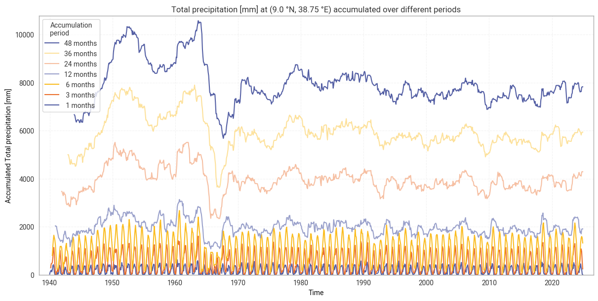
Fig. 6.1.1 Total precipitation from ERA5 accumulated over different periods, for the example site of Addis Ababa, Ethiopia.

3.3 Fit gamma distribution by calendar month

At the core of SPI is the assumption that (monthly) total precipitation values follow a gamma distribution. Here, this distribution is fitted to data within the reference period (1991–2020 by default, see above). A separate distribution is fitted for each calendar month, i.e. we fit one distribution for all 30 Januaries in the reference period, another for all 30 Februaries, and so on. This separation allows the resulting index to account for seasonal differences. This fitting process is then repeated for each accumulation period.

Here, we use scipy.stats.gamma to fit the gamma distribution. This returns three parameters for each calendar month and accumulation period, namely shape (α), location (μ), and scale (β).

Show code cell source

Hide code cell source

# Select data in reference window
data_era5_precipitation_reference = data_era5_precipitation.sel(**reference_window)

# Fit gamma distribution
spi_parameters = fit_monthly_spi(data_era5_precipitation_reference)

# Display result
spi_parameters

Show code cell output

Hide code cell output

<xarray.Dataset> Size: 2GB
Dimensions:  (month: 12, lat: 721, lon: 1440, stat: 3)
Coordinates:
    number   int64 8B ...
  * lat      (lat) float64 6kB 90.0 89.75 89.5 89.25 ... -89.5 -89.75 -90.0
  * lon      (lon) float64 12kB -180.0 -179.8 -179.5 ... 179.2 179.5 179.8
  * month    (month) int64 96B 1 2 3 4 5 6 7 8 9 10 11 12
Dimensions without coordinates: stat
Data variables:
    tp1      (month, lat, lon, stat) float64 299MB dask.array<chunksize=(12, 103, 360, 3), meta=np.ndarray>
    tp3      (month, lat, lon, stat) float64 299MB dask.array<chunksize=(12, 103, 360, 3), meta=np.ndarray>
    tp6      (month, lat, lon, stat) float64 299MB dask.array<chunksize=(12, 103, 360, 3), meta=np.ndarray>
    tp12     (month, lat, lon, stat) float64 299MB dask.array<chunksize=(12, 103, 360, 3), meta=np.ndarray>
    tp24     (month, lat, lon, stat) float64 299MB dask.array<chunksize=(12, 103, 360, 3), meta=np.ndarray>
    tp36     (month, lat, lon, stat) float64 299MB dask.array<chunksize=(12, 103, 360, 3), meta=np.ndarray>
    tp48     (month, lat, lon, stat) float64 299MB dask.array<chunksize=(12, 103, 360, 3), meta=np.ndarray>

xarray.Dataset

• Dimensions:
  • month: 12
  • lat: 721
  • lon: 1440
  • stat: 3
• Coordinates: (4)
  • number
    ()
    int64
    ...

    long_name :

    ensemble member numerical id

    units :

    1

    standard_name :

    realization

    [1 values with dtype=int64]

  • lat
    (lat)
    float64
    90.0 89.75 89.5 ... -89.75 -90.0

    units :

    degrees_north

    standard_name :

    latitude

    long_name :

    latitude

    stored_direction :

    decreasing

    array([ 90.  ,  89.75,  89.5 , ..., -89.5 , -89.75, -90.  ], shape=(721,))

  • lon
    (lon)
    float64
    -180.0 -179.8 ... 179.5 179.8

    array([-180.  , -179.75, -179.5 , ...,  179.25,  179.5 ,  179.75],
          shape=(1440,))

  • month
    (month)
    int64
    1 2 3 4 5 6 7 8 9 10 11 12

    long_name :

    time

    standard_name :

    time

    array([ 1,  2,  3,  4,  5,  6,  7,  8,  9, 10, 11, 12])

• Data variables: (7)
  • tp1
    (month, lat, lon, stat)
    float64
    dask.array<chunksize=(12, 103, 360, 3), meta=np.ndarray>

    Array Chunk Bytes 285.16 MiB 10.18 MiB Shape (12, 721, 1440, 3) (12, 103, 360, 3) Dask graph 28 chunks in 95 graph layers Data type float64 numpy.ndarray

  • tp3
    (month, lat, lon, stat)
    float64
    dask.array<chunksize=(12, 103, 360, 3), meta=np.ndarray>

    Array Chunk Bytes 285.16 MiB 10.18 MiB Shape (12, 721, 1440, 3) (12, 103, 360, 3) Dask graph 28 chunks in 105 graph layers Data type float64 numpy.ndarray

  • tp6
    (month, lat, lon, stat)
    float64
    dask.array<chunksize=(12, 103, 360, 3), meta=np.ndarray>

    Array Chunk Bytes 285.16 MiB 10.18 MiB Shape (12, 721, 1440, 3) (12, 103, 360, 3) Dask graph 28 chunks in 105 graph layers Data type float64 numpy.ndarray

  • tp12
    (month, lat, lon, stat)
    float64
    dask.array<chunksize=(12, 103, 360, 3), meta=np.ndarray>

    Array Chunk Bytes 285.16 MiB 10.18 MiB Shape (12, 721, 1440, 3) (12, 103, 360, 3) Dask graph 28 chunks in 105 graph layers Data type float64 numpy.ndarray

  • tp24
    (month, lat, lon, stat)
    float64
    dask.array<chunksize=(12, 103, 360, 3), meta=np.ndarray>

    Array Chunk Bytes 285.16 MiB 10.18 MiB Shape (12, 721, 1440, 3) (12, 103, 360, 3) Dask graph 28 chunks in 105 graph layers Data type float64 numpy.ndarray

  • tp36
    (month, lat, lon, stat)
    float64
    dask.array<chunksize=(12, 103, 360, 3), meta=np.ndarray>

    Array Chunk Bytes 285.16 MiB 10.18 MiB Shape (12, 721, 1440, 3) (12, 103, 360, 3) Dask graph 28 chunks in 105 graph layers Data type float64 numpy.ndarray

  • tp48
    (month, lat, lon, stat)
    float64
    dask.array<chunksize=(12, 103, 360, 3), meta=np.ndarray>

    Array Chunk Bytes 285.16 MiB 10.18 MiB Shape (12, 721, 1440, 3) (12, 103, 360, 3) Dask graph 28 chunks in 105 graph layers Data type float64 numpy.ndarray

• Indexes: (3)
  • lat
    PandasIndex

    PandasIndex(Index([  90.0,  89.75,   89.5,  89.25,   89.0,  88.75,   88.5,  88.25,   88.0,
            87.75,
           ...
           -87.75,  -88.0, -88.25,  -88.5, -88.75,  -89.0, -89.25,  -89.5, -89.75,
            -90.0],
          dtype='float64', name='lat', length=721))

  • lon
    PandasIndex

    PandasIndex(Index([ -180.0, -179.75,  -179.5, -179.25,  -179.0, -178.75,  -178.5, -178.25,
            -178.0, -177.75,
           ...
             177.5,  177.75,   178.0,  178.25,   178.5,  178.75,   179.0,  179.25,
             179.5,  179.75],
          dtype='float64', name='lon', length=1440))

  • month
    PandasIndex

    PandasIndex(Index([1, 2, 3, 4, 5, 6, 7, 8, 9, 10, 11, 12], dtype='int64', name='month'))

• Attributes: (0)

The observed (accumulated) total precipitation values along the entire time series (1940–2024 in our example) are then compared to the fitted parameters. This is quantified in terms of where the observed values fall on the cumulative distribution function (CDF):

\[ P(X \leq x) = F_X(x ; \alpha, \mu, \beta) = \int_{-\infty}^{x}f(y ; \alpha, \mu, \beta) \, \text{d}y \]

Where P(X ≤ x) is the probability for a randomly drawn total precipitation X to be equal to or less than the observed value x; F_X is the CDF for a gamma distribution with shape α, location µ, and scale β; and the CDF is equal to the integral of the corresponding probability density function up to x.

As before, there is a distribution for each calendar month, for each accumulation period.

Note that actually evaluating the CDF – as opposed to queueing it up in dask, as done here – can be slow, especially for a large dataset like global ERA5 precipitation. As such, if you are interested in a subset of the data, such as a specific site or period in time, it may be best to subset your data before calculating the CDF rather than afterwards. An example of this is provided below in the comparison with ERA5–Drought SPI.

Show code cell source

Hide code cell source

# Compute CDF time series
cdf = compute_cdf_spi(data_era5_precipitation, spi_parameters)

# Display result
cdf

Show code cell output

Hide code cell output

<xarray.Dataset> Size: 59GB
Dimensions:  (time: 1020, lat: 721, lon: 1440)
Coordinates:
    number   int64 8B 0
  * time     (time) datetime64[ns] 8kB 1940-01-01T06:00:00 ... 2024-12-01T06:...
  * lat      (lat) float64 6kB 90.0 89.75 89.5 89.25 ... -89.5 -89.75 -90.0
    expver   (time) <U4 16kB dask.array<chunksize=(1020,), meta=np.ndarray>
  * lon      (lon) float64 12kB -180.0 -179.8 -179.5 ... 179.2 179.5 179.8
    month    (time) int64 8kB dask.array<chunksize=(1020,), meta=np.ndarray>
Data variables:
    tp1      (time, lat, lon) float64 8GB dask.array<chunksize=(1020, 103, 360), meta=np.ndarray>
    tp3      (time, lat, lon) float64 8GB dask.array<chunksize=(1020, 103, 360), meta=np.ndarray>
    tp6      (time, lat, lon) float64 8GB dask.array<chunksize=(1020, 103, 360), meta=np.ndarray>
    tp12     (time, lat, lon) float64 8GB dask.array<chunksize=(1020, 103, 360), meta=np.ndarray>
    tp24     (time, lat, lon) float64 8GB dask.array<chunksize=(1020, 103, 360), meta=np.ndarray>
    tp36     (time, lat, lon) float64 8GB dask.array<chunksize=(1020, 103, 360), meta=np.ndarray>
    tp48     (time, lat, lon) float64 8GB dask.array<chunksize=(1020, 103, 360), meta=np.ndarray>
Attributes:
    GRIB_centre:             ecmf
    GRIB_centreDescription:  European Centre for Medium-Range Weather Forecasts
    GRIB_subCentre:          0
    Conventions:             CF-1.7
    institution:             European Centre for Medium-Range Weather Forecasts

xarray.Dataset

• Dimensions:
  • time: 1020
  • lat: 721
  • lon: 1440
• Coordinates: (6)
  • number
    ()
    int64
    0

    long_name :

    ensemble member numerical id

    units :

    1

    standard_name :

    realization

    array(0)

  • time
    (time)
    datetime64[ns]
    1940-01-01T06:00:00 ... 2024-12-...

    long_name :

    time

    standard_name :

    time

    array(['1940-01-01T06:00:00.000000000', '1940-02-01T06:00:00.000000000',
           '1940-03-01T06:00:00.000000000', ..., '2024-10-01T06:00:00.000000000',
           '2024-11-01T06:00:00.000000000', '2024-12-01T06:00:00.000000000'],
          shape=(1020,), dtype='datetime64[ns]')

  • lat
    (lat)
    float64
    90.0 89.75 89.5 ... -89.75 -90.0

    units :

    degrees_north

    standard_name :

    latitude

    long_name :

    latitude

    stored_direction :

    decreasing

    array([ 90.  ,  89.75,  89.5 , ..., -89.5 , -89.75, -90.  ], shape=(721,))

  • expver
    (time)
    <U4
    dask.array<chunksize=(1020,), meta=np.ndarray>

    Array Chunk Bytes 15.94 kiB 15.94 kiB Shape (1020,) (1020,) Dask graph 1 chunks in 2 graph layers Data type

  • lon
    (lon)
    float64
    -180.0 -179.8 ... 179.5 179.8

    array([-180.  , -179.75, -179.5 , ...,  179.25,  179.5 ,  179.75],
          shape=(1440,))

  • month
    (time)
    int64
    dask.array<chunksize=(1020,), meta=np.ndarray>

    long_name :

    time

    standard_name :

    time

    Array Chunk Bytes 7.97 kiB 7.97 kiB Shape (1020,) (1020,) Dask graph 1 chunks in 1 graph layer Data type int64 numpy.ndarray

• Data variables: (7)
  • tp1
    (time, lat, lon)
    float64
    dask.array<chunksize=(1020, 103, 360), meta=np.ndarray>

    Array Chunk Bytes 7.89 GiB 288.56 MiB Shape (1020, 721, 1440) (1020, 103, 360) Dask graph 28 chunks in 107 graph layers Data type float64 numpy.ndarray

  • tp3
    (time, lat, lon)
    float64
    dask.array<chunksize=(1020, 103, 360), meta=np.ndarray>

    Array Chunk Bytes 7.89 GiB 288.56 MiB Shape (1020, 721, 1440) (1020, 103, 360) Dask graph 28 chunks in 117 graph layers Data type float64 numpy.ndarray

  • tp6
    (time, lat, lon)
    float64
    dask.array<chunksize=(1020, 103, 360), meta=np.ndarray>

    Array Chunk Bytes 7.89 GiB 288.56 MiB Shape (1020, 721, 1440) (1020, 103, 360) Dask graph 28 chunks in 117 graph layers Data type float64 numpy.ndarray

  • tp12
    (time, lat, lon)
    float64
    dask.array<chunksize=(1020, 103, 360), meta=np.ndarray>

    Array Chunk Bytes 7.89 GiB 288.56 MiB Shape (1020, 721, 1440) (1020, 103, 360) Dask graph 28 chunks in 117 graph layers Data type float64 numpy.ndarray

  • tp24
    (time, lat, lon)
    float64
    dask.array<chunksize=(1020, 103, 360), meta=np.ndarray>

    Array Chunk Bytes 7.89 GiB 288.56 MiB Shape (1020, 721, 1440) (1020, 103, 360) Dask graph 28 chunks in 117 graph layers Data type float64 numpy.ndarray

  • tp36
    (time, lat, lon)
    float64
    dask.array<chunksize=(1020, 103, 360), meta=np.ndarray>

    Array Chunk Bytes 7.89 GiB 288.56 MiB Shape (1020, 721, 1440) (1020, 103, 360) Dask graph 28 chunks in 117 graph layers Data type float64 numpy.ndarray

  • tp48
    (time, lat, lon)
    float64
    dask.array<chunksize=(1020, 103, 360), meta=np.ndarray>

    Array Chunk Bytes 7.89 GiB 288.56 MiB Shape (1020, 721, 1440) (1020, 103, 360) Dask graph 28 chunks in 117 graph layers Data type float64 numpy.ndarray

• Indexes: (3)
  • time
    PandasIndex

    PandasIndex(DatetimeIndex(['1940-01-01 06:00:00', '1940-02-01 06:00:00',
                   '1940-03-01 06:00:00', '1940-04-01 06:00:00',
                   '1940-05-01 06:00:00', '1940-06-01 06:00:00',
                   '1940-07-01 06:00:00', '1940-08-01 06:00:00',
                   '1940-09-01 06:00:00', '1940-10-01 06:00:00',
                   ...
                   '2024-03-01 06:00:00', '2024-04-01 06:00:00',
                   '2024-05-01 06:00:00', '2024-06-01 06:00:00',
                   '2024-07-01 06:00:00', '2024-08-01 06:00:00',
                   '2024-09-01 06:00:00', '2024-10-01 06:00:00',
                   '2024-11-01 06:00:00', '2024-12-01 06:00:00'],
                  dtype='datetime64[ns]', name='time', length=1020, freq=None))

  • lat
    PandasIndex

    PandasIndex(Index([  90.0,  89.75,   89.5,  89.25,   89.0,  88.75,   88.5,  88.25,   88.0,
            87.75,
           ...
           -87.75,  -88.0, -88.25,  -88.5, -88.75,  -89.0, -89.25,  -89.5, -89.75,
            -90.0],
          dtype='float64', name='lat', length=721))

  • lon
    PandasIndex

    PandasIndex(Index([ -180.0, -179.75,  -179.5, -179.25,  -179.0, -178.75,  -178.5, -178.25,
            -178.0, -177.75,
           ...
             177.5,  177.75,   178.0,  178.25,   178.5,  178.75,   179.0,  179.25,
             179.5,  179.75],
          dtype='float64', name='lon', length=1440))

• Attributes: (5)

  GRIB_centre :

  ecmf

  GRIB_centreDescription :

  European Centre for Medium-Range Weather Forecasts

  GRIB_subCentre :

  0

  Conventions :

  CF-1.7

  institution :

  European Centre for Medium-Range Weather Forecasts

3.4 Adjust for months with zero precipitation

Sometimes, zero (or near-zero) monthly precipitation is observed, particularly in dry areas like deserts. Maintaining the desired statistics, such as the mean SPI in the reference period being 0, requires adjusting the CDF to account for these zero-precipitation months.

ERA5–Drought follows the [Stagge+15] method to adjust the CDF. First, the probability of zero precipitation is calculated as follows:

\[ \bar{p_0} = \frac{n_0 + 1}{2 (n + 1)} \]

where n₀ is the number of months with zero precipitation in the reference period, and n is the total number of months in the reference period (here 30 for 1991–2020). While some datasets define “zero precipitation” using a slightly higher threshold (e.g. less than 0.1 mm) to account for measurement uncertainty, ERA5–Drought uses a threshold of exactly 0 mm total precipitation in the underpinning ERA5 data.

Having calculated the probability of zero precipitation, the CDF is adjusted as follows:

\[\begin{split} F'_X(x ; \alpha, \mu, \beta) = \begin{cases} \bar{p_0} + (1 - \bar{p_0}) \, F_X(x; \alpha, \mu, \beta), & x > 0, \\ \frac{n_0 + 1}{2(n+1)}, & x = 0 \end{cases} \end{split}\]

As before, this adjustment is carried out individually for each calendar month and accumulation period.

Show code cell source

Hide code cell source

# Adjust CDF
cdf_adjusted = adjust_cdf_for_zero_precipitation(cdf, data_era5_precipitation_reference)

# Display result
cdf_adjusted

Show code cell output

Hide code cell output

<xarray.Dataset> Size: 59GB
Dimensions:  (lat: 721, lon: 1440, time: 1020)
Coordinates:
    number   int64 8B 0
  * lat      (lat) float64 6kB 90.0 89.75 89.5 89.25 ... -89.5 -89.75 -90.0
  * lon      (lon) float64 12kB -180.0 -179.8 -179.5 ... 179.2 179.5 179.8
    month    (time) int64 8kB dask.array<chunksize=(1020,), meta=np.ndarray>
  * time     (time) datetime64[ns] 8kB 1940-01-01T06:00:00 ... 2024-12-01T06:...
    expver   (time) <U4 16kB dask.array<chunksize=(1020,), meta=np.ndarray>
Data variables:
    tp1      (lat, lon, time) float64 8GB dask.array<chunksize=(103, 360, 1020), meta=np.ndarray>
    tp3      (lat, lon, time) float64 8GB dask.array<chunksize=(103, 360, 1020), meta=np.ndarray>
    tp6      (lat, lon, time) float64 8GB dask.array<chunksize=(103, 360, 1020), meta=np.ndarray>
    tp12     (lat, lon, time) float64 8GB dask.array<chunksize=(103, 360, 1020), meta=np.ndarray>
    tp24     (lat, lon, time) float64 8GB dask.array<chunksize=(103, 360, 1020), meta=np.ndarray>
    tp36     (lat, lon, time) float64 8GB dask.array<chunksize=(103, 360, 1020), meta=np.ndarray>
    tp48     (lat, lon, time) float64 8GB dask.array<chunksize=(103, 360, 1020), meta=np.ndarray>

xarray.Dataset

• Dimensions:
  • lat: 721
  • lon: 1440
  • time: 1020
• Coordinates: (6)
  • number
    ()
    int64
    0

    array(0)

  • lat
    (lat)
    float64
    90.0 89.75 89.5 ... -89.75 -90.0

    array([ 90.  ,  89.75,  89.5 , ..., -89.5 , -89.75, -90.  ], shape=(721,))

  • lon
    (lon)
    float64
    -180.0 -179.8 ... 179.5 179.8

    array([-180.  , -179.75, -179.5 , ...,  179.25,  179.5 ,  179.75],
          shape=(1440,))

  • month
    (time)
    int64
    dask.array<chunksize=(1020,), meta=np.ndarray>

    Array Chunk Bytes 7.97 kiB 7.97 kiB Shape (1020,) (1020,) Dask graph 1 chunks in 1 graph layer Data type int64 numpy.ndarray

  • time
    (time)
    datetime64[ns]
    1940-01-01T06:00:00 ... 2024-12-...

    long_name :

    time

    standard_name :

    time

    array(['1940-01-01T06:00:00.000000000', '1940-02-01T06:00:00.000000000',
           '1940-03-01T06:00:00.000000000', ..., '2024-10-01T06:00:00.000000000',
           '2024-11-01T06:00:00.000000000', '2024-12-01T06:00:00.000000000'],
          shape=(1020,), dtype='datetime64[ns]')

  • expver
    (time)
    <U4
    dask.array<chunksize=(1020,), meta=np.ndarray>

    Array Chunk Bytes 15.94 kiB 15.94 kiB Shape (1020,) (1020,) Dask graph 1 chunks in 29 graph layers Data type

• Data variables: (7)
  • tp1
    (lat, lon, time)
    float64
    dask.array<chunksize=(103, 360, 1020), meta=np.ndarray>

    Array Chunk Bytes 7.89 GiB 288.56 MiB Shape (721, 1440, 1020) (103, 360, 1020) Dask graph 28 chunks in 296 graph layers Data type float64 numpy.ndarray

  • tp3
    (lat, lon, time)
    float64
    dask.array<chunksize=(103, 360, 1020), meta=np.ndarray>

    Array Chunk Bytes 7.89 GiB 288.56 MiB Shape (721, 1440, 1020) (103, 360, 1020) Dask graph 28 chunks in 306 graph layers Data type float64 numpy.ndarray

  • tp6
    (lat, lon, time)
    float64
    dask.array<chunksize=(103, 360, 1020), meta=np.ndarray>

    Array Chunk Bytes 7.89 GiB 288.56 MiB Shape (721, 1440, 1020) (103, 360, 1020) Dask graph 28 chunks in 306 graph layers Data type float64 numpy.ndarray

  • tp12
    (lat, lon, time)
    float64
    dask.array<chunksize=(103, 360, 1020), meta=np.ndarray>

    Array Chunk Bytes 7.89 GiB 288.56 MiB Shape (721, 1440, 1020) (103, 360, 1020) Dask graph 28 chunks in 306 graph layers Data type float64 numpy.ndarray

  • tp24
    (lat, lon, time)
    float64
    dask.array<chunksize=(103, 360, 1020), meta=np.ndarray>

    Array Chunk Bytes 7.89 GiB 288.56 MiB Shape (721, 1440, 1020) (103, 360, 1020) Dask graph 28 chunks in 306 graph layers Data type float64 numpy.ndarray

  • tp36
    (lat, lon, time)
    float64
    dask.array<chunksize=(103, 360, 1020), meta=np.ndarray>

    Array Chunk Bytes 7.89 GiB 288.56 MiB Shape (721, 1440, 1020) (103, 360, 1020) Dask graph 28 chunks in 306 graph layers Data type float64 numpy.ndarray

  • tp48
    (lat, lon, time)
    float64
    dask.array<chunksize=(103, 360, 1020), meta=np.ndarray>

    Array Chunk Bytes 7.89 GiB 288.56 MiB Shape (721, 1440, 1020) (103, 360, 1020) Dask graph 28 chunks in 306 graph layers Data type float64 numpy.ndarray

• Indexes: (3)
  • lat
    PandasIndex

    PandasIndex(Index([  90.0,  89.75,   89.5,  89.25,   89.0,  88.75,   88.5,  88.25,   88.0,
            87.75,
           ...
           -87.75,  -88.0, -88.25,  -88.5, -88.75,  -89.0, -89.25,  -89.5, -89.75,
            -90.0],
          dtype='float64', name='lat', length=721))

  • lon
    PandasIndex

    PandasIndex(Index([ -180.0, -179.75,  -179.5, -179.25,  -179.0, -178.75,  -178.5, -178.25,
            -178.0, -177.75,
           ...
             177.5,  177.75,   178.0,  178.25,   178.5,  178.75,   179.0,  179.25,
             179.5,  179.75],
          dtype='float64', name='lon', length=1440))

  • time
    PandasIndex

    PandasIndex(DatetimeIndex(['1940-01-01 06:00:00', '1940-02-01 06:00:00',
                   '1940-03-01 06:00:00', '1940-04-01 06:00:00',
                   '1940-05-01 06:00:00', '1940-06-01 06:00:00',
                   '1940-07-01 06:00:00', '1940-08-01 06:00:00',
                   '1940-09-01 06:00:00', '1940-10-01 06:00:00',
                   ...
                   '2024-03-01 06:00:00', '2024-04-01 06:00:00',
                   '2024-05-01 06:00:00', '2024-06-01 06:00:00',
                   '2024-07-01 06:00:00', '2024-08-01 06:00:00',
                   '2024-09-01 06:00:00', '2024-10-01 06:00:00',
                   '2024-11-01 06:00:00', '2024-12-01 06:00:00'],
                  dtype='datetime64[ns]', name='time', length=1020, freq=None))

• Attributes: (0)

3.5 Compute SPI

Finally, SPI values for each data point (latitude, longitude, time) are calculated from the adjusted CDF values F’_X by transforming to a standard normal distribution. The function scipy.stats.norm.ppf is used to calculate the inverse CDF Φ^-1 of the normal distribution:

\[ \text{SPI}(x) = \Phi^{-1}\left(F'_X(x ; \alpha, \mu, \beta)\right) \]

Show code cell source

Hide code cell source

# Calculate SPI from adjusted CDF
spi_reproduced = cdf_to_spi(cdf_adjusted)

# Display result
spi_reproduced

<xarray.Dataset> Size: 59GB
Dimensions:  (lat: 721, lon: 1440, time: 1020)
Coordinates:
    number   int64 8B 0
  * lat      (lat) float64 6kB 90.0 89.75 89.5 89.25 ... -89.5 -89.75 -90.0
  * lon      (lon) float64 12kB -180.0 -179.8 -179.5 ... 179.2 179.5 179.8
    month    (time) int64 8kB dask.array<chunksize=(1020,), meta=np.ndarray>
  * time     (time) datetime64[ns] 8kB 1940-01-01T06:00:00 ... 2024-12-01T06:...
    expver   (time) <U4 16kB dask.array<chunksize=(1020,), meta=np.ndarray>
Data variables:
    SPI1     (lat, lon, time) float64 8GB dask.array<chunksize=(103, 360, 1020), meta=np.ndarray>
    SPI3     (lat, lon, time) float64 8GB dask.array<chunksize=(103, 360, 1020), meta=np.ndarray>
    SPI6     (lat, lon, time) float64 8GB dask.array<chunksize=(103, 360, 1020), meta=np.ndarray>
    SPI12    (lat, lon, time) float64 8GB dask.array<chunksize=(103, 360, 1020), meta=np.ndarray>
    SPI24    (lat, lon, time) float64 8GB dask.array<chunksize=(103, 360, 1020), meta=np.ndarray>
    SPI36    (lat, lon, time) float64 8GB dask.array<chunksize=(103, 360, 1020), meta=np.ndarray>
    SPI48    (lat, lon, time) float64 8GB dask.array<chunksize=(103, 360, 1020), meta=np.ndarray>

xarray.Dataset

• Dimensions:
  • lat: 721
  • lon: 1440
  • time: 1020
• Coordinates: (6)
  • number
    ()
    int64
    0

    array(0)

  • lat
    (lat)
    float64
    90.0 89.75 89.5 ... -89.75 -90.0

    array([ 90.  ,  89.75,  89.5 , ..., -89.5 , -89.75, -90.  ], shape=(721,))

  • lon
    (lon)
    float64
    -180.0 -179.8 ... 179.5 179.8

    array([-180.  , -179.75, -179.5 , ...,  179.25,  179.5 ,  179.75],
          shape=(1440,))

  • month
    (time)
    int64
    dask.array<chunksize=(1020,), meta=np.ndarray>

    Array Chunk Bytes 7.97 kiB 7.97 kiB Shape (1020,) (1020,) Dask graph 1 chunks in 1 graph layer Data type int64 numpy.ndarray

  • time
    (time)
    datetime64[ns]
    1940-01-01T06:00:00 ... 2024-12-...

    long_name :

    time

    standard_name :

    time

    array(['1940-01-01T06:00:00.000000000', '1940-02-01T06:00:00.000000000',
           '1940-03-01T06:00:00.000000000', ..., '2024-10-01T06:00:00.000000000',
           '2024-11-01T06:00:00.000000000', '2024-12-01T06:00:00.000000000'],
          shape=(1020,), dtype='datetime64[ns]')

  • expver
    (time)
    <U4
    dask.array<chunksize=(1020,), meta=np.ndarray>

    Array Chunk Bytes 15.94 kiB 15.94 kiB Shape (1020,) (1020,) Dask graph 1 chunks in 29 graph layers Data type

• Data variables: (7)
  • SPI1
    (lat, lon, time)
    float64
    dask.array<chunksize=(103, 360, 1020), meta=np.ndarray>

    Array Chunk Bytes 7.89 GiB 288.56 MiB Shape (721, 1440, 1020) (103, 360, 1020) Dask graph 28 chunks in 302 graph layers Data type float64 numpy.ndarray

  • SPI3
    (lat, lon, time)
    float64
    dask.array<chunksize=(103, 360, 1020), meta=np.ndarray>

    Array Chunk Bytes 7.89 GiB 288.56 MiB Shape (721, 1440, 1020) (103, 360, 1020) Dask graph 28 chunks in 311 graph layers Data type float64 numpy.ndarray

  • SPI6
    (lat, lon, time)
    float64
    dask.array<chunksize=(103, 360, 1020), meta=np.ndarray>

    Array Chunk Bytes 7.89 GiB 288.56 MiB Shape (721, 1440, 1020) (103, 360, 1020) Dask graph 28 chunks in 311 graph layers Data type float64 numpy.ndarray

  • SPI12
    (lat, lon, time)
    float64
    dask.array<chunksize=(103, 360, 1020), meta=np.ndarray>

    Array Chunk Bytes 7.89 GiB 288.56 MiB Shape (721, 1440, 1020) (103, 360, 1020) Dask graph 28 chunks in 311 graph layers Data type float64 numpy.ndarray

  • SPI24
    (lat, lon, time)
    float64
    dask.array<chunksize=(103, 360, 1020), meta=np.ndarray>

    Array Chunk Bytes 7.89 GiB 288.56 MiB Shape (721, 1440, 1020) (103, 360, 1020) Dask graph 28 chunks in 311 graph layers Data type float64 numpy.ndarray

  • SPI36
    (lat, lon, time)
    float64
    dask.array<chunksize=(103, 360, 1020), meta=np.ndarray>

    Array Chunk Bytes 7.89 GiB 288.56 MiB Shape (721, 1440, 1020) (103, 360, 1020) Dask graph 28 chunks in 311 graph layers Data type float64 numpy.ndarray

  • SPI48
    (lat, lon, time)
    float64
    dask.array<chunksize=(103, 360, 1020), meta=np.ndarray>

    Array Chunk Bytes 7.89 GiB 288.56 MiB Shape (721, 1440, 1020) (103, 360, 1020) Dask graph 28 chunks in 311 graph layers Data type float64 numpy.ndarray

• Indexes: (3)
  • lat
    PandasIndex

    PandasIndex(Index([  90.0,  89.75,   89.5,  89.25,   89.0,  88.75,   88.5,  88.25,   88.0,
            87.75,
           ...
           -87.75,  -88.0, -88.25,  -88.5, -88.75,  -89.0, -89.25,  -89.5, -89.75,
            -90.0],
          dtype='float64', name='lat', length=721))

  • lon
    PandasIndex

    PandasIndex(Index([ -180.0, -179.75,  -179.5, -179.25,  -179.0, -178.75,  -178.5, -178.25,
            -178.0, -177.75,
           ...
             177.5,  177.75,   178.0,  178.25,   178.5,  178.75,   179.0,  179.25,
             179.5,  179.75],
          dtype='float64', name='lon', length=1440))

  • time
    PandasIndex

    PandasIndex(DatetimeIndex(['1940-01-01 06:00:00', '1940-02-01 06:00:00',
                   '1940-03-01 06:00:00', '1940-04-01 06:00:00',
                   '1940-05-01 06:00:00', '1940-06-01 06:00:00',
                   '1940-07-01 06:00:00', '1940-08-01 06:00:00',
                   '1940-09-01 06:00:00', '1940-10-01 06:00:00',
                   ...
                   '2024-03-01 06:00:00', '2024-04-01 06:00:00',
                   '2024-05-01 06:00:00', '2024-06-01 06:00:00',
                   '2024-07-01 06:00:00', '2024-08-01 06:00:00',
                   '2024-09-01 06:00:00', '2024-10-01 06:00:00',
                   '2024-11-01 06:00:00', '2024-12-01 06:00:00'],
                  dtype='datetime64[ns]', name='time', length=1020, freq=None))

• Attributes: (0)

3.6 SPI comparison: Time series in example site

Having reproduced the SPI index from ERA5 precipitation data following the ERA5–Drought methodology, we can now compare the results to determine the reproducibility of ERA5–Drought. We first compare the datasets over time at the example site defined in 2. General setup.

The previous sections set up the SPI reproduction pipeline for the entire ERA5 precipitation dataset (global, 1940–2024). Because actually executing said calculation takes a long time, as noted in the CDF subsection, here we sub-select the downloaded ERA5 precipitation data and calculate SPI for the example site only. For convenience, the full SPI pipeline is wrapped into a single calculate_spi_from_era5 function, as defined in 1. Code setup.

Note that while the two may seem equivalent, downloading the ERA5 precipitation data for the example site only and then running the SPI pipeline, rather than downloading the entire dataset and subselecting for the example site, produces different results. This is likely caused by the inner workings of the MARS regridding function. For consistency with ERA5–Drought, it is necessary to download the global ERA5 dataset and subselect.

Show code cell source

Hide code cell source

# Select only desired site
data_era5_precipitation_site = data_era5_precipitation_preprocessed.sel(**example_site)

# Calculate SPI
spi_reproduced_site = calculate_spi_from_era5(data_era5_precipitation_site, reference_window=reference_window)

# Persist in memory to speed up analysis – this step may take a few minutes
spi_reproduced_site = spi_reproduced_site.persist()

# Display result
spi_reproduced_site

Show code cell output

Hide code cell output

<xarray.Dataset> Size: 90kB
Dimensions:  (time: 1020)
Coordinates:
    number   int64 8B 0
    lat      float64 8B 9.0
    lon      float64 8B 38.75
    month    (time) int64 8kB dask.array<chunksize=(1020,), meta=np.ndarray>
  * time     (time) datetime64[ns] 8kB 1940-01-01T06:00:00 ... 2024-12-01T06:...
    expver   (time) <U4 16kB dask.array<chunksize=(1020,), meta=np.ndarray>
Data variables:
    SPI1     (time) float64 8kB dask.array<chunksize=(1020,), meta=np.ndarray>
    SPI3     (time) float64 8kB dask.array<chunksize=(1020,), meta=np.ndarray>
    SPI6     (time) float64 8kB dask.array<chunksize=(1020,), meta=np.ndarray>
    SPI12    (time) float64 8kB dask.array<chunksize=(1020,), meta=np.ndarray>
    SPI24    (time) float64 8kB dask.array<chunksize=(1020,), meta=np.ndarray>
    SPI36    (time) float64 8kB dask.array<chunksize=(1020,), meta=np.ndarray>
    SPI48    (time) float64 8kB dask.array<chunksize=(1020,), meta=np.ndarray>

xarray.Dataset

• Dimensions:
  • time: 1020
• Coordinates: (6)
  • number
    ()
    int64
    0

    array(0)

  • lat
    ()
    float64
    9.0

    array(9.)

  • lon
    ()
    float64
    38.75

    array(38.75)

  • month
    (time)
    int64
    dask.array<chunksize=(1020,), meta=np.ndarray>

    Array Chunk Bytes 7.97 kiB 7.97 kiB Shape (1020,) (1020,) Dask graph 1 chunks in 1 graph layer Data type int64 numpy.ndarray

  • time
    (time)
    datetime64[ns]
    1940-01-01T06:00:00 ... 2024-12-...

    long_name :

    time

    standard_name :

    time

    array(['1940-01-01T06:00:00.000000000', '1940-02-01T06:00:00.000000000',
           '1940-03-01T06:00:00.000000000', ..., '2024-10-01T06:00:00.000000000',
           '2024-11-01T06:00:00.000000000', '2024-12-01T06:00:00.000000000'],
          shape=(1020,), dtype='datetime64[ns]')

  • expver
    (time)
    <U4
    dask.array<chunksize=(1020,), meta=np.ndarray>

    Array Chunk Bytes 15.94 kiB 15.94 kiB Shape (1020,) (1020,) Dask graph 1 chunks in 1 graph layer Data type

• Data variables: (7)
  • SPI1
    (time)
    float64
    dask.array<chunksize=(1020,), meta=np.ndarray>

    Array Chunk Bytes 7.97 kiB 7.97 kiB Shape (1020,) (1020,) Dask graph 1 chunks in 1 graph layer Data type float64 numpy.ndarray

  • SPI3
    (time)
    float64
    dask.array<chunksize=(1020,), meta=np.ndarray>

    Array Chunk Bytes 7.97 kiB 7.97 kiB Shape (1020,) (1020,) Dask graph 1 chunks in 1 graph layer Data type float64 numpy.ndarray

  • SPI6
    (time)
    float64
    dask.array<chunksize=(1020,), meta=np.ndarray>

    Array Chunk Bytes 7.97 kiB 7.97 kiB Shape (1020,) (1020,) Dask graph 1 chunks in 1 graph layer Data type float64 numpy.ndarray

  • SPI12
    (time)
    float64
    dask.array<chunksize=(1020,), meta=np.ndarray>

    Array Chunk Bytes 7.97 kiB 7.97 kiB Shape (1020,) (1020,) Dask graph 1 chunks in 1 graph layer Data type float64 numpy.ndarray

  • SPI24
    (time)
    float64
    dask.array<chunksize=(1020,), meta=np.ndarray>

    Array Chunk Bytes 7.97 kiB 7.97 kiB Shape (1020,) (1020,) Dask graph 1 chunks in 1 graph layer Data type float64 numpy.ndarray

  • SPI36
    (time)
    float64
    dask.array<chunksize=(1020,), meta=np.ndarray>

    Array Chunk Bytes 7.97 kiB 7.97 kiB Shape (1020,) (1020,) Dask graph 1 chunks in 1 graph layer Data type float64 numpy.ndarray

  • SPI48
    (time)
    float64
    dask.array<chunksize=(1020,), meta=np.ndarray>

    Array Chunk Bytes 7.97 kiB 7.97 kiB Shape (1020,) (1020,) Dask graph 1 chunks in 1 graph layer Data type float64 numpy.ndarray

• Indexes: (1)
  • time
    PandasIndex

    PandasIndex(DatetimeIndex(['1940-01-01 06:00:00', '1940-02-01 06:00:00',
                   '1940-03-01 06:00:00', '1940-04-01 06:00:00',
                   '1940-05-01 06:00:00', '1940-06-01 06:00:00',
                   '1940-07-01 06:00:00', '1940-08-01 06:00:00',
                   '1940-09-01 06:00:00', '1940-10-01 06:00:00',
                   ...
                   '2024-03-01 06:00:00', '2024-04-01 06:00:00',
                   '2024-05-01 06:00:00', '2024-06-01 06:00:00',
                   '2024-07-01 06:00:00', '2024-08-01 06:00:00',
                   '2024-09-01 06:00:00', '2024-10-01 06:00:00',
                   '2024-11-01 06:00:00', '2024-12-01 06:00:00'],
                  dtype='datetime64[ns]', name='time', length=1020, freq=None))

• Attributes: (0)

Next, we download the corresponding data from ERA5–Drought. Because of size limits on the CDS, the time series must be downloaded in parts:

Show code cell source

Hide code cell source

# Main request, based on template and example site
request_era5drought_spi = {
    "variable": ["standardised_precipitation_index"],
} | request_era5drought_index | request_site

# Split into batches of up to 20 years each
subrequests_era5drought_spi = batch_requests(request_era5drought_spi, n=20)

# Download data and load into xarray
spi_era5drought_site = ekd.from_source("cds", ID_ERA5_DROUGHT, *subrequests_era5drought_spi)
spi_era5drought_site = spi_era5drought_site.to_xarray(compat="equals", join="outer")
spi_era5drought_site = spi_era5drought_site.chunk({"time": -1})  # Full time series in one chunk

# Select only desired site (remove margins)
spi_era5drought_site = spi_era5drought_site.sel(**example_site)

# Persist in memory to speed up analysis – this step may take a few minutes
spi_era5drought_site = spi_era5drought_site.persist()

# Display result
spi_era5drought_site

Show code cell output

Hide code cell output

<xarray.Dataset> Size: 65kB
Dimensions:  (time: 1020)
Coordinates:
  * time     (time) datetime64[ns] 8kB 1940-01-01T06:00:00 ... 2024-12-01T06:...
    lat      float64 8B 9.0
    lon      float64 8B 38.75
Data variables:
    SPI12    (time) float64 8kB dask.array<chunksize=(1020,), meta=np.ndarray>
    SPI1     (time) float64 8kB dask.array<chunksize=(1020,), meta=np.ndarray>
    SPI24    (time) float64 8kB dask.array<chunksize=(1020,), meta=np.ndarray>
    SPI36    (time) float64 8kB dask.array<chunksize=(1020,), meta=np.ndarray>
    SPI3     (time) float64 8kB dask.array<chunksize=(1020,), meta=np.ndarray>
    SPI48    (time) float64 8kB dask.array<chunksize=(1020,), meta=np.ndarray>
    SPI6     (time) float64 8kB dask.array<chunksize=(1020,), meta=np.ndarray>
Attributes: (12/17)
    title:                   SPI12
    description:             Drought Index: Standardized Drought Index calcul...
    Conventions:             CF-1.8
    history:                 Created 13/08/2024 14:50:11 using DRYFALL.
    institution:             European Centre for Medium-Range Weather Forecasts
    source:                  DRYFALL v1.0
    ...                      ...
    climate_start_date:      1991-01-01
    climate_end_date:        2020-12-31
    frequency:               Monthly
    contact_person:          support@ecmwf.int
    ref_publication:         Keune, J., Di Giuseppe, F., Barnard, C., Damasio...
    cds_data_catalogue_url:  https://cds.climate.copernicus.eu/datasets/deriv...

xarray.Dataset

• Dimensions:
  • time: 1020
• Coordinates: (3)
  • time
    (time)
    datetime64[ns]
    1940-01-01T06:00:00 ... 2024-12-...

    standard_name :

    time

    array(['1940-01-01T06:00:00.000000000', '1940-02-01T06:00:00.000000000',
           '1940-03-01T06:00:00.000000000', ..., '2024-10-01T06:00:00.000000000',
           '2024-11-01T06:00:00.000000000', '2024-12-01T06:00:00.000000000'],
          shape=(1020,), dtype='datetime64[ns]')

  • lat
    ()
    float64
    9.0

    units :

    degrees_north

    long_name :

    degrees_north

    array(9.)

  • lon
    ()
    float64
    38.75

    units :

    degrees_east

    long_name :

    degrees_east

    array(38.75)

• Data variables: (7)
  • SPI12
    (time)
    float64
    dask.array<chunksize=(1020,), meta=np.ndarray>

    long_name :

    Standardized Drought Index (SPI12)

    Array Chunk Bytes 7.97 kiB 7.97 kiB Shape (1020,) (1020,) Dask graph 1 chunks in 1 graph layer Data type float64 numpy.ndarray

  • SPI1
    (time)
    float64
    dask.array<chunksize=(1020,), meta=np.ndarray>

    long_name :

    Standardized Drought Index (SPI1)

    Array Chunk Bytes 7.97 kiB 7.97 kiB Shape (1020,) (1020,) Dask graph 1 chunks in 1 graph layer Data type float64 numpy.ndarray

  • SPI24
    (time)
    float64
    dask.array<chunksize=(1020,), meta=np.ndarray>

    long_name :

    Standardized Drought Index (SPI24)

    Array Chunk Bytes 7.97 kiB 7.97 kiB Shape (1020,) (1020,) Dask graph 1 chunks in 1 graph layer Data type float64 numpy.ndarray

  • SPI36
    (time)
    float64
    dask.array<chunksize=(1020,), meta=np.ndarray>

    long_name :

    Standardized Drought Index (SPI36)

    Array Chunk Bytes 7.97 kiB 7.97 kiB Shape (1020,) (1020,) Dask graph 1 chunks in 1 graph layer Data type float64 numpy.ndarray

  • SPI3
    (time)
    float64
    dask.array<chunksize=(1020,), meta=np.ndarray>

    long_name :

    Standardized Drought Index (SPI3)

    Array Chunk Bytes 7.97 kiB 7.97 kiB Shape (1020,) (1020,) Dask graph 1 chunks in 1 graph layer Data type float64 numpy.ndarray

  • SPI48
    (time)
    float64
    dask.array<chunksize=(1020,), meta=np.ndarray>

    long_name :

    Standardized Drought Index (SPI48)

    Array Chunk Bytes 7.97 kiB 7.97 kiB Shape (1020,) (1020,) Dask graph 1 chunks in 1 graph layer Data type float64 numpy.ndarray

  • SPI6
    (time)
    float64
    dask.array<chunksize=(1020,), meta=np.ndarray>

    long_name :

    Standardized Drought Index (SPI6)

    Array Chunk Bytes 7.97 kiB 7.97 kiB Shape (1020,) (1020,) Dask graph 1 chunks in 1 graph layer Data type float64 numpy.ndarray

• Indexes: (1)
  • time
    PandasIndex

    PandasIndex(DatetimeIndex(['1940-01-01 06:00:00', '1940-02-01 06:00:00',
                   '1940-03-01 06:00:00', '1940-04-01 06:00:00',
                   '1940-05-01 06:00:00', '1940-06-01 06:00:00',
                   '1940-07-01 06:00:00', '1940-08-01 06:00:00',
                   '1940-09-01 06:00:00', '1940-10-01 06:00:00',
                   ...
                   '2024-03-01 06:00:00', '2024-04-01 06:00:00',
                   '2024-05-01 06:00:00', '2024-06-01 06:00:00',
                   '2024-07-01 06:00:00', '2024-08-01 06:00:00',
                   '2024-09-01 06:00:00', '2024-10-01 06:00:00',
                   '2024-11-01 06:00:00', '2024-12-01 06:00:00'],
                  dtype='datetime64[ns]', name='time', length=1020, freq='MS'))

• Attributes: (17)

  title :

  SPI12

  description :

  Drought Index: Standardized Drought Index calculated according to the WMO guidelines (see https://library.wmo.int/doc_num.php?explnum_id=7768).

  Conventions :

  CF-1.8

  history :

  Created 13/08/2024 14:50:11 using DRYFALL.

  institution :

  European Centre for Medium-Range Weather Forecasts

  source :

  DRYFALL v1.0

  license :

  Creative Commons Attribution v4

  citation_statement :

  Drought indicators derived from ERA5 reanalysis

  data_srs :

  EPSG:4326

  extent :

  -180,-90,180,90

  resolution :

  0.25x0.25

  climate_start_date :

  1991-01-01

  climate_end_date :

  2020-12-31

  frequency :

  Monthly

  contact_person :

  support@ecmwf.int

  ref_publication :

  Keune, J., Di Giuseppe, F., Barnard, C., Damasio da Costa, E., and Wetterhall, F. (2025): ERA5–Drought: Global drought indices based on ECMWF reanalysis, Scientific Data 12, 616. https://doi.org/10.1038/s41597-025-04896-y

  cds_data_catalogue_url :

  https://cds.climate.copernicus.eu/datasets/derived-drought-historical-monthly

First, we examine the per-point difference in SPI between ERA5–Drought and the reproduction. This comparison is performed separately for each calendar month and each accumulation period to reflect the fitting process. We calculate the median difference MΔ and median absolute difference M|Δ|, as well as the percentage of match-ups where |Δ| ≥ 0.10:

Show code cell source

Hide code cell source

# Calculate SPI median differences
spi_difference_site = comparison_monthly_statistics(spi_era5drought_site, spi_reproduced_site)

# Display with style
display_monthly_statistics(spi_difference_site)

Reproduced – ERA5–Drought

	SPI-1			SPI-3			SPI-6			SPI-12			SPI-24			SPI-36			SPI-48
	MΔ	M|Δ|	|Δ| ≥ 0.10	MΔ	M|Δ|	|Δ| ≥ 0.10	MΔ	M|Δ|	|Δ| ≥ 0.10	MΔ	M|Δ|	|Δ| ≥ 0.10	MΔ	M|Δ|	|Δ| ≥ 0.10	MΔ	M|Δ|	|Δ| ≥ 0.10	MΔ	M|Δ|	|Δ| ≥ 0.10
January	0.0000	0.0000	1.1765	0.0000	0.0000	0.0000	0.0000	0.0000	0.0000	0.0000	0.0000	0.0000	0.0000	0.0000	0.0000	0.0000	0.0000	1.1765	0.0000	0.0000	0.0000
February	0.0000	0.0000	0.0000	0.0000	0.0000	0.0000	0.0000	0.0000	0.0000	0.0000	0.0000	0.0000	0.0000	0.0000	0.0000	0.0000	0.0000	1.1765	0.0000	0.0000	0.0000
March	0.0000	0.0000	0.0000	0.0000	0.0000	0.0000	0.0000	0.0000	0.0000	0.0000	0.0000	0.0000	0.0000	0.0000	0.0000	0.0000	0.0000	0.0000	0.0000	0.0000	0.0000
April	0.0000	0.0000	0.0000	0.0000	0.0000	0.0000	0.0000	0.0000	0.0000	0.0000	0.0000	0.0000	0.0000	0.0000	1.1765	0.0000	0.0000	0.0000	0.0000	0.0000	0.0000
May	0.0000	0.0000	0.0000	0.0000	0.0000	0.0000	0.0000	0.0000	0.0000	-0.0001	0.0008	0.0000	0.0000	0.0000	0.0000	0.0000	0.0000	1.1765	0.0000	0.0000	0.0000
June	0.0000	0.0000	0.0000	0.0000	0.0000	0.0000	0.0000	0.0000	0.0000	0.0000	0.0000	0.0000	0.0000	0.0000	0.0000	0.0000	0.0000	0.0000	-0.0085	0.0085	0.0000
July	0.0000	0.0000	0.0000	0.0000	0.0000	1.1765	0.0000	0.0000	0.0000	0.0000	0.0000	0.0000	0.0000	0.0000	0.0000	0.0000	0.0000	0.0000	0.0000	0.0000	0.0000
August	0.0000	0.0000	0.0000	0.0000	0.0000	2.3529	0.0000	0.0000	0.0000	0.0000	0.0000	0.0000	0.0003	0.0004	0.0000	0.0000	0.0000	0.0000	-0.0008	0.0067	1.1765
September	0.0000	0.0000	0.0000	0.0000	0.0000	0.0000	0.0000	0.0000	0.0000	0.0000	0.0000	0.0000	0.0000	0.0000	0.0000	-0.0040	0.0041	1.1765	0.0000	0.0000	0.0000
October	0.0000	0.0000	0.0000	0.0012	0.0012	0.0000	0.0000	0.0000	0.0000	0.0000	0.0000	0.0000	0.0000	0.0000	0.0000	0.0000	0.0000	0.0000	0.0000	0.0000	0.0000
November	0.0000	0.0000	0.0000	0.0000	0.0000	0.0000	0.0000	0.0000	0.0000	0.0000	0.0000	1.1765	0.0000	0.0000	0.0000	-0.0005	0.0019	0.0000	0.0000	0.0000	0.0000
December	0.0000	0.0000	0.0000	0.0000	0.0000	0.0000	0.0000	0.0000	0.0000	0.0000	0.0000	0.0000	0.0000	0.0000	0.0000	-0.0028	0.0033	0.0000	0.0000	0.0000	0.0000

It is clear from the table above that there is good agreement between the reproduced SPI values and those retrieved from ERA5–Drought. The median difference and median absolute difference are 0 for the vast majority of month–accumulation period pairs, and always ≤ 0.004. Similarly, the number of match-ups where the absolute difference is over our threshold of 0.10 is very small (≤2.4%, corresponding to 1 or 2 match-ups for the 1940–2024 time span) or none at all. Differences between months and between accumulation periods are due to the fitting process being applied independently to each. There are no apparent patterns across the different accumulation periods, such as a particular month always being problematic, although these may be expected in other sites.

Comparing the SPI time series (Figure 6.1.2) shows that large differences occur only in isolated spikes, generally at extreme values of SPI (below –3 or above +3) where extreme deviations (e.g. from –5 to –8) are not meaningful [Keune+25]. As such, these spikes do not cause a difference in SPI classifications (Figure 6.1.3). The cause of these spikes is not clear, since the underpinning data are the same and the similarity along the rest of the time series suggests that the fitted distributions are also (near-)equal.

In some cases, such as SPI-36 and SPI-48 in Figure 6.1.2, small regular differences are observed. These tend to be periodic per year, indicating that they correspond to individual calendar months. For example, the table above shows that SPI-48 is equal between the two datasets in all months except June and August. These differences are the result of small differences in the obtained fit parameters, which are likely caused by small differences in the fitting procedure and initial conditions. Sensitivity to initial conditions and the fitting procedure is inherent to this type of regression-based indicator and does not indicate a meaningful discrepancy in the reproducibility of ERA5–Drought.

Show code cell source

Hide code cell source

# Plot time series comparison (absolute values and differences)
plot_time_series_comparison_spi(spi_era5drought_site, spi_reproduced_site, title_suffix=f" at {label_site}",
                                glue_label="indicator_derived-drought-historical-monthly_consistency_q01_fig-spi-timeseries")

Show code cell source

Hide code cell source

# Plot confusion matrix comparison
# e.g. are all "extremely dry" data in ERA5–Drought also "extremely dry" in the reproduction?
plot_confusion_matrices_spi(spi_era5drought_site, spi_reproduced_site, title_suffix=f" at {label_site}",
                            glue_label="indicator_derived-drought-historical-monthly_consistency_q01_fig-spi-confusion")

Time series

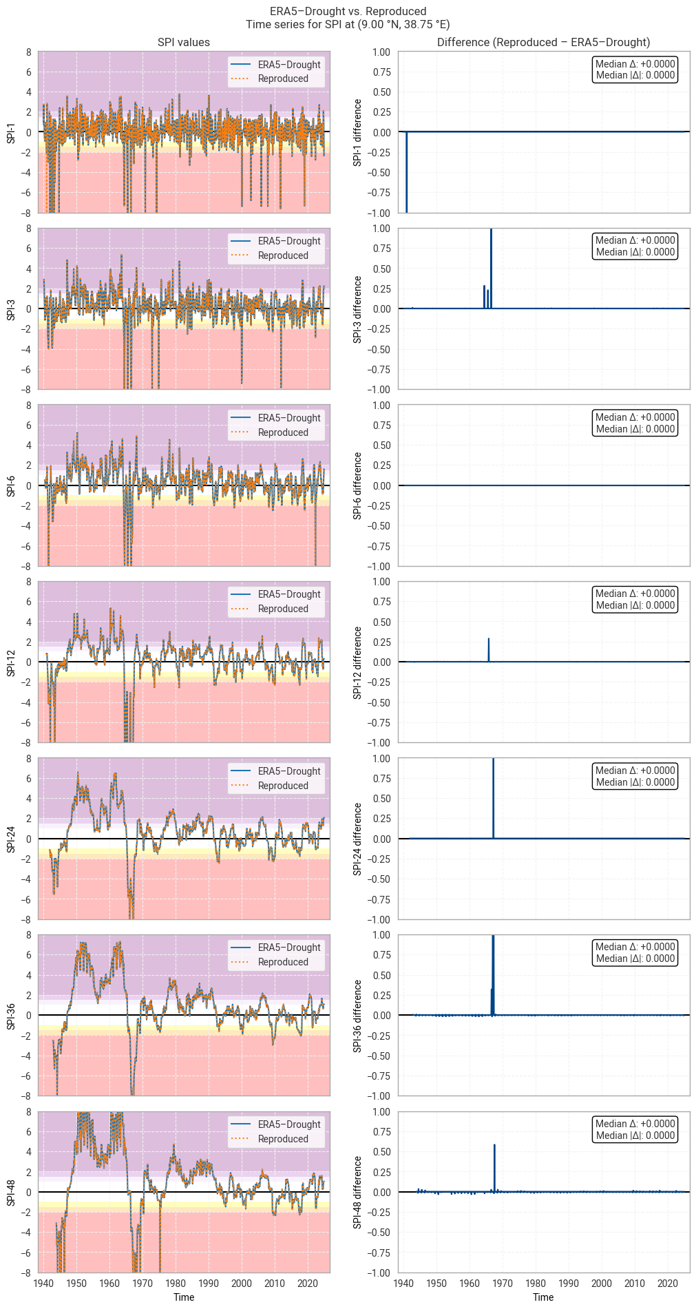
Fig. 6.1.2 SPI time series downloaded from ERA5–Drought and reproduced from ERA5 precipitation data (left) and the difference between the two (right), for the example site of Addis Ababa, Ethiopia. Colours in the left-hand column correspond to SPI categories (e.g. “extremely dry”) in [Keune+25].

Confusion matrix

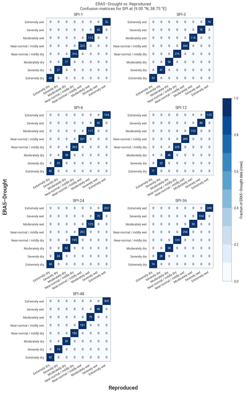
Fig. 6.1.3 Confusion matrices for SPI categories from ERA5–Drought vs. reproduced from ERA5, for the example site of Addis Ababa, Ethiopia, in 1940–2024.

3.7 SPI comparison: Regional snapshot

Next, we investigate spatial patterns in SPI and the difference therein across a wider region around the example site. This region is defined in 2. General setup. In this example, we look at part of the Horn of Africa using a box of 12° in all directions around Addis Ababa, Ethiopia. To reduce computing requirements, the comparison is performed for one year only, here 2024, again defined in 2. General setup.

As in the time series comparison, we subselect the desired data from ERA5 and calculate the corresponding SPI and download SPI from ERA5–Drought for the desired region and time span:

Show code cell source

Hide code cell source

# Select only desired site
data_era5_precipitation_region = data_era5_precipitation_preprocessed.sel(**example_region)

# Window in which to evaluate SPI
evaluation_window = {"time": slice(f"{year_snapshot}-01-01", f"{year_snapshot}-12-01")}  #  Slice (2024-01-01, 2024-12-01)

# Calculate SPI
spi_reproduced_region = calculate_spi_from_era5(data_era5_precipitation_region, reference_window=reference_window,
                                                evaluation_window=evaluation_window)

# Persist in memory to speed up analysis – this step may take a few minutes
spi_reproduced_region = spi_reproduced_region.persist()

# Display result
spi_reproduced_region

Show code cell output

Hide code cell output

<xarray.Dataset> Size: 6MB
Dimensions:  (lat: 97, lon: 97, time: 12)
Coordinates:
    number   int64 8B 0
  * lat      (lat) float64 776B 21.0 20.75 20.5 20.25 ... -2.25 -2.5 -2.75 -3.0
  * lon      (lon) float64 776B 26.75 27.0 27.25 27.5 ... 50.0 50.25 50.5 50.75
    month    (time) int64 96B dask.array<chunksize=(12,), meta=np.ndarray>
  * time     (time) datetime64[ns] 96B 2024-01-01T06:00:00 ... 2024-12-01T06:...
    expver   (time) <U4 192B dask.array<chunksize=(12,), meta=np.ndarray>
Data variables:
    SPI1     (lat, lon, time) float64 903kB dask.array<chunksize=(33, 97, 12), meta=np.ndarray>
    SPI3     (lat, lon, time) float64 903kB dask.array<chunksize=(33, 97, 12), meta=np.ndarray>
    SPI6     (lat, lon, time) float64 903kB dask.array<chunksize=(33, 97, 12), meta=np.ndarray>
    SPI12    (lat, lon, time) float64 903kB dask.array<chunksize=(33, 97, 12), meta=np.ndarray>
    SPI24    (lat, lon, time) float64 903kB dask.array<chunksize=(33, 97, 12), meta=np.ndarray>
    SPI36    (lat, lon, time) float64 903kB dask.array<chunksize=(33, 97, 12), meta=np.ndarray>
    SPI48    (lat, lon, time) float64 903kB dask.array<chunksize=(33, 97, 12), meta=np.ndarray>

xarray.Dataset

• Dimensions:
  • lat: 97
  • lon: 97
  • time: 12
• Coordinates: (6)
  • number
    ()
    int64
    0

    array(0)

  • lat
    (lat)
    float64
    21.0 20.75 20.5 ... -2.5 -2.75 -3.0

    array([21.  , 20.75, 20.5 , 20.25, 20.  , 19.75, 19.5 , 19.25, 19.  , 18.75,
           18.5 , 18.25, 18.  , 17.75, 17.5 , 17.25, 17.  , 16.75, 16.5 , 16.25,
           16.  , 15.75, 15.5 , 15.25, 15.  , 14.75, 14.5 , 14.25, 14.  , 13.75,
           13.5 , 13.25, 13.  , 12.75, 12.5 , 12.25, 12.  , 11.75, 11.5 , 11.25,
           11.  , 10.75, 10.5 , 10.25, 10.  ,  9.75,  9.5 ,  9.25,  9.  ,  8.75,
            8.5 ,  8.25,  8.  ,  7.75,  7.5 ,  7.25,  7.  ,  6.75,  6.5 ,  6.25,
            6.  ,  5.75,  5.5 ,  5.25,  5.  ,  4.75,  4.5 ,  4.25,  4.  ,  3.75,
            3.5 ,  3.25,  3.  ,  2.75,  2.5 ,  2.25,  2.  ,  1.75,  1.5 ,  1.25,
            1.  ,  0.75,  0.5 ,  0.25,  0.  , -0.25, -0.5 , -0.75, -1.  , -1.25,
           -1.5 , -1.75, -2.  , -2.25, -2.5 , -2.75, -3.  ])

  • lon
    (lon)
    float64
    26.75 27.0 27.25 ... 50.5 50.75

    array([26.75, 27.  , 27.25, 27.5 , 27.75, 28.  , 28.25, 28.5 , 28.75, 29.  ,
           29.25, 29.5 , 29.75, 30.  , 30.25, 30.5 , 30.75, 31.  , 31.25, 31.5 ,
           31.75, 32.  , 32.25, 32.5 , 32.75, 33.  , 33.25, 33.5 , 33.75, 34.  ,
           34.25, 34.5 , 34.75, 35.  , 35.25, 35.5 , 35.75, 36.  , 36.25, 36.5 ,
           36.75, 37.  , 37.25, 37.5 , 37.75, 38.  , 38.25, 38.5 , 38.75, 39.  ,
           39.25, 39.5 , 39.75, 40.  , 40.25, 40.5 , 40.75, 41.  , 41.25, 41.5 ,
           41.75, 42.  , 42.25, 42.5 , 42.75, 43.  , 43.25, 43.5 , 43.75, 44.  ,
           44.25, 44.5 , 44.75, 45.  , 45.25, 45.5 , 45.75, 46.  , 46.25, 46.5 ,
           46.75, 47.  , 47.25, 47.5 , 47.75, 48.  , 48.25, 48.5 , 48.75, 49.  ,
           49.25, 49.5 , 49.75, 50.  , 50.25, 50.5 , 50.75])

  • month
    (time)
    int64
    dask.array<chunksize=(12,), meta=np.ndarray>

    Array Chunk Bytes 96 B 96 B Shape (12,) (12,) Dask graph 1 chunks in 1 graph layer Data type int64 numpy.ndarray

  • time
    (time)
    datetime64[ns]
    2024-01-01T06:00:00 ... 2024-12-...

    long_name :

    time

    standard_name :

    time

    array(['2024-01-01T06:00:00.000000000', '2024-02-01T06:00:00.000000000',
           '2024-03-01T06:00:00.000000000', '2024-04-01T06:00:00.000000000',
           '2024-05-01T06:00:00.000000000', '2024-06-01T06:00:00.000000000',
           '2024-07-01T06:00:00.000000000', '2024-08-01T06:00:00.000000000',
           '2024-09-01T06:00:00.000000000', '2024-10-01T06:00:00.000000000',
           '2024-11-01T06:00:00.000000000', '2024-12-01T06:00:00.000000000'],
          dtype='datetime64[ns]')

  • expver
    (time)
    <U4
    dask.array<chunksize=(12,), meta=np.ndarray>

    Array Chunk Bytes 192 B 192 B Shape (12,) (12,) Dask graph 1 chunks in 1 graph layer Data type

• Data variables: (7)
  • SPI1
    (lat, lon, time)
    float64
    dask.array<chunksize=(33, 97, 12), meta=np.ndarray>

    Array Chunk Bytes 882.09 kiB 582.00 kiB Shape (97, 97, 12) (64, 97, 12) Dask graph 2 chunks in 1 graph layer Data type float64 numpy.ndarray

  • SPI3
    (lat, lon, time)
    float64
    dask.array<chunksize=(33, 97, 12), meta=np.ndarray>

    Array Chunk Bytes 882.09 kiB 582.00 kiB Shape (97, 97, 12) (64, 97, 12) Dask graph 2 chunks in 1 graph layer Data type float64 numpy.ndarray

  • SPI6
    (lat, lon, time)
    float64
    dask.array<chunksize=(33, 97, 12), meta=np.ndarray>

    Array Chunk Bytes 882.09 kiB 582.00 kiB Shape (97, 97, 12) (64, 97, 12) Dask graph 2 chunks in 1 graph layer Data type float64 numpy.ndarray

  • SPI12
    (lat, lon, time)
    float64
    dask.array<chunksize=(33, 97, 12), meta=np.ndarray>

    Array Chunk Bytes 882.09 kiB 582.00 kiB Shape (97, 97, 12) (64, 97, 12) Dask graph 2 chunks in 1 graph layer Data type float64 numpy.ndarray

  • SPI24
    (lat, lon, time)
    float64
    dask.array<chunksize=(33, 97, 12), meta=np.ndarray>

    Array Chunk Bytes 882.09 kiB 582.00 kiB Shape (97, 97, 12) (64, 97, 12) Dask graph 2 chunks in 1 graph layer Data type float64 numpy.ndarray

  • SPI36
    (lat, lon, time)
    float64
    dask.array<chunksize=(33, 97, 12), meta=np.ndarray>

    Array Chunk Bytes 882.09 kiB 582.00 kiB Shape (97, 97, 12) (64, 97, 12) Dask graph 2 chunks in 1 graph layer Data type float64 numpy.ndarray

  • SPI48
    (lat, lon, time)
    float64
    dask.array<chunksize=(33, 97, 12), meta=np.ndarray>

    Array Chunk Bytes 882.09 kiB 582.00 kiB Shape (97, 97, 12) (64, 97, 12) Dask graph 2 chunks in 1 graph layer Data type float64 numpy.ndarray

• Indexes: (3)
  • lat
    PandasIndex

    PandasIndex(Index([ 21.0, 20.75,  20.5, 20.25,  20.0, 19.75,  19.5, 19.25,  19.0, 18.75,
            18.5, 18.25,  18.0, 17.75,  17.5, 17.25,  17.0, 16.75,  16.5, 16.25,
            16.0, 15.75,  15.5, 15.25,  15.0, 14.75,  14.5, 14.25,  14.0, 13.75,
            13.5, 13.25,  13.0, 12.75,  12.5, 12.25,  12.0, 11.75,  11.5, 11.25,
            11.0, 10.75,  10.5, 10.25,  10.0,  9.75,   9.5,  9.25,   9.0,  8.75,
             8.5,  8.25,   8.0,  7.75,   7.5,  7.25,   7.0,  6.75,   6.5,  6.25,
             6.0,  5.75,   5.5,  5.25,   5.0,  4.75,   4.5,  4.25,   4.0,  3.75,
             3.5,  3.25,   3.0,  2.75,   2.5,  2.25,   2.0,  1.75,   1.5,  1.25,
             1.0,  0.75,   0.5,  0.25,   0.0, -0.25,  -0.5, -0.75,  -1.0, -1.25,
            -1.5, -1.75,  -2.0, -2.25,  -2.5, -2.75,  -3.0],
          dtype='float64', name='lat'))

  • lon
    PandasIndex

    PandasIndex(Index([26.75,  27.0, 27.25,  27.5, 27.75,  28.0, 28.25,  28.5, 28.75,  29.0,
           29.25,  29.5, 29.75,  30.0, 30.25,  30.5, 30.75,  31.0, 31.25,  31.5,
           31.75,  32.0, 32.25,  32.5, 32.75,  33.0, 33.25,  33.5, 33.75,  34.0,
           34.25,  34.5, 34.75,  35.0, 35.25,  35.5, 35.75,  36.0, 36.25,  36.5,
           36.75,  37.0, 37.25,  37.5, 37.75,  38.0, 38.25,  38.5, 38.75,  39.0,
           39.25,  39.5, 39.75,  40.0, 40.25,  40.5, 40.75,  41.0, 41.25,  41.5,
           41.75,  42.0, 42.25,  42.5, 42.75,  43.0, 43.25,  43.5, 43.75,  44.0,
           44.25,  44.5, 44.75,  45.0, 45.25,  45.5, 45.75,  46.0, 46.25,  46.5,
           46.75,  47.0, 47.25,  47.5, 47.75,  48.0, 48.25,  48.5, 48.75,  49.0,
           49.25,  49.5, 49.75,  50.0, 50.25,  50.5, 50.75],
          dtype='float64', name='lon'))

  • time
    PandasIndex

    PandasIndex(DatetimeIndex(['2024-01-01 06:00:00', '2024-02-01 06:00:00',
                   '2024-03-01 06:00:00', '2024-04-01 06:00:00',
                   '2024-05-01 06:00:00', '2024-06-01 06:00:00',
                   '2024-07-01 06:00:00', '2024-08-01 06:00:00',
                   '2024-09-01 06:00:00', '2024-10-01 06:00:00',
                   '2024-11-01 06:00:00', '2024-12-01 06:00:00'],
                  dtype='datetime64[ns]', name='time', freq=None))

• Attributes: (0)

Show code cell source

Hide code cell source

# Main request, based on template and example region
request_era5drought_spi = {
    "variable": ["standardised_precipitation_index"],
} | request_era5drought_index | request_region

# Select only desired year
request_era5drought_spi = request_era5drought_spi | {"year": [f"{year_snapshot}"],}

# Download data and load into xarray
spi_era5drought_region = ekd.from_source("cds", ID_ERA5_DROUGHT, request_era5drought_spi)
spi_era5drought_region = spi_era5drought_region.to_xarray(compat="equals", join="outer")
spi_era5drought_region = spi_era5drought_region.chunk({"time": -1})  # Full time series in one chunk

# Persist in memory to speed up analysis – this step may take a few minutes
spi_era5drought_region = spi_era5drought_region.persist()

# Display result
spi_era5drought_region

Show code cell output

Hide code cell output

<xarray.Dataset> Size: 6MB
Dimensions:  (time: 12, lat: 97, lon: 97)
Coordinates:
  * time     (time) datetime64[ns] 96B 2024-01-01T06:00:00 ... 2024-12-01T06:...
  * lat      (lat) float64 776B 21.0 20.75 20.5 20.25 ... -2.25 -2.5 -2.75 -3.0
  * lon      (lon) float64 776B 26.75 27.0 27.25 27.5 ... 50.0 50.25 50.5 50.75
Data variables:
    SPI12    (time, lat, lon) float64 903kB dask.array<chunksize=(12, 97, 97), meta=np.ndarray>
    SPI1     (time, lat, lon) float64 903kB dask.array<chunksize=(12, 97, 97), meta=np.ndarray>
    SPI24    (time, lat, lon) float64 903kB dask.array<chunksize=(12, 97, 97), meta=np.ndarray>
    SPI36    (time, lat, lon) float64 903kB dask.array<chunksize=(12, 97, 97), meta=np.ndarray>
    SPI3     (time, lat, lon) float64 903kB dask.array<chunksize=(12, 97, 97), meta=np.ndarray>
    SPI48    (time, lat, lon) float64 903kB dask.array<chunksize=(12, 97, 97), meta=np.ndarray>
    SPI6     (time, lat, lon) float64 903kB dask.array<chunksize=(12, 97, 97), meta=np.ndarray>
Attributes: (12/17)
    title:                   SPI12
    description:             Drought Index: Standardized Drought Index calcul...
    Conventions:             CF-1.8
    history:                 Created 30/10/2024 07:50:12 using DRYFALL.
    institution:             European Centre for Medium-Range Weather Forecasts
    source:                  DRYFALL v1.0
    ...                      ...
    climate_start_date:      1991-01-01
    climate_end_date:        2020-12-31
    frequency:               Monthly
    contact_person:          support@ecmwf.int
    ref_publication:         Keune, J., Di Giuseppe, F., Barnard, C., Damasio...
    cds_data_catalogue_url:  https://cds.climate.copernicus.eu/datasets/deriv...

xarray.Dataset

• Dimensions:
  • time: 12
  • lat: 97
  • lon: 97
• Coordinates: (3)
  • time
    (time)
    datetime64[ns]
    2024-01-01T06:00:00 ... 2024-12-...

    standard_name :

    time

    array(['2024-01-01T06:00:00.000000000', '2024-02-01T06:00:00.000000000',
           '2024-03-01T06:00:00.000000000', '2024-04-01T06:00:00.000000000',
           '2024-05-01T06:00:00.000000000', '2024-06-01T06:00:00.000000000',
           '2024-07-01T06:00:00.000000000', '2024-08-01T06:00:00.000000000',
           '2024-09-01T06:00:00.000000000', '2024-10-01T06:00:00.000000000',
           '2024-11-01T06:00:00.000000000', '2024-12-01T06:00:00.000000000'],
          dtype='datetime64[ns]')

  • lat
    (lat)
    float64
    21.0 20.75 20.5 ... -2.5 -2.75 -3.0

    units :

    degrees_north

    long_name :

    degrees_north

    array([21.  , 20.75, 20.5 , 20.25, 20.  , 19.75, 19.5 , 19.25, 19.  , 18.75,
           18.5 , 18.25, 18.  , 17.75, 17.5 , 17.25, 17.  , 16.75, 16.5 , 16.25,
           16.  , 15.75, 15.5 , 15.25, 15.  , 14.75, 14.5 , 14.25, 14.  , 13.75,
           13.5 , 13.25, 13.  , 12.75, 12.5 , 12.25, 12.  , 11.75, 11.5 , 11.25,
           11.  , 10.75, 10.5 , 10.25, 10.  ,  9.75,  9.5 ,  9.25,  9.  ,  8.75,
            8.5 ,  8.25,  8.  ,  7.75,  7.5 ,  7.25,  7.  ,  6.75,  6.5 ,  6.25,
            6.  ,  5.75,  5.5 ,  5.25,  5.  ,  4.75,  4.5 ,  4.25,  4.  ,  3.75,
            3.5 ,  3.25,  3.  ,  2.75,  2.5 ,  2.25,  2.  ,  1.75,  1.5 ,  1.25,
            1.  ,  0.75,  0.5 ,  0.25,  0.  , -0.25, -0.5 , -0.75, -1.  , -1.25,
           -1.5 , -1.75, -2.  , -2.25, -2.5 , -2.75, -3.  ])

  • lon
    (lon)
    float64
    26.75 27.0 27.25 ... 50.5 50.75

    units :

    degrees_east

    long_name :

    degrees_east

    array([26.75, 27.  , 27.25, 27.5 , 27.75, 28.  , 28.25, 28.5 , 28.75, 29.  ,
           29.25, 29.5 , 29.75, 30.  , 30.25, 30.5 , 30.75, 31.  , 31.25, 31.5 ,
           31.75, 32.  , 32.25, 32.5 , 32.75, 33.  , 33.25, 33.5 , 33.75, 34.  ,
           34.25, 34.5 , 34.75, 35.  , 35.25, 35.5 , 35.75, 36.  , 36.25, 36.5 ,
           36.75, 37.  , 37.25, 37.5 , 37.75, 38.  , 38.25, 38.5 , 38.75, 39.  ,
           39.25, 39.5 , 39.75, 40.  , 40.25, 40.5 , 40.75, 41.  , 41.25, 41.5 ,
           41.75, 42.  , 42.25, 42.5 , 42.75, 43.  , 43.25, 43.5 , 43.75, 44.  ,
           44.25, 44.5 , 44.75, 45.  , 45.25, 45.5 , 45.75, 46.  , 46.25, 46.5 ,
           46.75, 47.  , 47.25, 47.5 , 47.75, 48.  , 48.25, 48.5 , 48.75, 49.  ,
           49.25, 49.5 , 49.75, 50.  , 50.25, 50.5 , 50.75])

• Data variables: (7)
  • SPI12
    (time, lat, lon)
    float64
    dask.array<chunksize=(12, 97, 97), meta=np.ndarray>

    long_name :

    Standardized Drought Index (SPI12)

    Array Chunk Bytes 882.09 kiB 882.09 kiB Shape (12, 97, 97) (12, 97, 97) Dask graph 1 chunks in 1 graph layer Data type float64 numpy.ndarray

  • SPI1
    (time, lat, lon)
    float64
    dask.array<chunksize=(12, 97, 97), meta=np.ndarray>

    long_name :

    Standardized Drought Index (SPI1)

    Array Chunk Bytes 882.09 kiB 882.09 kiB Shape (12, 97, 97) (12, 97, 97) Dask graph 1 chunks in 1 graph layer Data type float64 numpy.ndarray

  • SPI24
    (time, lat, lon)
    float64
    dask.array<chunksize=(12, 97, 97), meta=np.ndarray>

    long_name :

    Standardized Drought Index (SPI24)

    Array Chunk Bytes 882.09 kiB 882.09 kiB Shape (12, 97, 97) (12, 97, 97) Dask graph 1 chunks in 1 graph layer Data type float64 numpy.ndarray

  • SPI36
    (time, lat, lon)
    float64
    dask.array<chunksize=(12, 97, 97), meta=np.ndarray>

    long_name :

    Standardized Drought Index (SPI36)

    Array Chunk Bytes 882.09 kiB 882.09 kiB Shape (12, 97, 97) (12, 97, 97) Dask graph 1 chunks in 1 graph layer Data type float64 numpy.ndarray

  • SPI3
    (time, lat, lon)
    float64
    dask.array<chunksize=(12, 97, 97), meta=np.ndarray>

    long_name :

    Standardized Drought Index (SPI3)

    Array Chunk Bytes 882.09 kiB 882.09 kiB Shape (12, 97, 97) (12, 97, 97) Dask graph 1 chunks in 1 graph layer Data type float64 numpy.ndarray

  • SPI48
    (time, lat, lon)
    float64
    dask.array<chunksize=(12, 97, 97), meta=np.ndarray>

    long_name :

    Standardized Drought Index (SPI48)

    Array Chunk Bytes 882.09 kiB 882.09 kiB Shape (12, 97, 97) (12, 97, 97) Dask graph 1 chunks in 1 graph layer Data type float64 numpy.ndarray

  • SPI6
    (time, lat, lon)
    float64
    dask.array<chunksize=(12, 97, 97), meta=np.ndarray>

    long_name :

    Standardized Drought Index (SPI6)

    Array Chunk Bytes 882.09 kiB 882.09 kiB Shape (12, 97, 97) (12, 97, 97) Dask graph 1 chunks in 1 graph layer Data type float64 numpy.ndarray

• Indexes: (3)
  • time
    PandasIndex

    PandasIndex(DatetimeIndex(['2024-01-01 06:00:00', '2024-02-01 06:00:00',
                   '2024-03-01 06:00:00', '2024-04-01 06:00:00',
                   '2024-05-01 06:00:00', '2024-06-01 06:00:00',
                   '2024-07-01 06:00:00', '2024-08-01 06:00:00',
                   '2024-09-01 06:00:00', '2024-10-01 06:00:00',
                   '2024-11-01 06:00:00', '2024-12-01 06:00:00'],
                  dtype='datetime64[ns]', name='time', freq=None))

  • lat
    PandasIndex

    PandasIndex(Index([ 21.0, 20.75,  20.5, 20.25,  20.0, 19.75,  19.5, 19.25,  19.0, 18.75,
            18.5, 18.25,  18.0, 17.75,  17.5, 17.25,  17.0, 16.75,  16.5, 16.25,
            16.0, 15.75,  15.5, 15.25,  15.0, 14.75,  14.5, 14.25,  14.0, 13.75,
            13.5, 13.25,  13.0, 12.75,  12.5, 12.25,  12.0, 11.75,  11.5, 11.25,
            11.0, 10.75,  10.5, 10.25,  10.0,  9.75,   9.5,  9.25,   9.0,  8.75,
             8.5,  8.25,   8.0,  7.75,   7.5,  7.25,   7.0,  6.75,   6.5,  6.25,
             6.0,  5.75,   5.5,  5.25,   5.0,  4.75,   4.5,  4.25,   4.0,  3.75,
             3.5,  3.25,   3.0,  2.75,   2.5,  2.25,   2.0,  1.75,   1.5,  1.25,
             1.0,  0.75,   0.5,  0.25,   0.0, -0.25,  -0.5, -0.75,  -1.0, -1.25,
            -1.5, -1.75,  -2.0, -2.25,  -2.5, -2.75,  -3.0],
          dtype='float64', name='lat'))

  • lon
    PandasIndex

    PandasIndex(Index([26.75,  27.0, 27.25,  27.5, 27.75,  28.0, 28.25,  28.5, 28.75,  29.0,
           29.25,  29.5, 29.75,  30.0, 30.25,  30.5, 30.75,  31.0, 31.25,  31.5,
           31.75,  32.0, 32.25,  32.5, 32.75,  33.0, 33.25,  33.5, 33.75,  34.0,
           34.25,  34.5, 34.75,  35.0, 35.25,  35.5, 35.75,  36.0, 36.25,  36.5,
           36.75,  37.0, 37.25,  37.5, 37.75,  38.0, 38.25,  38.5, 38.75,  39.0,
           39.25,  39.5, 39.75,  40.0, 40.25,  40.5, 40.75,  41.0, 41.25,  41.5,
           41.75,  42.0, 42.25,  42.5, 42.75,  43.0, 43.25,  43.5, 43.75,  44.0,
           44.25,  44.5, 44.75,  45.0, 45.25,  45.5, 45.75,  46.0, 46.25,  46.5,
           46.75,  47.0, 47.25,  47.5, 47.75,  48.0, 48.25,  48.5, 48.75,  49.0,
           49.25,  49.5, 49.75,  50.0, 50.25,  50.5, 50.75],
          dtype='float64', name='lon'))

• Attributes: (17)

  title :

  SPI12

  description :

  Drought Index: Standardized Drought Index calculated according to the WMO guidelines (see https://library.wmo.int/doc_num.php?explnum_id=7768).

  Conventions :

  CF-1.8

  history :

  Created 30/10/2024 07:50:12 using DRYFALL.

  institution :

  European Centre for Medium-Range Weather Forecasts

  source :

  DRYFALL v1.0

  license :

  Creative Commons Attribution v4

  citation_statement :

  Drought indicators derived from ERA5 reanalysis

  data_srs :

  EPSG:4326

  extent :

  -180,-90,180,90

  resolution :

  0.25x0.25

  climate_start_date :

  1991-01-01

  climate_end_date :

  2020-12-31

  frequency :

  Monthly

  contact_person :

  support@ecmwf.int

  ref_publication :

  Keune, J., Di Giuseppe, F., Barnard, C., Damasio da Costa, E., and Wetterhall, F. (2025): ERA5–Drought: Global drought indices based on ECMWF reanalysis, Scientific Data 12, 616. https://doi.org/10.1038/s41597-025-04896-y

  cds_data_catalogue_url :

  https://cds.climate.copernicus.eu/datasets/derived-drought-historical-monthly

As before, we examine the per-point difference in SPI between ERA5–Drought and the reproduction for each calendar month and each accumulation period:

Show code cell source

Hide code cell source

# Calculate SPI median differences
spi_difference_region = comparison_monthly_statistics(spi_era5drought_region, spi_reproduced_region)

# Display with style
display_monthly_statistics(spi_difference_region)

Reproduced – ERA5–Drought

	SPI-1			SPI-3			SPI-6			SPI-12			SPI-24			SPI-36			SPI-48
	MΔ	M|Δ|	|Δ| ≥ 0.10	MΔ	M|Δ|	|Δ| ≥ 0.10	MΔ	M|Δ|	|Δ| ≥ 0.10	MΔ	M|Δ|	|Δ| ≥ 0.10	MΔ	M|Δ|	|Δ| ≥ 0.10	MΔ	M|Δ|	|Δ| ≥ 0.10	MΔ	M|Δ|	|Δ| ≥ 0.10
January	0.0000	0.0000	15.5702	0.0000	0.0000	8.7576	0.0000	0.0000	6.8658	0.0000	0.0000	1.2754	0.0000	0.0000	16.4842	0.0000	0.0000	0.0106	0.0000	0.0000	0.0000
February	0.0000	0.0000	20.0128	0.0000	0.0000	8.5556	0.0000	0.0000	6.9402	0.0000	0.0000	1.5730	0.0000	0.0000	16.5374	0.0000	0.0000	0.0425	0.0000	0.0000	0.0319
March	0.0000	0.0000	18.1422	0.0000	0.0000	11.7653	0.0000	0.0000	7.3228	0.0000	0.0000	1.2754	0.0000	0.0000	16.5374	0.0000	0.0000	0.0213	0.0000	0.0000	0.0000
April	0.0000	0.0000	10.3093	0.0000	0.0000	11.5315	0.0000	0.0000	11.4146	0.0000	0.0000	1.4454	0.0000	0.0000	16.5586	0.0000	0.0000	0.0425	0.0000	0.0000	0.0000
May	0.0000	0.0000	10.8194	0.0000	0.0000	6.7701	0.0000	0.0000	5.6116	0.0000	0.0000	1.4135	0.0000	0.0000	16.5055	0.0000	0.0000	0.0425	0.0000	0.0000	0.0213
June	0.0000	0.0000	8.2155	0.0000	0.0000	6.3237	0.0000	0.0000	5.2078	0.0000	0.0000	1.4879	0.0000	0.0000	16.4948	0.0000	0.0000	0.0744	0.0000	0.0000	0.0531
July	0.0000	0.0000	12.1586	0.0000	0.0000	9.2571	0.0000	0.0000	5.6648	0.0000	0.0000	0.9884	0.0000	0.0000	16.4523	0.0000	0.0000	0.0531	0.0000	0.0000	0.0744
August	0.0000	0.0000	14.2842	0.0000	0.0000	8.0242	0.0000	0.0000	2.7527	0.0000	0.0000	1.3285	0.0000	0.0000	16.4842	0.0000	0.0000	0.0213	0.0000	0.0000	0.0744
September	0.0000	0.0000	8.7895	0.0000	0.0000	7.7798	0.0000	0.0000	3.3797	0.0000	0.0000	1.2329	0.0000	0.0000	16.4948	0.0000	0.0000	0.0213	0.0000	0.0000	0.0638
October	0.0000	0.0000	7.4397	0.0000	0.0000	6.7063	0.0000	0.0000	4.2406	0.0000	0.0000	1.5836	0.0000	0.0000	16.4630	0.0000	0.0000	0.0319	0.0000	0.0000	0.0213
November	0.0000	0.0000	8.2581	0.0000	0.0000	9.0764	0.0000	0.0000	4.5913	0.0000	0.0000	1.2435	0.0000	0.0000	16.4523	0.0000	0.0000	0.0425	0.0000	0.0000	0.0213
December	0.0000	0.0000	10.1711	0.0000	0.0000	7.6204	0.0000	0.0000	4.4851	0.0000	0.0000	1.3073	0.0000	0.0000	16.4948	0.0000	0.0000	0.0319	0.0000	0.0000	0.0425

As before, the differences between ERA5–Drought and reproduced SPI are small to zero in most cases. Notably, differences of more than 0.10 appear in a larger number of match-ups than before, more commonly for short accumulation periods than for long ones. This is likely because the time series for longer accumulation periods are smoother, which makes it easier for the fitting procedure to converge on the same optimal parameters. There is no clear cause for certain months showing more difference than others, such as local seasonal trends [Gebrechorkos+19], although the region may be too large and diverse to draw such correlations.

The distribution across the example region (Figure 6.1.4) shows that for SPI-3 and longer, discrepancies are concentrated in deserts (Sahara, Arabian peninsula) where zero-precipitation months are common and hence it is harder to appropriately fit SPI. In fact, many of these areas are flagged for low data quality or even not fitted at all in ERA5–Drought, as discussed in the next subsection. For SPI-1, differences between the two datasets appear more randomly spread out. Note that the grey area in the top left of the reproduced SPI-1 panel (Sudan) corresponds to NaN values, i.e. areas where the fitting procedure could not converge at all. Lastly, the large differences in SPI-24 are seemingly due to an issue with ERA5–Drought’s land-sea mask; SPI-24 is –9999 on all water pixels in ERA5–Drought, which is clearly a filler value and not real data. We have not applied a land-sea mask to the reproduction, causing these large differences in SPI-24 only.

The generally good agreement in SPI translates into good agreement in classification (Figure 6.1.5), although some pixels do get classified differently in ERA5–Drought vs. the reproduced dataset. Mismatches occur mostly between adjacent categories (e.g. “moderately wet” and “severely wet”), although there are outliers in shorter accumulation periods; some of these likely correspond to pixels where quality flags would normally be applied [Keune+25].

Show code cell source

Hide code cell source

# Plot geospatial comparison: SPI in one region
plot_geospatial_comparison(spi_era5drought_region, spi_reproduced_region, var="SPI", time=f"{year_snapshot}-12-01",
                           domain=domain_region,
                           glue_label="indicator_derived-drought-historical-monthly_consistency_q01_fig-spi-geospatial")

Show code cell source

Hide code cell source

# Plot confusion matrix comparison
# e.g. are all "extremely dry" data in ERA5–Drought also "extremely dry" in the reproduction?
plot_confusion_matrices_spi(spi_era5drought_region, spi_reproduced_region, title_suffix=f" in {label_region}",
                            glue_label="indicator_derived-drought-historical-monthly_consistency_q01_fig-spi-confusion-region")

Geospatial

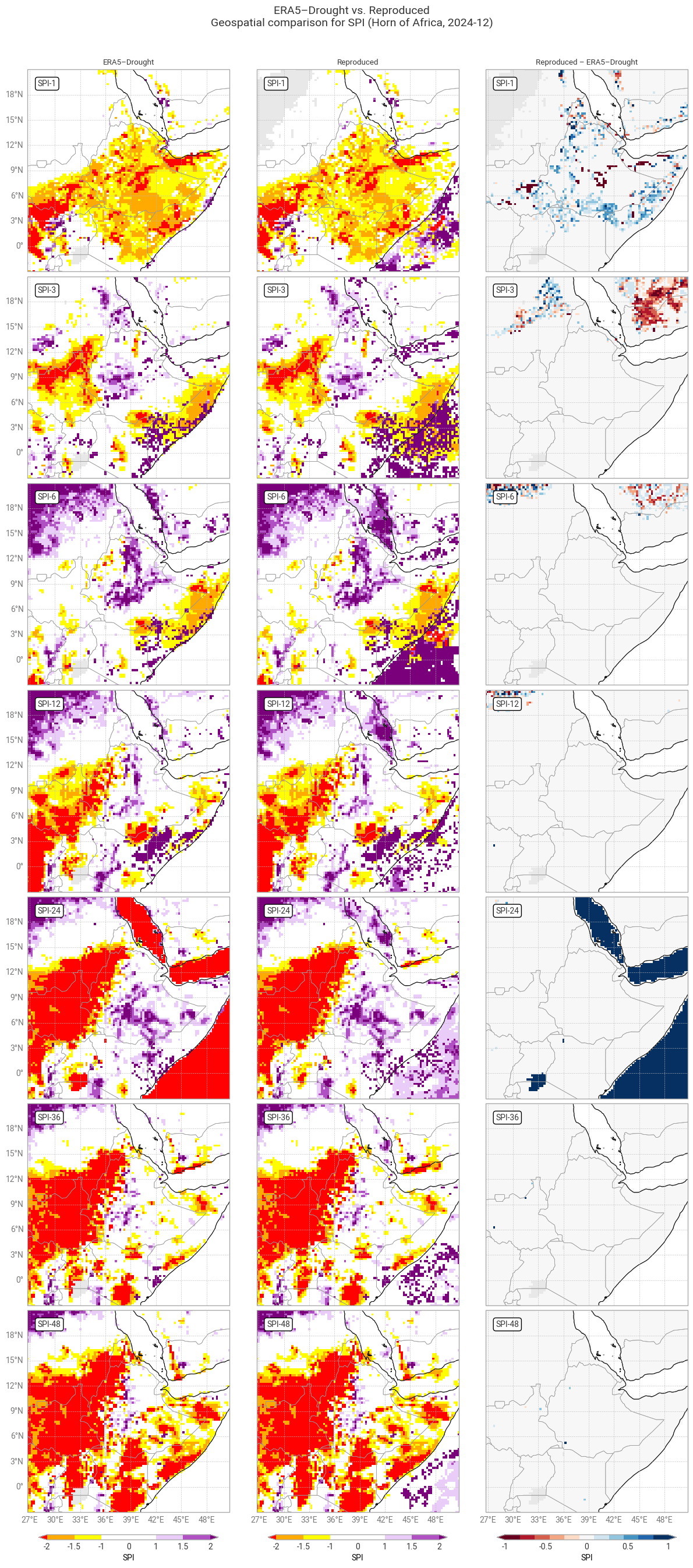
Fig. 6.1.4 SPI downloaded from ERA5–Drought (left) vs. reproduced from ERA5 precipitation data (middle) and the difference between the two (right), for the region around the example site of Addis Ababa, Ethiopia. Only one month (December 2024) is displayed. Colours correspond to SPI categories (e.g. “extremely dry”) in [Keune+25].

Confusion matrix

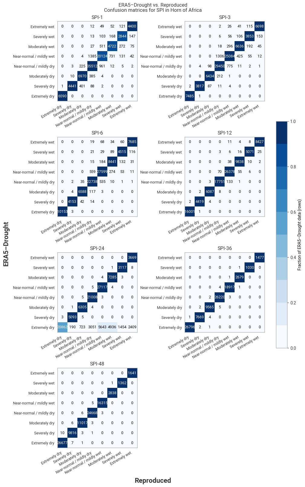
Fig. 6.1.5 Confusion matrices for SPI categories from ERA5–Drought vs. reproduced from ERA5, across the region around the example site of Addis Ababa, Ethiopia. Combines data for all months within one year (2024).

3.8 Quality flags: Probability of zero precipitation

One of the quality flags included in ERA5–Drought is the probability of zero precipitation p₀. This represents, for each calendar month and accumulation period, the fraction of months within the reference period (1991–2020) where precipitation was zero. While the ERA5–Drought implementation of SPI accounts for months with zero precipitation by shifting the CDF, as demonstrated above, those months do skew the fitted distribution and reduce the reliability of the index. In ERA5–Drought, the gamma distribution is not even fitted if at least 10 out of 30 months in the reference window have 0 precipitation, and the authors recommend that users filter out locations with a lower threshold, such as p₀ > 0.1 [Keune+25].

Unlike the zero-precipitation correction, this quality flag uses an unweighted probability, with n₀ the number of months with zero precipitation and n the total number of months in the reference window (30):

\[ p_0 = \frac{n_0}{n + 1} \]

In this subsection, we reproduce the p₀ quality flag and its derived masks, and compare their values to those provided in ERA5–Drought.

Show code cell source

Hide code cell source

# Accumulate total precipitation
data_era5_precipitation = accumulate(data_era5_precipitation_preprocessed, "tp")

# Select data in reference window
data_era5_precipitation_reference = data_era5_precipitation.sel(**reference_window)

# Calculate the probability of zero precipitation
p_zero_reproduced = probability_of_zero_precipitation(data_era5_precipitation_reference)

# Retain in memory
p_zero_reproduced = p_zero_reproduced.persist()

# Display result
p_zero_reproduced

Show code cell output

Hide code cell output

<xarray.Dataset> Size: 698MB
Dimensions:  (lat: 721, lon: 1440, month: 12)
Coordinates:
    number   int64 8B 0
  * lat      (lat) float64 6kB 90.0 89.75 89.5 89.25 ... -89.5 -89.75 -90.0
  * lon      (lon) float64 12kB -180.0 -179.8 -179.5 ... 179.2 179.5 179.8
  * month    (month) int64 96B 1 2 3 4 5 6 7 8 9 10 11 12
Data variables:
    tp1      (month, lat, lon) float64 100MB dask.array<chunksize=(1, 103, 360), meta=np.ndarray>
    tp3      (month, lat, lon) float64 100MB dask.array<chunksize=(1, 103, 360), meta=np.ndarray>
    tp6      (month, lat, lon) float64 100MB dask.array<chunksize=(1, 103, 360), meta=np.ndarray>
    tp12     (month, lat, lon) float64 100MB dask.array<chunksize=(1, 103, 360), meta=np.ndarray>
    tp24     (month, lat, lon) float64 100MB dask.array<chunksize=(1, 103, 360), meta=np.ndarray>
    tp36     (month, lat, lon) float64 100MB dask.array<chunksize=(1, 103, 360), meta=np.ndarray>
    tp48     (month, lat, lon) float64 100MB dask.array<chunksize=(1, 103, 360), meta=np.ndarray>

xarray.Dataset

• Dimensions:
  • lat: 721
  • lon: 1440
  • month: 12
• Coordinates: (4)
  • number
    ()
    int64
    0

    long_name :

    ensemble member numerical id

    units :

    1

    standard_name :

    realization

    array(0)

  • lat
    (lat)
    float64
    90.0 89.75 89.5 ... -89.75 -90.0

    units :

    degrees_north

    standard_name :

    latitude

    long_name :

    latitude

    stored_direction :

    decreasing

    array([ 90.  ,  89.75,  89.5 , ..., -89.5 , -89.75, -90.  ], shape=(721,))

  • lon
    (lon)
    float64
    -180.0 -179.8 ... 179.5 179.8

    array([-180.  , -179.75, -179.5 , ...,  179.25,  179.5 ,  179.75],
          shape=(1440,))

  • month
    (month)
    int64
    1 2 3 4 5 6 7 8 9 10 11 12

    long_name :

    time

    standard_name :

    time

    array([ 1,  2,  3,  4,  5,  6,  7,  8,  9, 10, 11, 12])

• Data variables: (7)
  • tp1
    (month, lat, lon)
    float64
    dask.array<chunksize=(1, 103, 360), meta=np.ndarray>

    Array Chunk Bytes 95.05 MiB 289.69 kiB Shape (12, 721, 1440) (1, 103, 360) Dask graph 336 chunks in 1 graph layer Data type float64 numpy.ndarray

  • tp3
    (month, lat, lon)
    float64
    dask.array<chunksize=(1, 103, 360), meta=np.ndarray>

    Array Chunk Bytes 95.05 MiB 289.69 kiB Shape (12, 721, 1440) (1, 103, 360) Dask graph 336 chunks in 1 graph layer Data type float64 numpy.ndarray

  • tp6
    (month, lat, lon)
    float64
    dask.array<chunksize=(1, 103, 360), meta=np.ndarray>

    Array Chunk Bytes 95.05 MiB 289.69 kiB Shape (12, 721, 1440) (1, 103, 360) Dask graph 336 chunks in 1 graph layer Data type float64 numpy.ndarray

  • tp12
    (month, lat, lon)
    float64
    dask.array<chunksize=(1, 103, 360), meta=np.ndarray>

    Array Chunk Bytes 95.05 MiB 289.69 kiB Shape (12, 721, 1440) (1, 103, 360) Dask graph 336 chunks in 1 graph layer Data type float64 numpy.ndarray

  • tp24
    (month, lat, lon)
    float64
    dask.array<chunksize=(1, 103, 360), meta=np.ndarray>

    Array Chunk Bytes 95.05 MiB 289.69 kiB Shape (12, 721, 1440) (1, 103, 360) Dask graph 336 chunks in 1 graph layer Data type float64 numpy.ndarray

  • tp36
    (month, lat, lon)
    float64
    dask.array<chunksize=(1, 103, 360), meta=np.ndarray>

    Array Chunk Bytes 95.05 MiB 289.69 kiB Shape (12, 721, 1440) (1, 103, 360) Dask graph 336 chunks in 1 graph layer Data type float64 numpy.ndarray

  • tp48
    (month, lat, lon)
    float64
    dask.array<chunksize=(1, 103, 360), meta=np.ndarray>

    Array Chunk Bytes 95.05 MiB 289.69 kiB Shape (12, 721, 1440) (1, 103, 360) Dask graph 336 chunks in 1 graph layer Data type float64 numpy.ndarray

• Indexes: (3)
  • lat
    PandasIndex

    PandasIndex(Index([  90.0,  89.75,   89.5,  89.25,   89.0,  88.75,   88.5,  88.25,   88.0,
            87.75,
           ...
           -87.75,  -88.0, -88.25,  -88.5, -88.75,  -89.0, -89.25,  -89.5, -89.75,
            -90.0],
          dtype='float64', name='lat', length=721))

  • lon
    PandasIndex

    PandasIndex(Index([ -180.0, -179.75,  -179.5, -179.25,  -179.0, -178.75,  -178.5, -178.25,
            -178.0, -177.75,
           ...
             177.5,  177.75,   178.0,  178.25,   178.5,  178.75,   179.0,  179.25,
             179.5,  179.75],
          dtype='float64', name='lon', length=1440))

  • month
    PandasIndex

    PandasIndex(Index([1, 2, 3, 4, 5, 6, 7, 8, 9, 10, 11, 12], dtype='int64', name='month'))

• Attributes: (0)

The CDS provides ERA5–Drought’s p₀ flag for each accumulation period, but does not distinguish between them in the variable name. This means that p₀ must be downloaded separately for each accumulation period, renamed, and merged together, rather than downloading it for all simultaneously:

Show code cell source

Hide code cell source

# Setup: Request for each accumulation period
request_p_zero = {
    "variable": ["probability_of_zero_precipitation_spi"],
} | request_era5drought_flag

requests_per_accumulation_period = {period: {"accumulation_period": [str(period)],}
                                    for period in ACCUMULATION_PERIODS}

subrequests_era5drought_p_zero = {period: (req | request_p_zero)
                                  for period, req in requests_per_accumulation_period.items()}

# Download data in individual requests
p_zero_era5drought = {period: ekd.from_source("cds", ID_ERA5_DROUGHT, subreq)  # Download as field lists
                      for period, subreq in subrequests_era5drought_p_zero.items()}

# Pre-process: Convert to xarray, handle variable names, month dimension
p_zero_era5drought = preprocess_era5drought_qualityflag(p_zero_era5drought, "tp")

# Display in notebook
p_zero_era5drought

Show code cell output

Hide code cell output

<xarray.Dataset> Size: 698MB
Dimensions:  (month: 12, lat: 721, lon: 1440)
Coordinates:
    time     (month) datetime64[ns] 96B 2020-01-01 2020-02-01 ... 2020-12-01
  * lon      (lon) float64 12kB -180.0 -179.8 -179.5 ... 179.2 179.5 179.8
  * lat      (lat) float64 6kB 90.0 89.75 89.5 89.25 ... -89.5 -89.75 -90.0
  * month    (month) int64 96B 1 2 3 4 5 6 7 8 9 10 11 12
Data variables:
    tp1      (month, lat, lon) float64 100MB dask.array<chunksize=(1, 721, 1440), meta=np.ndarray>
    tp3      (month, lat, lon) float64 100MB dask.array<chunksize=(1, 721, 1440), meta=np.ndarray>
    tp6      (month, lat, lon) float64 100MB dask.array<chunksize=(1, 721, 1440), meta=np.ndarray>
    tp12     (month, lat, lon) float64 100MB dask.array<chunksize=(1, 721, 1440), meta=np.ndarray>
    tp24     (month, lat, lon) float64 100MB dask.array<chunksize=(1, 721, 1440), meta=np.ndarray>
    tp36     (month, lat, lon) float64 100MB dask.array<chunksize=(1, 721, 1440), meta=np.ndarray>
    tp48     (month, lat, lon) float64 100MB dask.array<chunksize=(1, 721, 1440), meta=np.ndarray>
Attributes: (12/19)
    CDI:                     Climate Data Interface version 1.9.10 (https://m...
    Conventions:             CF-1.8
    source:                  DRYFALL v1.0
    institution:             European Centre for Medium-Range Weather Forecasts
    title:                   Quality criteria for the derived standardized dr...
    description:             Monthly quality criteria that define the reliabi...
    ...                      ...
    resolution:              0.25x0.25
    climate_start_date:      1991-01-01
    climate_end_date:        2020-12-31
    frequency:               Monthly
    contact_person:          support@ecmwf.int
    CDO:                     Climate Data Operators version 1.9.10 (https://m...

xarray.Dataset

• Dimensions:
  • month: 12
  • lat: 721
  • lon: 1440
• Coordinates: (4)
  • time
    (month)
    datetime64[ns]
    2020-01-01 ... 2020-12-01

    standard_name :

    time

    axis :

    T

    array(['2020-01-01T00:00:00.000000000', '2020-02-01T00:00:00.000000000',
           '2020-03-01T00:00:00.000000000', '2020-04-01T00:00:00.000000000',
           '2020-05-01T00:00:00.000000000', '2020-06-01T00:00:00.000000000',
           '2020-07-01T00:00:00.000000000', '2020-08-01T00:00:00.000000000',
           '2020-09-01T00:00:00.000000000', '2020-10-01T00:00:00.000000000',
           '2020-11-01T00:00:00.000000000', '2020-12-01T00:00:00.000000000'],
          dtype='datetime64[ns]')

  • lon
    (lon)
    float64
    -180.0 -179.8 ... 179.5 179.8

    standard_name :

    longitude

    long_name :

    longitude

    units :

    degrees_east

    axis :

    X

    array([-180.  , -179.75, -179.5 , ...,  179.25,  179.5 ,  179.75],
          shape=(1440,))

  • lat
    (lat)
    float64
    90.0 89.75 89.5 ... -89.75 -90.0

    standard_name :

    latitude

    long_name :

    latitude

    units :

    degrees_north

    axis :

    Y

    array([ 90.  ,  89.75,  89.5 , ..., -89.5 , -89.75, -90.  ], shape=(721,))

  • month
    (month)
    int64
    1 2 3 4 5 6 7 8 9 10 11 12

    standard_name :

    time

    axis :

    T

    array([ 1,  2,  3,  4,  5,  6,  7,  8,  9, 10, 11, 12])

• Data variables: (7)
  • tp1
    (month, lat, lon)
    float64
    dask.array<chunksize=(1, 721, 1440), meta=np.ndarray>

    long_name :

    Number of months with zero precipitation during the reference period expressed as the fraction of the total number of months

    units :

    1

    Array Chunk Bytes 95.05 MiB 7.92 MiB Shape (12, 721, 1440) (1, 721, 1440) Dask graph 12 chunks in 25 graph layers Data type float64 numpy.ndarray

  • tp3
    (month, lat, lon)
    float64
    dask.array<chunksize=(1, 721, 1440), meta=np.ndarray>

    long_name :

    Number of months with zero precipitation during the reference period expressed as the fraction of the total number of months

    units :

    1

    Array Chunk Bytes 95.05 MiB 7.92 MiB Shape (12, 721, 1440) (1, 721, 1440) Dask graph 12 chunks in 25 graph layers Data type float64 numpy.ndarray

  • tp6
    (month, lat, lon)
    float64
    dask.array<chunksize=(1, 721, 1440), meta=np.ndarray>

    long_name :

    Number of months with zero precipitation during the reference period expressed as the fraction of the total number of months

    units :

    1

    Array Chunk Bytes 95.05 MiB 7.92 MiB Shape (12, 721, 1440) (1, 721, 1440) Dask graph 12 chunks in 25 graph layers Data type float64 numpy.ndarray

  • tp12
    (month, lat, lon)
    float64
    dask.array<chunksize=(1, 721, 1440), meta=np.ndarray>

    long_name :

    Number of months with zero precipitation during the reference period expressed as the fraction of the total number of months

    units :

    1

    Array Chunk Bytes 95.05 MiB 7.92 MiB Shape (12, 721, 1440) (1, 721, 1440) Dask graph 12 chunks in 25 graph layers Data type float64 numpy.ndarray

  • tp24
    (month, lat, lon)
    float64
    dask.array<chunksize=(1, 721, 1440), meta=np.ndarray>

    long_name :

    Number of months with zero precipitation during the reference period expressed as the fraction of the total number of months

    units :

    1

    Array Chunk Bytes 95.05 MiB 7.92 MiB Shape (12, 721, 1440) (1, 721, 1440) Dask graph 12 chunks in 25 graph layers Data type float64 numpy.ndarray

  • tp36
    (month, lat, lon)
    float64
    dask.array<chunksize=(1, 721, 1440), meta=np.ndarray>

    long_name :

    Number of months with zero precipitation during the reference period expressed as the fraction of the total number of months

    units :

    1

    Array Chunk Bytes 95.05 MiB 7.92 MiB Shape (12, 721, 1440) (1, 721, 1440) Dask graph 12 chunks in 25 graph layers Data type float64 numpy.ndarray

  • tp48
    (month, lat, lon)
    float64
    dask.array<chunksize=(1, 721, 1440), meta=np.ndarray>

    long_name :

    Number of months with zero precipitation during the reference period expressed as the fraction of the total number of months

    units :

    1

    Array Chunk Bytes 95.05 MiB 7.92 MiB Shape (12, 721, 1440) (1, 721, 1440) Dask graph 12 chunks in 25 graph layers Data type float64 numpy.ndarray

• Indexes: (3)
  • lon
    PandasIndex

    PandasIndex(Index([ -180.0, -179.75,  -179.5, -179.25,  -179.0, -178.75,  -178.5, -178.25,
            -178.0, -177.75,
           ...
             177.5,  177.75,   178.0,  178.25,   178.5,  178.75,   179.0,  179.25,
             179.5,  179.75],
          dtype='float64', name='lon', length=1440))

  • lat
    PandasIndex

    PandasIndex(Index([  90.0,  89.75,   89.5,  89.25,   89.0,  88.75,   88.5,  88.25,   88.0,
            87.75,
           ...
           -87.75,  -88.0, -88.25,  -88.5, -88.75,  -89.0, -89.25,  -89.5, -89.75,
            -90.0],
          dtype='float64', name='lat', length=721))

  • month
    PandasIndex

    PandasIndex(Index([1, 2, 3, 4, 5, 6, 7, 8, 9, 10, 11, 12], dtype='int64', name='month'))

• Attributes: (19)

  CDI :

  Climate Data Interface version 1.9.10 (https://mpimet.mpg.de/cdi)

  Conventions :

  CF-1.8

  source :

  DRYFALL v1.0

  institution :

  European Centre for Medium-Range Weather Forecasts

  title :

  Quality criteria for the derived standardized drought indices

  description :

  Monthly quality criteria that define the reliability of the derived drought indices.

  history :

  Tue Aug 13 11:21:46 2024: cdo -selvar,pzero -setdate,20200101 -seldate,19000101 /ec/ws4/tc/emos/work/cems/dryfall/emos/dryfall_monthly/generated_climate/parameters/SPI1_gamma_global_era5_moda_ref1991to2020_params.nc SPI1_spipzero_gamma_global_era5_moda_ref1991to2020_01.nc Created 13/08/2024 11:10:50 using DRYFALL.

  license :

  Creative Commons Attribution v4

  citation_statement :

  Drought indicators derived from ERA5 reanalysis

  ref_publication :

  Keune, J., F. Di Giuseppe, C. Barnard, D. Damasio da Costa, and F. Wetterhall: ERA5–Drought: Global drought indicators based on ECMWF reanalysis.

  cds_data_catalogue_url :

  https://ecds.climate.copernicus.eu/datasets/derived-drought-historical

  data_srs :

  EPSG:4326

  extent :

  -180,-90,180,90

  resolution :

  0.25x0.25

  climate_start_date :

  1991-01-01

  climate_end_date :

  2020-12-31

  frequency :

  Monthly

  contact_person :

  support@ecmwf.int

  CDO :

  Climate Data Operators version 1.9.10 (https://mpimet.mpg.de/cdo)

For both datasets, we create masks corresponding to the threshold for not fitting a gamma distribution (p₀ > 0.33) and the recommended threshold for filtering data (p₀ > 0.1):

Show code cell source

Hide code cell source

# Create masks from p_zero
# True: below threshold, allowed
# False: above threshold, flagged
p_zero_reproduced_033  = (p_zero_reproduced  <= 0.33)
p_zero_era5drought_033 = (p_zero_era5drought <= 0.33)

p_zero_reproduced_010  = (p_zero_reproduced  <= 0.10)
p_zero_era5drought_010 = (p_zero_era5drought <= 0.10)

# Display result
p_zero_era5drought_033

Show code cell output

Hide code cell output

<xarray.Dataset> Size: 87MB
Dimensions:  (month: 12, lon: 1440, lat: 721)
Coordinates:
    time     (month) datetime64[ns] 96B 2020-01-01 2020-02-01 ... 2020-12-01
  * lon      (lon) float64 12kB -180.0 -179.8 -179.5 ... 179.2 179.5 179.8
  * lat      (lat) float64 6kB 90.0 89.75 89.5 89.25 ... -89.5 -89.75 -90.0
  * month    (month) int64 96B 1 2 3 4 5 6 7 8 9 10 11 12
Data variables:
    tp1      (month, lat, lon) bool 12MB dask.array<chunksize=(1, 721, 1440), meta=np.ndarray>
    tp3      (month, lat, lon) bool 12MB dask.array<chunksize=(1, 721, 1440), meta=np.ndarray>
    tp6      (month, lat, lon) bool 12MB dask.array<chunksize=(1, 721, 1440), meta=np.ndarray>
    tp12     (month, lat, lon) bool 12MB dask.array<chunksize=(1, 721, 1440), meta=np.ndarray>
    tp24     (month, lat, lon) bool 12MB dask.array<chunksize=(1, 721, 1440), meta=np.ndarray>
    tp36     (month, lat, lon) bool 12MB dask.array<chunksize=(1, 721, 1440), meta=np.ndarray>
    tp48     (month, lat, lon) bool 12MB dask.array<chunksize=(1, 721, 1440), meta=np.ndarray>
Attributes: (12/19)
    CDI:                     Climate Data Interface version 1.9.10 (https://m...
    Conventions:             CF-1.8
    source:                  DRYFALL v1.0
    institution:             European Centre for Medium-Range Weather Forecasts
    title:                   Quality criteria for the derived standardized dr...
    description:             Monthly quality criteria that define the reliabi...
    ...                      ...
    resolution:              0.25x0.25
    climate_start_date:      1991-01-01
    climate_end_date:        2020-12-31
    frequency:               Monthly
    contact_person:          support@ecmwf.int
    CDO:                     Climate Data Operators version 1.9.10 (https://m...

xarray.Dataset

• Dimensions:
  • month: 12
  • lon: 1440
  • lat: 721
• Coordinates: (4)
  • time
    (month)
    datetime64[ns]
    2020-01-01 ... 2020-12-01

    standard_name :

    time

    axis :

    T

    array(['2020-01-01T00:00:00.000000000', '2020-02-01T00:00:00.000000000',
           '2020-03-01T00:00:00.000000000', '2020-04-01T00:00:00.000000000',
           '2020-05-01T00:00:00.000000000', '2020-06-01T00:00:00.000000000',
           '2020-07-01T00:00:00.000000000', '2020-08-01T00:00:00.000000000',
           '2020-09-01T00:00:00.000000000', '2020-10-01T00:00:00.000000000',
           '2020-11-01T00:00:00.000000000', '2020-12-01T00:00:00.000000000'],
          dtype='datetime64[ns]')

  • lon
    (lon)
    float64
    -180.0 -179.8 ... 179.5 179.8

    standard_name :

    longitude

    long_name :

    longitude

    units :

    degrees_east

    axis :

    X

    array([-180.  , -179.75, -179.5 , ...,  179.25,  179.5 ,  179.75],
          shape=(1440,))

  • lat
    (lat)
    float64
    90.0 89.75 89.5 ... -89.75 -90.0

    standard_name :

    latitude

    long_name :

    latitude

    units :

    degrees_north

    axis :

    Y

    array([ 90.  ,  89.75,  89.5 , ..., -89.5 , -89.75, -90.  ], shape=(721,))

  • month
    (month)
    int64
    1 2 3 4 5 6 7 8 9 10 11 12

    standard_name :

    time

    axis :

    T

    array([ 1,  2,  3,  4,  5,  6,  7,  8,  9, 10, 11, 12])

• Data variables: (7)
  • tp1
    (month, lat, lon)
    bool
    dask.array<chunksize=(1, 721, 1440), meta=np.ndarray>

    Array Chunk Bytes 11.88 MiB 0.99 MiB Shape (12, 721, 1440) (1, 721, 1440) Dask graph 12 chunks in 26 graph layers Data type bool numpy.ndarray

  • tp3
    (month, lat, lon)
    bool
    dask.array<chunksize=(1, 721, 1440), meta=np.ndarray>

    Array Chunk Bytes 11.88 MiB 0.99 MiB Shape (12, 721, 1440) (1, 721, 1440) Dask graph 12 chunks in 26 graph layers Data type bool numpy.ndarray

  • tp6
    (month, lat, lon)
    bool
    dask.array<chunksize=(1, 721, 1440), meta=np.ndarray>

    Array Chunk Bytes 11.88 MiB 0.99 MiB Shape (12, 721, 1440) (1, 721, 1440) Dask graph 12 chunks in 26 graph layers Data type bool numpy.ndarray

  • tp12
    (month, lat, lon)
    bool
    dask.array<chunksize=(1, 721, 1440), meta=np.ndarray>

    Array Chunk Bytes 11.88 MiB 0.99 MiB Shape (12, 721, 1440) (1, 721, 1440) Dask graph 12 chunks in 26 graph layers Data type bool numpy.ndarray

  • tp24
    (month, lat, lon)
    bool
    dask.array<chunksize=(1, 721, 1440), meta=np.ndarray>

    Array Chunk Bytes 11.88 MiB 0.99 MiB Shape (12, 721, 1440) (1, 721, 1440) Dask graph 12 chunks in 26 graph layers Data type bool numpy.ndarray

  • tp36
    (month, lat, lon)
    bool
    dask.array<chunksize=(1, 721, 1440), meta=np.ndarray>

    Array Chunk Bytes 11.88 MiB 0.99 MiB Shape (12, 721, 1440) (1, 721, 1440) Dask graph 12 chunks in 26 graph layers Data type bool numpy.ndarray

  • tp48
    (month, lat, lon)
    bool
    dask.array<chunksize=(1, 721, 1440), meta=np.ndarray>

    Array Chunk Bytes 11.88 MiB 0.99 MiB Shape (12, 721, 1440) (1, 721, 1440) Dask graph 12 chunks in 26 graph layers Data type bool numpy.ndarray

• Indexes: (3)
  • lon
    PandasIndex

    PandasIndex(Index([ -180.0, -179.75,  -179.5, -179.25,  -179.0, -178.75,  -178.5, -178.25,
            -178.0, -177.75,
           ...
             177.5,  177.75,   178.0,  178.25,   178.5,  178.75,   179.0,  179.25,
             179.5,  179.75],
          dtype='float64', name='lon', length=1440))

  • lat
    PandasIndex

    PandasIndex(Index([  90.0,  89.75,   89.5,  89.25,   89.0,  88.75,   88.5,  88.25,   88.0,
            87.75,
           ...
           -87.75,  -88.0, -88.25,  -88.5, -88.75,  -89.0, -89.25,  -89.5, -89.75,
            -90.0],
          dtype='float64', name='lat', length=721))

  • month
    PandasIndex

    PandasIndex(Index([1, 2, 3, 4, 5, 6, 7, 8, 9, 10, 11, 12], dtype='int64', name='month'))

• Attributes: (19)

  CDI :

  Climate Data Interface version 1.9.10 (https://mpimet.mpg.de/cdi)

  Conventions :

  CF-1.8

  source :

  DRYFALL v1.0

  institution :

  European Centre for Medium-Range Weather Forecasts

  title :

  Quality criteria for the derived standardized drought indices

  description :

  Monthly quality criteria that define the reliability of the derived drought indices.

  history :

  Tue Aug 13 11:21:46 2024: cdo -selvar,pzero -setdate,20200101 -seldate,19000101 /ec/ws4/tc/emos/work/cems/dryfall/emos/dryfall_monthly/generated_climate/parameters/SPI1_gamma_global_era5_moda_ref1991to2020_params.nc SPI1_spipzero_gamma_global_era5_moda_ref1991to2020_01.nc Created 13/08/2024 11:10:50 using DRYFALL.

  license :

  Creative Commons Attribution v4

  citation_statement :

  Drought indicators derived from ERA5 reanalysis

  ref_publication :

  Keune, J., F. Di Giuseppe, C. Barnard, D. Damasio da Costa, and F. Wetterhall: ERA5–Drought: Global drought indicators based on ECMWF reanalysis.

  cds_data_catalogue_url :

  https://ecds.climate.copernicus.eu/datasets/derived-drought-historical

  data_srs :

  EPSG:4326

  extent :

  -180,-90,180,90

  resolution :

  0.25x0.25

  climate_start_date :

  1991-01-01

  climate_end_date :

  2020-12-31

  frequency :

  Monthly

  contact_person :

  support@ecmwf.int

  CDO :

  Climate Data Operators version 1.9.10 (https://mpimet.mpg.de/cdo)

First, we quantitatively compare how often the values of p₀ and the derived masks in ERA5–Drought and the reproduction match:

Show code cell source

Hide code cell source

# Package probability and masks into dictionary for table function; note use unicode symbols / HTML
p_zero_flags = {r"p<sub>0</sub> [%]":        [p_zero_era5drought,     p_zero_reproduced],
                r"p<sub>0</sub> > 0.33 [%]": [p_zero_era5drought_033, p_zero_reproduced_033],
                r"p<sub>0</sub> > 0.10 [%]": [p_zero_era5drought_010, p_zero_reproduced_010],
               }

# Compare probabilities per variable
compare_quality_flags(p_zero_flags, title_suffix=" (global)")

ERA5–Drought vs. Reproduced Quality flag matches (global)

	tp1	tp3	tp6	tp12	tp24	tp36	tp48
Matching p0 [%]	99.34	99.86	99.98	100.00	100.00	100.00	100.00
Matching p0 > 0.33 [%]	99.87	99.98	100.00	100.00	100.00	100.00	100.00
Matching p0 > 0.10 [%]	99.65	99.95	99.99	100.00	100.00	100.00	100.00

It is immediately evident from the table above that there is excellent agreement across all accumulation periods: ≥99% in all cases and 100% in most. Since p₀ is derived directly from the accumulated ERA5 total precipitation, without any intermediate fitting steps, the few discrepancies that do occur are likely caused by small differences in the data processing between ERA5–Drought and this notebook. Potential examples include the cut-off for zero precipitation (exactly 0 mm, 0.01 mm, or something else); if the cut-off is not exactly zero, whether it is applied to the total or average precipitation in the accumulation period; whether leap years are accounted for; and computational factors like floating-point accuracy. Given the level of agreement, it is safe to conclude that the p₀ quality flag is reproducible.

The global distribution of p₀ in the 3-month accumulation period (Figure 6.1.6) shows that differences occur in isolated pixels, e.g. in Argentina, Ukraine, and Russia, rather than clusters. Many pixels in the example region (Horn of Africa) are flagged in one or more months (Figure 6.1.7) as suggested in the SPI comparison above, although the flagged pixels do not always match one-to-one with the pixels that showed differences in SPI (compare Figure 6.1.4).

Show code cell source

Hide code cell source

# Package probability and masks into dictionary for plotting function; note use of LaTeX instead of unicode/HTML symbols
probabilities = {r"$p_0$ (probability of zero precipitation)": [p_zero_era5drought, p_zero_reproduced],
                }
masks = {r"$p_0 > 0.33$": [p_zero_era5drought_033, p_zero_reproduced_033],
         r"$p_0 > 0.10$": [p_zero_era5drought_010, p_zero_reproduced_010],
         }

# Display quality flags – this step may take a few minutes
# Regional for tp1, for regional SPI comparison
plot_geospatial_comparison_quality_flags("tp1", probabilities=probabilities, masks=masks, example_month=12,
                                         shared_mask=LAND, domain=domain_region, flag_label=r"$p_0$",
                                         glue_label="indicator_derived-drought-historical-monthly_consistency_q01_fig-spi-p0-region")

# Global for tp3 (comparable to SPEI-3 Shapiro–Wilk plot in Keune+25 Fig 3.
plot_geospatial_comparison_quality_flags("tp3", probabilities=probabilities, masks=masks, example_month=12,
                                         shared_mask=LAND, flag_label=r"$p_0$",
                                         glue_label="indicator_derived-drought-historical-monthly_consistency_q01_fig-spi-p0-global")

Global, 3-month

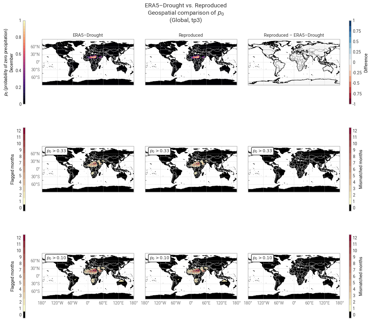
Fig. 6.1.6 Global probability of zero precipitation in the 3-month accumulation period and associated masks in ERA5–Drought (left) vs. reproduced from ERA5 precipitation data (middle) and the difference or mismatch between the two (right). Probability is displayed for one calendar month (December) across the reference window (1991–2020). Masks are displayed as the number of calendar months that get flagged and the oceans are masked, following [Keune+25] Fig. 3.

Example region, 1-month

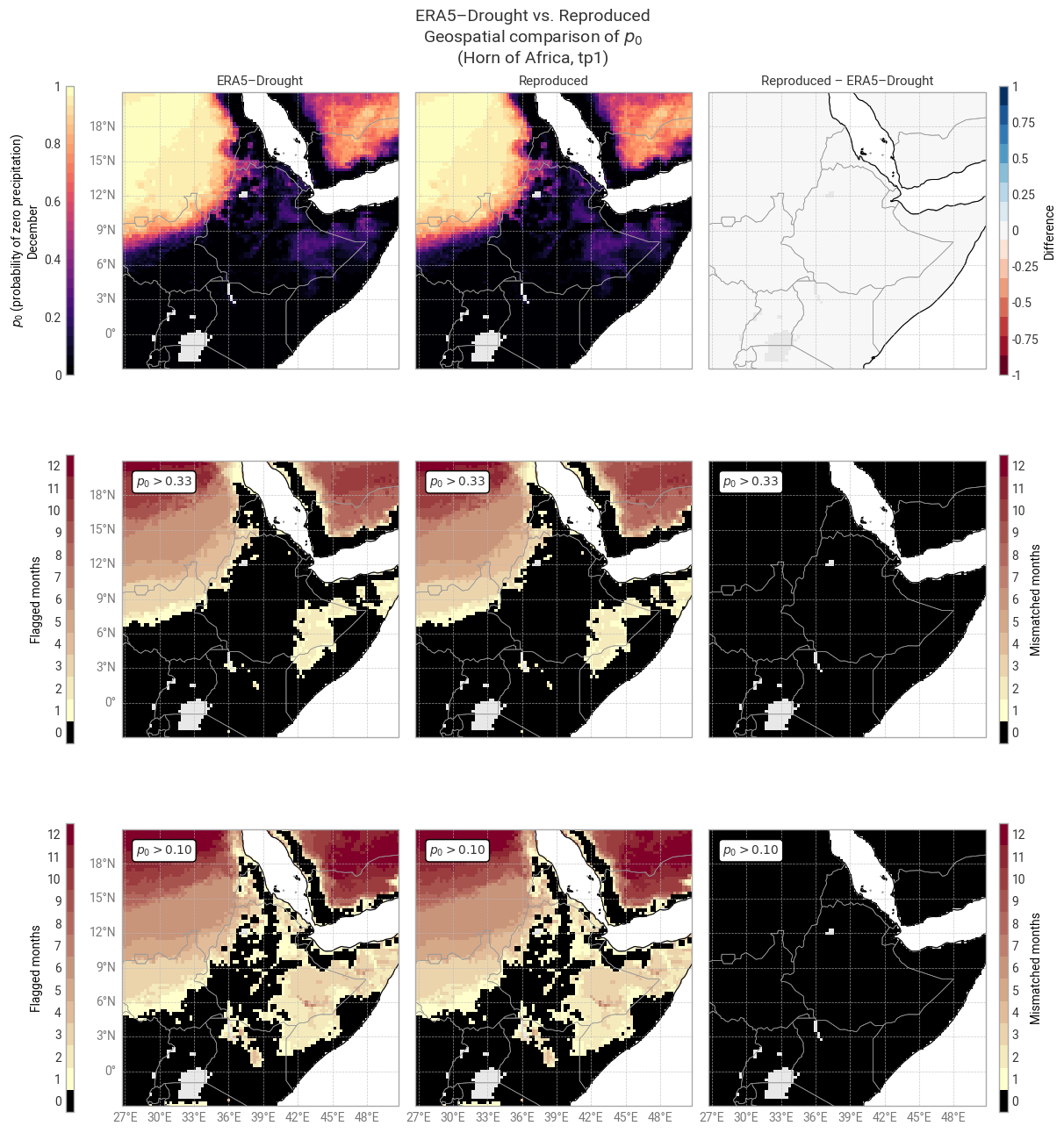
Fig. 6.1.7 Probability of zero precipitation in the 1-month accumulation period and associated masks in ERA5–Drought (left) vs. reproduced from ERA5 precipitation data (middle) and the difference or mismatch between the two (right). Probability is displayed for one calendar month (December) across the reference window (1991–2020). Masks are displayed as the number of calendar months that get flagged and the oceans are masked, following [Keune+25] Fig. 3. This figure displays only the example region (Horn of Africa), for comparison with Figure 6.1.4.

3.9 Quality flags: Shapiro–Wilk normality test

Another quality flag included in ERA5–Drought is the normality α, derived using the Shapiro–Wilk test [Shapiro+65]. This α quantifies how well the computed SPI or SPEI values in the reference period (1991–2020) are described by a standard normal distribution. As such, α is provided for each combination of calendar month and accumulation window, for each pixel. The mask in ERA–Drought uses a threshold of 0.05, meaning points where α < 0.05 are rejected.

In this subsection, we reproduce the α quality flag mask, and compare its values to those provided in ERA5–Drought. Because this involves computing SPI, which is computationally expensive, the evaluation is performed over the example region (Horn of Africa) rather than globally.

Show code cell source

Hide code cell source

# Select only desired site
data_era5_precipitation_region = data_era5_precipitation_preprocessed.sel(**example_region)

# Calculate SPI
spi_reproduced_region = calculate_spi_from_era5(data_era5_precipitation_region, reference_window=reference_window,
                                                evaluation_window=reference_window)

Show code cell source

Hide code cell source

# Apply Shapiro–Wilk normality test
normality_reproduced = shapiro_wilk_normality(spi_reproduced_region)

# Retain in memory
normality_reproduced = normality_reproduced.persist()

# Create mask from normality p-values
# True: above threshold, allowed
# False: below threshold, flagged
normality_reproduced_mask = (normality_reproduced >= 0.05)

# Display result
normality_reproduced_mask

Show code cell output

Hide code cell output

<xarray.Dataset> Size: 792kB
Dimensions:  (lat: 97, lon: 97, month: 12)
Coordinates:
    number   int64 8B 0
  * lat      (lat) float64 776B 21.0 20.75 20.5 20.25 ... -2.25 -2.5 -2.75 -3.0
  * lon      (lon) float64 776B 26.75 27.0 27.25 27.5 ... 50.0 50.25 50.5 50.75
  * month    (month) int64 96B 1 2 3 4 5 6 7 8 9 10 11 12
Data variables:
    SPI1     (month, lat, lon) bool 113kB dask.array<chunksize=(1, 33, 97), meta=np.ndarray>
    SPI3     (month, lat, lon) bool 113kB dask.array<chunksize=(1, 33, 97), meta=np.ndarray>
    SPI6     (month, lat, lon) bool 113kB dask.array<chunksize=(1, 33, 97), meta=np.ndarray>
    SPI12    (month, lat, lon) bool 113kB dask.array<chunksize=(1, 33, 97), meta=np.ndarray>
    SPI24    (month, lat, lon) bool 113kB dask.array<chunksize=(1, 33, 97), meta=np.ndarray>
    SPI36    (month, lat, lon) bool 113kB dask.array<chunksize=(1, 33, 97), meta=np.ndarray>
    SPI48    (month, lat, lon) bool 113kB dask.array<chunksize=(1, 33, 97), meta=np.ndarray>

xarray.Dataset

• Dimensions:
  • lat: 97
  • lon: 97
  • month: 12
• Coordinates: (4)
  • number
    ()
    int64
    0

    array(0)

  • lat
    (lat)
    float64
    21.0 20.75 20.5 ... -2.5 -2.75 -3.0

    array([21.  , 20.75, 20.5 , 20.25, 20.  , 19.75, 19.5 , 19.25, 19.  , 18.75,
           18.5 , 18.25, 18.  , 17.75, 17.5 , 17.25, 17.  , 16.75, 16.5 , 16.25,
           16.  , 15.75, 15.5 , 15.25, 15.  , 14.75, 14.5 , 14.25, 14.  , 13.75,
           13.5 , 13.25, 13.  , 12.75, 12.5 , 12.25, 12.  , 11.75, 11.5 , 11.25,
           11.  , 10.75, 10.5 , 10.25, 10.  ,  9.75,  9.5 ,  9.25,  9.  ,  8.75,
            8.5 ,  8.25,  8.  ,  7.75,  7.5 ,  7.25,  7.  ,  6.75,  6.5 ,  6.25,
            6.  ,  5.75,  5.5 ,  5.25,  5.  ,  4.75,  4.5 ,  4.25,  4.  ,  3.75,
            3.5 ,  3.25,  3.  ,  2.75,  2.5 ,  2.25,  2.  ,  1.75,  1.5 ,  1.25,
            1.  ,  0.75,  0.5 ,  0.25,  0.  , -0.25, -0.5 , -0.75, -1.  , -1.25,
           -1.5 , -1.75, -2.  , -2.25, -2.5 , -2.75, -3.  ])

  • lon
    (lon)
    float64
    26.75 27.0 27.25 ... 50.5 50.75

    array([26.75, 27.  , 27.25, 27.5 , 27.75, 28.  , 28.25, 28.5 , 28.75, 29.  ,
           29.25, 29.5 , 29.75, 30.  , 30.25, 30.5 , 30.75, 31.  , 31.25, 31.5 ,
           31.75, 32.  , 32.25, 32.5 , 32.75, 33.  , 33.25, 33.5 , 33.75, 34.  ,
           34.25, 34.5 , 34.75, 35.  , 35.25, 35.5 , 35.75, 36.  , 36.25, 36.5 ,
           36.75, 37.  , 37.25, 37.5 , 37.75, 38.  , 38.25, 38.5 , 38.75, 39.  ,
           39.25, 39.5 , 39.75, 40.  , 40.25, 40.5 , 40.75, 41.  , 41.25, 41.5 ,
           41.75, 42.  , 42.25, 42.5 , 42.75, 43.  , 43.25, 43.5 , 43.75, 44.  ,
           44.25, 44.5 , 44.75, 45.  , 45.25, 45.5 , 45.75, 46.  , 46.25, 46.5 ,
           46.75, 47.  , 47.25, 47.5 , 47.75, 48.  , 48.25, 48.5 , 48.75, 49.  ,
           49.25, 49.5 , 49.75, 50.  , 50.25, 50.5 , 50.75])

  • month
    (month)
    int64
    1 2 3 4 5 6 7 8 9 10 11 12

    long_name :

    time

    standard_name :

    time

    array([ 1,  2,  3,  4,  5,  6,  7,  8,  9, 10, 11, 12])

• Data variables: (7)
  • SPI1
    (month, lat, lon)
    bool
    dask.array<chunksize=(1, 33, 97), meta=np.ndarray>

    Array Chunk Bytes 110.26 kiB 6.06 kiB Shape (12, 97, 97) (1, 64, 97) Dask graph 24 chunks in 2 graph layers Data type bool numpy.ndarray

  • SPI3
    (month, lat, lon)
    bool
    dask.array<chunksize=(1, 33, 97), meta=np.ndarray>

    Array Chunk Bytes 110.26 kiB 6.06 kiB Shape (12, 97, 97) (1, 64, 97) Dask graph 24 chunks in 2 graph layers Data type bool numpy.ndarray

  • SPI6
    (month, lat, lon)
    bool
    dask.array<chunksize=(1, 33, 97), meta=np.ndarray>

    Array Chunk Bytes 110.26 kiB 6.06 kiB Shape (12, 97, 97) (1, 64, 97) Dask graph 24 chunks in 2 graph layers Data type bool numpy.ndarray

  • SPI12
    (month, lat, lon)
    bool
    dask.array<chunksize=(1, 33, 97), meta=np.ndarray>

    Array Chunk Bytes 110.26 kiB 6.06 kiB Shape (12, 97, 97) (1, 64, 97) Dask graph 24 chunks in 2 graph layers Data type bool numpy.ndarray

  • SPI24
    (month, lat, lon)
    bool
    dask.array<chunksize=(1, 33, 97), meta=np.ndarray>

    Array Chunk Bytes 110.26 kiB 6.06 kiB Shape (12, 97, 97) (1, 64, 97) Dask graph 24 chunks in 2 graph layers Data type bool numpy.ndarray

  • SPI36
    (month, lat, lon)
    bool
    dask.array<chunksize=(1, 33, 97), meta=np.ndarray>

    Array Chunk Bytes 110.26 kiB 6.06 kiB Shape (12, 97, 97) (1, 64, 97) Dask graph 24 chunks in 2 graph layers Data type bool numpy.ndarray

  • SPI48
    (month, lat, lon)
    bool
    dask.array<chunksize=(1, 33, 97), meta=np.ndarray>

    Array Chunk Bytes 110.26 kiB 6.06 kiB Shape (12, 97, 97) (1, 64, 97) Dask graph 24 chunks in 2 graph layers Data type bool numpy.ndarray

• Indexes: (3)
  • lat
    PandasIndex

    PandasIndex(Index([ 21.0, 20.75,  20.5, 20.25,  20.0, 19.75,  19.5, 19.25,  19.0, 18.75,
            18.5, 18.25,  18.0, 17.75,  17.5, 17.25,  17.0, 16.75,  16.5, 16.25,
            16.0, 15.75,  15.5, 15.25,  15.0, 14.75,  14.5, 14.25,  14.0, 13.75,
            13.5, 13.25,  13.0, 12.75,  12.5, 12.25,  12.0, 11.75,  11.5, 11.25,
            11.0, 10.75,  10.5, 10.25,  10.0,  9.75,   9.5,  9.25,   9.0,  8.75,
             8.5,  8.25,   8.0,  7.75,   7.5,  7.25,   7.0,  6.75,   6.5,  6.25,
             6.0,  5.75,   5.5,  5.25,   5.0,  4.75,   4.5,  4.25,   4.0,  3.75,
             3.5,  3.25,   3.0,  2.75,   2.5,  2.25,   2.0,  1.75,   1.5,  1.25,
             1.0,  0.75,   0.5,  0.25,   0.0, -0.25,  -0.5, -0.75,  -1.0, -1.25,
            -1.5, -1.75,  -2.0, -2.25,  -2.5, -2.75,  -3.0],
          dtype='float64', name='lat'))

  • lon
    PandasIndex

    PandasIndex(Index([26.75,  27.0, 27.25,  27.5, 27.75,  28.0, 28.25,  28.5, 28.75,  29.0,
           29.25,  29.5, 29.75,  30.0, 30.25,  30.5, 30.75,  31.0, 31.25,  31.5,
           31.75,  32.0, 32.25,  32.5, 32.75,  33.0, 33.25,  33.5, 33.75,  34.0,
           34.25,  34.5, 34.75,  35.0, 35.25,  35.5, 35.75,  36.0, 36.25,  36.5,
           36.75,  37.0, 37.25,  37.5, 37.75,  38.0, 38.25,  38.5, 38.75,  39.0,
           39.25,  39.5, 39.75,  40.0, 40.25,  40.5, 40.75,  41.0, 41.25,  41.5,
           41.75,  42.0, 42.25,  42.5, 42.75,  43.0, 43.25,  43.5, 43.75,  44.0,
           44.25,  44.5, 44.75,  45.0, 45.25,  45.5, 45.75,  46.0, 46.25,  46.5,
           46.75,  47.0, 47.25,  47.5, 47.75,  48.0, 48.25,  48.5, 48.75,  49.0,
           49.25,  49.5, 49.75,  50.0, 50.25,  50.5, 50.75],
          dtype='float64', name='lon'))

  • month
    PandasIndex

    PandasIndex(Index([1, 2, 3, 4, 5, 6, 7, 8, 9, 10, 11, 12], dtype='int64', name='month'))

• Attributes: (0)

The CDS provides ERA5–Drought’s α flag for each accumulation period, but does not distinguish between them in the variable name. This means that α must be downloaded separately for each accumulation period, renamed, and merged together, rather than downloading it for all simultaneously. Note that unlike for p₀, ERA5–Drought does not provide the value of α, only the corresponding boolean mask.

Show code cell source

Hide code cell source

# Setup: Request for each accumulation period
request_normality = {
    "variable": ["test_for_normality_spi"],
} | request_region | request_era5drought_flag

requests_per_accumulation_period = {period: {"accumulation_period": [str(period)],}
                                    for period in ACCUMULATION_PERIODS}

subrequests_era5drought_normality = {period: (req | request_normality)
                                       for period, req in requests_per_accumulation_period.items()}

# Download data in individual requests
normality_era5drought_mask = {period: ekd.from_source("cds", ID_ERA5_DROUGHT, subreq)  # Download as field lists
                              for period, subreq in subrequests_era5drought_normality.items()}

# Pre-process: Convert to xarray, handle variable names, month dimension
normality_era5drought_mask = preprocess_era5drought_qualityflag(normality_era5drought_mask, "SPI")
normality_era5drought_mask = normality_era5drought_mask.astype(bool)  # Convert to boolean array (values are only 0. or 1.)

# Display in notebook
normality_era5drought_mask

Show code cell output

Hide code cell output

<xarray.Dataset> Size: 792kB
Dimensions:  (month: 12, lat: 97, lon: 97)
Coordinates:
    time     (month) datetime64[ns] 96B 2020-01-01 2020-02-01 ... 2020-12-01
  * lon      (lon) float64 776B 26.75 27.0 27.25 27.5 ... 50.0 50.25 50.5 50.75
  * lat      (lat) float64 776B 21.0 20.75 20.5 20.25 ... -2.25 -2.5 -2.75 -3.0
  * month    (month) int64 96B 1 2 3 4 5 6 7 8 9 10 11 12
Data variables:
    SPI1     (month, lat, lon) bool 113kB dask.array<chunksize=(1, 97, 97), meta=np.ndarray>
    SPI3     (month, lat, lon) bool 113kB dask.array<chunksize=(1, 97, 97), meta=np.ndarray>
    SPI6     (month, lat, lon) bool 113kB dask.array<chunksize=(1, 97, 97), meta=np.ndarray>
    SPI12    (month, lat, lon) bool 113kB dask.array<chunksize=(1, 97, 97), meta=np.ndarray>
    SPI24    (month, lat, lon) bool 113kB dask.array<chunksize=(1, 97, 97), meta=np.ndarray>
    SPI36    (month, lat, lon) bool 113kB dask.array<chunksize=(1, 97, 97), meta=np.ndarray>
    SPI48    (month, lat, lon) bool 113kB dask.array<chunksize=(1, 97, 97), meta=np.ndarray>
Attributes: (12/19)
    CDI:                     Climate Data Interface version 1.9.10 (https://m...
    Conventions:             CF-1.8
    source:                  DRYFALL v1.0
    institution:             European Centre for Medium-Range Weather Forecasts
    title:                   Quality criteria for the derived standardized dr...
    description:             Monthly quality criteria that define the reliabi...
    ...                      ...
    resolution:              0.25x0.25
    climate_start_date:      1991-01-01
    climate_end_date:        2020-12-31
    frequency:               Monthly
    contact_person:          support@ecmwf.int
    CDO:                     Climate Data Operators version 1.9.10 (https://m...

xarray.Dataset

• Dimensions:
  • month: 12
  • lat: 97
  • lon: 97
• Coordinates: (4)
  • time
    (month)
    datetime64[ns]
    2020-01-01 ... 2020-12-01

    standard_name :

    time

    axis :

    T

    array(['2020-01-01T00:00:00.000000000', '2020-02-01T00:00:00.000000000',
           '2020-03-01T00:00:00.000000000', '2020-04-01T00:00:00.000000000',
           '2020-05-01T00:00:00.000000000', '2020-06-01T00:00:00.000000000',
           '2020-07-01T00:00:00.000000000', '2020-08-01T00:00:00.000000000',
           '2020-09-01T00:00:00.000000000', '2020-10-01T00:00:00.000000000',
           '2020-11-01T00:00:00.000000000', '2020-12-01T00:00:00.000000000'],
          dtype='datetime64[ns]')

  • lon
    (lon)
    float64
    26.75 27.0 27.25 ... 50.5 50.75

    standard_name :

    longitude

    long_name :

    longitude

    units :

    degrees_east

    axis :

    X

    array([26.75, 27.  , 27.25, 27.5 , 27.75, 28.  , 28.25, 28.5 , 28.75, 29.  ,
           29.25, 29.5 , 29.75, 30.  , 30.25, 30.5 , 30.75, 31.  , 31.25, 31.5 ,
           31.75, 32.  , 32.25, 32.5 , 32.75, 33.  , 33.25, 33.5 , 33.75, 34.  ,
           34.25, 34.5 , 34.75, 35.  , 35.25, 35.5 , 35.75, 36.  , 36.25, 36.5 ,
           36.75, 37.  , 37.25, 37.5 , 37.75, 38.  , 38.25, 38.5 , 38.75, 39.  ,
           39.25, 39.5 , 39.75, 40.  , 40.25, 40.5 , 40.75, 41.  , 41.25, 41.5 ,
           41.75, 42.  , 42.25, 42.5 , 42.75, 43.  , 43.25, 43.5 , 43.75, 44.  ,
           44.25, 44.5 , 44.75, 45.  , 45.25, 45.5 , 45.75, 46.  , 46.25, 46.5 ,
           46.75, 47.  , 47.25, 47.5 , 47.75, 48.  , 48.25, 48.5 , 48.75, 49.  ,
           49.25, 49.5 , 49.75, 50.  , 50.25, 50.5 , 50.75])

  • lat
    (lat)
    float64
    21.0 20.75 20.5 ... -2.5 -2.75 -3.0

    standard_name :

    latitude

    long_name :

    latitude

    units :

    degrees_north

    axis :

    Y

    array([21.  , 20.75, 20.5 , 20.25, 20.  , 19.75, 19.5 , 19.25, 19.  , 18.75,
           18.5 , 18.25, 18.  , 17.75, 17.5 , 17.25, 17.  , 16.75, 16.5 , 16.25,
           16.  , 15.75, 15.5 , 15.25, 15.  , 14.75, 14.5 , 14.25, 14.  , 13.75,
           13.5 , 13.25, 13.  , 12.75, 12.5 , 12.25, 12.  , 11.75, 11.5 , 11.25,
           11.  , 10.75, 10.5 , 10.25, 10.  ,  9.75,  9.5 ,  9.25,  9.  ,  8.75,
            8.5 ,  8.25,  8.  ,  7.75,  7.5 ,  7.25,  7.  ,  6.75,  6.5 ,  6.25,
            6.  ,  5.75,  5.5 ,  5.25,  5.  ,  4.75,  4.5 ,  4.25,  4.  ,  3.75,
            3.5 ,  3.25,  3.  ,  2.75,  2.5 ,  2.25,  2.  ,  1.75,  1.5 ,  1.25,
            1.  ,  0.75,  0.5 ,  0.25,  0.  , -0.25, -0.5 , -0.75, -1.  , -1.25,
           -1.5 , -1.75, -2.  , -2.25, -2.5 , -2.75, -3.  ])

  • month
    (month)
    int64
    1 2 3 4 5 6 7 8 9 10 11 12

    standard_name :

    time

    axis :

    T

    array([ 1,  2,  3,  4,  5,  6,  7,  8,  9, 10, 11, 12])

• Data variables: (7)
  • SPI1
    (month, lat, lon)
    bool
    dask.array<chunksize=(1, 97, 97), meta=np.ndarray>

    long_name :

    Quality flag that indicates the acceptance of a Shapiro-Wilks test for normality using the derived standardized indices during the reference period; 1 indicates significant values and 0 indicates non-significant values at the alpha=0.05 level.

    units :

    1

    Array Chunk Bytes 110.26 kiB 9.19 kiB Shape (12, 97, 97) (1, 97, 97) Dask graph 12 chunks in 26 graph layers Data type bool numpy.ndarray

  • SPI3
    (month, lat, lon)
    bool
    dask.array<chunksize=(1, 97, 97), meta=np.ndarray>

    long_name :

    Quality flag that indicates the acceptance of a Shapiro-Wilks test for normality using the derived standardized indices during the reference period; 1 indicates significant values and 0 indicates non-significant values at the alpha=0.05 level.

    units :

    1

    Array Chunk Bytes 110.26 kiB 9.19 kiB Shape (12, 97, 97) (1, 97, 97) Dask graph 12 chunks in 26 graph layers Data type bool numpy.ndarray

  • SPI6
    (month, lat, lon)
    bool
    dask.array<chunksize=(1, 97, 97), meta=np.ndarray>

    long_name :

    Quality flag that indicates the acceptance of a Shapiro-Wilks test for normality using the derived standardized indices during the reference period; 1 indicates significant values and 0 indicates non-significant values at the alpha=0.05 level.

    units :

    1

    Array Chunk Bytes 110.26 kiB 9.19 kiB Shape (12, 97, 97) (1, 97, 97) Dask graph 12 chunks in 26 graph layers Data type bool numpy.ndarray

  • SPI12
    (month, lat, lon)
    bool
    dask.array<chunksize=(1, 97, 97), meta=np.ndarray>

    long_name :

    Quality flag that indicates the acceptance of a Shapiro-Wilks test for normality using the derived standardized indices during the reference period; 1 indicates significant values and 0 indicates non-significant values at the alpha=0.05 level.

    units :

    1

    Array Chunk Bytes 110.26 kiB 9.19 kiB Shape (12, 97, 97) (1, 97, 97) Dask graph 12 chunks in 26 graph layers Data type bool numpy.ndarray

  • SPI24
    (month, lat, lon)
    bool
    dask.array<chunksize=(1, 97, 97), meta=np.ndarray>

    long_name :

    Quality flag that indicates the acceptance of a Shapiro-Wilks test for normality using the derived standardized indices during the reference period; 1 indicates significant values and 0 indicates non-significant values at the alpha=0.05 level.

    units :

    1

    Array Chunk Bytes 110.26 kiB 9.19 kiB Shape (12, 97, 97) (1, 97, 97) Dask graph 12 chunks in 26 graph layers Data type bool numpy.ndarray

  • SPI36
    (month, lat, lon)
    bool
    dask.array<chunksize=(1, 97, 97), meta=np.ndarray>

    long_name :

    Quality flag that indicates the acceptance of a Shapiro-Wilks test for normality using the derived standardized indices during the reference period; 1 indicates significant values and 0 indicates non-significant values at the alpha=0.05 level.

    units :

    1

    Array Chunk Bytes 110.26 kiB 9.19 kiB Shape (12, 97, 97) (1, 97, 97) Dask graph 12 chunks in 26 graph layers Data type bool numpy.ndarray

  • SPI48
    (month, lat, lon)
    bool
    dask.array<chunksize=(1, 97, 97), meta=np.ndarray>

    long_name :

    Quality flag that indicates the acceptance of a Shapiro-Wilks test for normality using the derived standardized indices during the reference period; 1 indicates significant values and 0 indicates non-significant values at the alpha=0.05 level.

    units :

    1

    Array Chunk Bytes 110.26 kiB 9.19 kiB Shape (12, 97, 97) (1, 97, 97) Dask graph 12 chunks in 26 graph layers Data type bool numpy.ndarray

• Indexes: (3)
  • lon
    PandasIndex

    PandasIndex(Index([26.75,  27.0, 27.25,  27.5, 27.75,  28.0, 28.25,  28.5, 28.75,  29.0,
           29.25,  29.5, 29.75,  30.0, 30.25,  30.5, 30.75,  31.0, 31.25,  31.5,
           31.75,  32.0, 32.25,  32.5, 32.75,  33.0, 33.25,  33.5, 33.75,  34.0,
           34.25,  34.5, 34.75,  35.0, 35.25,  35.5, 35.75,  36.0, 36.25,  36.5,
           36.75,  37.0, 37.25,  37.5, 37.75,  38.0, 38.25,  38.5, 38.75,  39.0,
           39.25,  39.5, 39.75,  40.0, 40.25,  40.5, 40.75,  41.0, 41.25,  41.5,
           41.75,  42.0, 42.25,  42.5, 42.75,  43.0, 43.25,  43.5, 43.75,  44.0,
           44.25,  44.5, 44.75,  45.0, 45.25,  45.5, 45.75,  46.0, 46.25,  46.5,
           46.75,  47.0, 47.25,  47.5, 47.75,  48.0, 48.25,  48.5, 48.75,  49.0,
           49.25,  49.5, 49.75,  50.0, 50.25,  50.5, 50.75],
          dtype='float64', name='lon'))

  • lat
    PandasIndex

    PandasIndex(Index([ 21.0, 20.75,  20.5, 20.25,  20.0, 19.75,  19.5, 19.25,  19.0, 18.75,
            18.5, 18.25,  18.0, 17.75,  17.5, 17.25,  17.0, 16.75,  16.5, 16.25,
            16.0, 15.75,  15.5, 15.25,  15.0, 14.75,  14.5, 14.25,  14.0, 13.75,
            13.5, 13.25,  13.0, 12.75,  12.5, 12.25,  12.0, 11.75,  11.5, 11.25,
            11.0, 10.75,  10.5, 10.25,  10.0,  9.75,   9.5,  9.25,   9.0,  8.75,
             8.5,  8.25,   8.0,  7.75,   7.5,  7.25,   7.0,  6.75,   6.5,  6.25,
             6.0,  5.75,   5.5,  5.25,   5.0,  4.75,   4.5,  4.25,   4.0,  3.75,
             3.5,  3.25,   3.0,  2.75,   2.5,  2.25,   2.0,  1.75,   1.5,  1.25,
             1.0,  0.75,   0.5,  0.25,   0.0, -0.25,  -0.5, -0.75,  -1.0, -1.25,
            -1.5, -1.75,  -2.0, -2.25,  -2.5, -2.75,  -3.0],
          dtype='float64', name='lat'))

  • month
    PandasIndex

    PandasIndex(Index([1, 2, 3, 4, 5, 6, 7, 8, 9, 10, 11, 12], dtype='int64', name='month'))

• Attributes: (19)

  CDI :

  Climate Data Interface version 1.9.10 (https://mpimet.mpg.de/cdi)

  Conventions :

  CF-1.8

  source :

  DRYFALL v1.0

  institution :

  European Centre for Medium-Range Weather Forecasts

  title :

  Quality criteria for the derived standardized drought indices

  description :

  Monthly quality criteria that define the reliability of the derived drought indices.

  history :

  Tue Aug 13 11:21:46 2024: cdo -selvar,significance -setdate,20200101 -seldate,19000101 /ec/ws4/tc/emos/work/cems/dryfall/emos/dryfall_monthly/generated_climate/parameters/SPI1_gamma_global_era5_moda_ref1991to2020_params.nc SPI1_spisignificance_gamma_global_era5_moda_ref1991to2020_01.nc Created 13/08/2024 11:10:50 using DRYFALL.

  license :

  Creative Commons Attribution v4

  citation_statement :

  Drought indicators derived from ERA5 reanalysis

  ref_publication :

  Keune, J., F. Di Giuseppe, C. Barnard, D. Damasio da Costa, and F. Wetterhall: ERA5–Drought: Global drought indicators based on ECMWF reanalysis.

  cds_data_catalogue_url :

  https://ecds.climate.copernicus.eu/datasets/derived-drought-historical

  data_srs :

  EPSG:4326

  extent :

  -180,-90,180,90

  resolution :

  0.25x0.25

  climate_start_date :

  1991-01-01

  climate_end_date :

  2020-12-31

  frequency :

  Monthly

  contact_person :

  support@ecmwf.int

  CDO :

  Climate Data Operators version 1.9.10 (https://mpimet.mpg.de/cdo)

First, we quantitatively compare how often the values of the normality mask desired from α in ERA5–Drought and the reproduction match:

Show code cell source

Hide code cell source

# Package probability and masks into dictionary for table function; note use unicode symbols / HTML
normality_flags = {"α < 0.05 [%]": [normality_reproduced_mask, normality_era5drought_mask],
                  }

# Compare probabilities per variable
compare_quality_flags(normality_flags, title_suffix=f" ({domain_region.name})")

ERA5–Drought vs. Reproduced Quality flag matches (Horn of Africa)

	SPI-1	SPI-3	SPI-6	SPI-12	SPI-24	SPI-36	SPI-48
Matching α < 0.05 [%]	74.83	84.23	87.91	92.21	90.39	90.06	88.80

The table above shows good agreement, especially for longer accumulation periods. For SPI-1, a quarter of the comparisons do not match. While there are pixels across the entire region where α does not match for one or two calendar months (Figure 6.1.8), the majority of mismatches are concentrated in deserts (Sahara and Arabian peninsula), which in practice would be masked anyway for failing the p₀ test (see above). This pattern is even stronger in the distribution of SPI-3 normality (Figure 6.1.9). It is more difficult to fit a gamma distribution in drier areas and drier calendar months, in which case SPI values are less trustworthy – meaning the normality flag is working as intended.

In conclusion, the differences in the normality mask (α < 0.05) seen above are likely caused by the differences in fitted distributions seen before, and thus do not affect the assessment of reproducibility. The mask provided with ERA5–Drought can be used confidently to mask corresponding SPI values.

Show code cell source

Hide code cell source

# Package masks into dictionary for plotting function; note use of LaTeX instead of unicode/HTML symbols
masks = {r"$\alpha < 0.05$": [normality_era5drought_mask, normality_reproduced_mask],
        }

# Display quality flags – this step may take a few minutes
# SPI-1: Compare to table
plot_geospatial_comparison_quality_flags("SPI1", masks=masks,
                                         shared_mask=LAND, domain=domain_region,
                                         glue_label="indicator_derived-drought-historical-monthly_consistency_q01_fig-spi-normality-region-spi1")

# SPI-3: Compare to Keune+25 Fig 3.
plot_geospatial_comparison_quality_flags("SPI3", masks=masks,
                                         shared_mask=LAND, domain=domain_region,
                                         glue_label="indicator_derived-drought-historical-monthly_consistency_q01_fig-spi-normality-region-spi3")

SPI-1

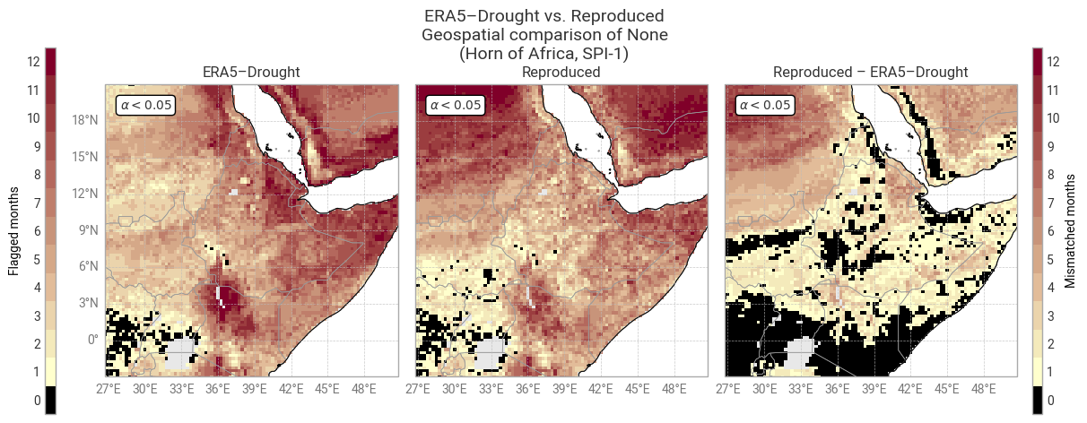
Fig. 6.1.8 Shapiro–Wilk normality α for SPI-1 and associated masks in ERA5–Drought (left) vs. reproduced from ERA5 precipitation data (middle) and the difference or mismatch between the two (right). The α < 0.05 mask is displayed as the number of calendar months that get flagged and the oceans are masked, following [Keune+25] Fig. 3. This figure displays only the example region (Horn of Africa).

SPI-3

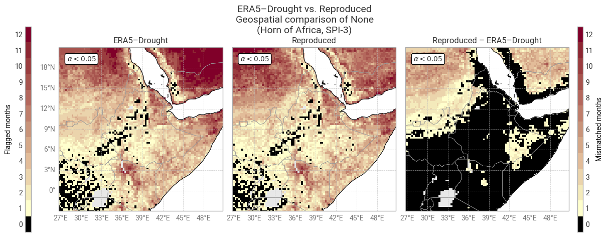
Fig. 6.1.9 Shapiro–Wilk normality α for SPI-3 and associated masks in ERA5–Drought (left) vs. reproduced from ERA5 precipitation data (middle) and the difference or mismatch between the two (right). The α < 0.05 mask is displayed as the number of calendar months that get flagged and the oceans are masked, following [Keune+25] Fig. 3. This figure displays only the example region (Horn of Africa).

4. SPEI comparison

The process of calculating SPEI is very similar to that for SPI, with three major differences:

• SPEI is based on the water balance (precipitation and potential evaporation or evapotranspiration), rather than just precipitation.

• SPEI is based on a logistic distribution, rather than a gamma distribution.

• SPEI does not need to be adjusted for months with zero precipitation.

As such, this section is structured similarly to 3. SPI comparison and can be run entirely independently, but some of the more detailed explanations from said section are left out for brevity this time.

4.1 Download monthly precipitation and potential evaporation data from ERA5

First, the monthly-mean total precipitation (variable 228.128) and evaporation (variable 251.228) are downloaded from the Complete ERA5 global atmospheric reanalysis dataset. More information about the format for these requests is available in the MARS ERA5 catalogue.

When executing this notebook yourself, if you have previously run 3. SPI comparison and have caching enabled in earthkit-data, the downloaded precipitation data will be re-used.

Show code cell source

Hide code cell source

request_era5_precipitation_moda = {
    "param": "228.128",  # Variable: Total precipitation
    "stream": "moda",    # Data stream: Monthly mean reanalysis
} | request_era5_template

request_era5_pev_moda = {
    "param": "251.228",  # Variable: Potential evaporation
    "stream": "moda",    # Data stream: Monthly mean reanalysis
} | request_era5_template

Show code cell source

Hide code cell source

# Download data and load into xarray
data_era5_waterbalance_cds = ekd.from_source("cds", ID_ERA5, request_era5_precipitation_moda, request_era5_pev_moda)  # Download as field list
data_era5_waterbalance_cds = data_era5_waterbalance_cds.to_xarray(compat="equals")  # Convert to xarray dataset

# Pre-process to desired format
# Note the change in variable name
data_era5_waterbalance_preprocessed = preprocess_era5(data_era5_waterbalance_cds)

# Display in notebook
data_era5_waterbalance_preprocessed

<xarray.Dataset> Size: 8GB
Dimensions:  (time: 1020, lat: 721, lon: 1440)
Coordinates:
    number   int64 8B 0
  * time     (time) datetime64[ns] 8kB 1940-01-01T06:00:00 ... 2024-12-01T06:...
  * lat      (lat) float64 6kB 90.0 89.75 89.5 89.25 ... -89.5 -89.75 -90.0
    expver   (time) <U4 16kB dask.array<chunksize=(1020,), meta=np.ndarray>
  * lon      (lon) float64 12kB -180.0 -179.8 -179.5 ... 179.2 179.5 179.8
Data variables:
    tp       (time, lat, lon) float32 4GB dask.array<chunksize=(1020, 103, 360), meta=np.ndarray>
    pev      (time, lat, lon) float32 4GB dask.array<chunksize=(1020, 103, 360), meta=np.ndarray>
Attributes:
    GRIB_centre:             ecmf
    GRIB_centreDescription:  European Centre for Medium-Range Weather Forecasts
    GRIB_subCentre:          0
    Conventions:             CF-1.7
    institution:             European Centre for Medium-Range Weather Forecasts

xarray.Dataset

• Dimensions:
  • time: 1020
  • lat: 721
  • lon: 1440
• Coordinates: (5)
  • number
    ()
    int64
    0

    long_name :

    ensemble member numerical id

    units :

    1

    standard_name :

    realization

    array(0)

  • time
    (time)
    datetime64[ns]
    1940-01-01T06:00:00 ... 2024-12-...

    long_name :

    time

    standard_name :

    time

    array(['1940-01-01T06:00:00.000000000', '1940-02-01T06:00:00.000000000',
           '1940-03-01T06:00:00.000000000', ..., '2024-10-01T06:00:00.000000000',
           '2024-11-01T06:00:00.000000000', '2024-12-01T06:00:00.000000000'],
          shape=(1020,), dtype='datetime64[ns]')

  • lat
    (lat)
    float64
    90.0 89.75 89.5 ... -89.75 -90.0

    units :

    degrees_north

    standard_name :

    latitude

    long_name :

    latitude

    stored_direction :

    decreasing

    array([ 90.  ,  89.75,  89.5 , ..., -89.5 , -89.75, -90.  ], shape=(721,))

  • expver
    (time)
    <U4
    dask.array<chunksize=(1020,), meta=np.ndarray>

    Array Chunk Bytes 15.94 kiB 15.94 kiB Shape (1020,) (1020,) Dask graph 1 chunks in 1 graph layer Data type

  • lon
    (lon)
    float64
    -180.0 -179.8 ... 179.5 179.8

    array([-180.  , -179.75, -179.5 , ...,  179.25,  179.5 ,  179.75],
          shape=(1440,))

• Data variables: (2)
  • tp
    (time, lat, lon)
    float32
    dask.array<chunksize=(1020, 103, 360), meta=np.ndarray>

    GRIB_paramId :

    228

    GRIB_dataType :

    fc

    GRIB_numberOfPoints :

    1038240

    GRIB_typeOfLevel :

    surface

    GRIB_stepUnits :

    1

    GRIB_stepType :

    avgad

    GRIB_gridType :

    regular_ll

    GRIB_uvRelativeToGrid :

    0

    GRIB_NV :

    0

    GRIB_Nx :

    1440

    GRIB_Ny :

    721

    GRIB_cfName :

    unknown

    GRIB_cfVarName :

    tp

    GRIB_gridDefinitionDescription :

    Latitude/Longitude Grid

    GRIB_iDirectionIncrementInDegrees :

    0.25

    GRIB_iScansNegatively :

    0

    GRIB_jDirectionIncrementInDegrees :

    0.25

    GRIB_jPointsAreConsecutive :

    0

    GRIB_jScansPositively :

    0

    GRIB_latitudeOfFirstGridPointInDegrees :

    90.0

    GRIB_latitudeOfLastGridPointInDegrees :

    -90.0

    GRIB_longitudeOfFirstGridPointInDegrees :

    0.0

    GRIB_longitudeOfLastGridPointInDegrees :

    359.75

    GRIB_missingValue :

    3.4028234663852886e+38

    GRIB_name :

    Total precipitation

    GRIB_shortName :

    tp

    GRIB_totalNumber :

    0

    GRIB_units :

    m

    long_name :

    Total precipitation

    units :

    mm

    standard_name :

    unknown

    GRIB_surface :

    0.0

    Array Chunk Bytes 3.95 GiB 144.28 MiB Shape (1020, 721, 1440) (1020, 103, 360) Dask graph 28 chunks in 5 graph layers Data type float32 numpy.ndarray

  • pev
    (time, lat, lon)
    float32
    dask.array<chunksize=(1020, 103, 360), meta=np.ndarray>

    GRIB_paramId :

    228251

    GRIB_dataType :

    fc

    GRIB_numberOfPoints :

    1038240

    GRIB_typeOfLevel :

    surface

    GRIB_stepUnits :

    1

    GRIB_stepType :

    avgad

    GRIB_gridType :

    regular_ll

    GRIB_uvRelativeToGrid :

    0

    GRIB_NV :

    0

    GRIB_Nx :

    1440

    GRIB_Ny :

    721

    GRIB_cfName :

    unknown

    GRIB_cfVarName :

    pev

    GRIB_gridDefinitionDescription :

    Latitude/Longitude Grid

    GRIB_iDirectionIncrementInDegrees :

    0.25

    GRIB_iScansNegatively :

    0

    GRIB_jDirectionIncrementInDegrees :

    0.25

    GRIB_jPointsAreConsecutive :

    0

    GRIB_jScansPositively :

    0

    GRIB_latitudeOfFirstGridPointInDegrees :

    90.0

    GRIB_latitudeOfLastGridPointInDegrees :

    -90.0

    GRIB_longitudeOfFirstGridPointInDegrees :

    0.0

    GRIB_longitudeOfLastGridPointInDegrees :

    359.75

    GRIB_missingValue :

    3.4028234663852886e+38

    GRIB_name :

    Potential evaporation

    GRIB_shortName :

    pev

    GRIB_totalNumber :

    0

    GRIB_units :

    m

    long_name :

    Potential evaporation

    units :

    mm

    standard_name :

    unknown

    GRIB_surface :

    0.0

    Array Chunk Bytes 3.95 GiB 144.28 MiB Shape (1020, 721, 1440) (1020, 103, 360) Dask graph 28 chunks in 5 graph layers Data type float32 numpy.ndarray

• Indexes: (3)
  • time
    PandasIndex

    PandasIndex(DatetimeIndex(['1940-01-01 06:00:00', '1940-02-01 06:00:00',
                   '1940-03-01 06:00:00', '1940-04-01 06:00:00',
                   '1940-05-01 06:00:00', '1940-06-01 06:00:00',
                   '1940-07-01 06:00:00', '1940-08-01 06:00:00',
                   '1940-09-01 06:00:00', '1940-10-01 06:00:00',
                   ...
                   '2024-03-01 06:00:00', '2024-04-01 06:00:00',
                   '2024-05-01 06:00:00', '2024-06-01 06:00:00',
                   '2024-07-01 06:00:00', '2024-08-01 06:00:00',
                   '2024-09-01 06:00:00', '2024-10-01 06:00:00',
                   '2024-11-01 06:00:00', '2024-12-01 06:00:00'],
                  dtype='datetime64[ns]', name='time', length=1020, freq=None))

  • lat
    PandasIndex

    PandasIndex(Index([  90.0,  89.75,   89.5,  89.25,   89.0,  88.75,   88.5,  88.25,   88.0,
            87.75,
           ...
           -87.75,  -88.0, -88.25,  -88.5, -88.75,  -89.0, -89.25,  -89.5, -89.75,
            -90.0],
          dtype='float64', name='lat', length=721))

  • lon
    PandasIndex

    PandasIndex(Index([ -180.0, -179.75,  -179.5, -179.25,  -179.0, -178.75,  -178.5, -178.25,
            -178.0, -177.75,
           ...
             177.5,  177.75,   178.0,  178.25,   178.5,  178.75,   179.0,  179.25,
             179.5,  179.75],
          dtype='float64', name='lon', length=1440))

• Attributes: (5)

  GRIB_centre :

  ecmf

  GRIB_centreDescription :

  European Centre for Medium-Range Weather Forecasts

  GRIB_subCentre :

  0

  Conventions :

  CF-1.7

  institution :

  European Centre for Medium-Range Weather Forecasts

4.2 Calculate water balance over accumulation periods

The water balance represents the net gain or loss of water in an area due to precipitation (gain) and evaporation (loss). ECMWF’s convention, as used in ERA5, is that downward fluxes are positive and upward fluxes are negative. This means that total precipitation is always positive (or zero), potential evaporation is always negative (or zero), and the water balance is simply the sum of the two: WB = TP + PEV.

Here, we calculate the water balance per point in the downloaded ERA5 data and accumulate it over the same periods as before (1, 3, 6, 12, 24, 36, and 48 months).

The resulting accumulated time series for the example site defined in 2. General setup, Addis Ababa in Ethiopia in our example, are displayed in Figure 6.1.10. This example clearly demonstrates how the water balance moves between positive and negative (net gain vs. net loss) and how this changes depending on the accumulation period. For example, the shortest accumulation periods (1–6 months) swing up and down seasonally, but the longer-term (e.g. 48-month) accumulated water balance tends to be positive except in specific periods (e.g. the 1960s).

Show code cell source

Hide code cell source

# Calculate water balance
data_era5_waterbalance = calculate_waterbalance(data_era5_waterbalance_preprocessed)

# Accumulate water balance
data_era5_waterbalance = accumulate(data_era5_waterbalance, "wb")

# Display result
data_era5_waterbalance

Show code cell output

Hide code cell output

<xarray.Dataset> Size: 59GB
Dimensions:  (time: 1020, lat: 721, lon: 1440)
Coordinates:
    number   int64 8B 0
  * time     (time) datetime64[ns] 8kB 1940-01-01T06:00:00 ... 2024-12-01T06:...
  * lat      (lat) float64 6kB 90.0 89.75 89.5 89.25 ... -89.5 -89.75 -90.0
    expver   (time) <U4 16kB dask.array<chunksize=(1020,), meta=np.ndarray>
  * lon      (lon) float64 12kB -180.0 -179.8 -179.5 ... 179.2 179.5 179.8
Data variables:
    wb1      (time, lat, lon) float64 8GB dask.array<chunksize=(1020, 103, 360), meta=np.ndarray>
    wb3      (time, lat, lon) float64 8GB dask.array<chunksize=(1020, 103, 360), meta=np.ndarray>
    wb6      (time, lat, lon) float64 8GB dask.array<chunksize=(1020, 103, 360), meta=np.ndarray>
    wb12     (time, lat, lon) float64 8GB dask.array<chunksize=(1020, 103, 360), meta=np.ndarray>
    wb24     (time, lat, lon) float64 8GB dask.array<chunksize=(1020, 103, 360), meta=np.ndarray>
    wb36     (time, lat, lon) float64 8GB dask.array<chunksize=(1020, 103, 360), meta=np.ndarray>
    wb48     (time, lat, lon) float64 8GB dask.array<chunksize=(1020, 103, 360), meta=np.ndarray>

xarray.Dataset

• Dimensions:
  • time: 1020
  • lat: 721
  • lon: 1440
• Coordinates: (5)
  • number
    ()
    int64
    0

    long_name :

    ensemble member numerical id

    units :

    1

    standard_name :

    realization

    array(0)

  • time
    (time)
    datetime64[ns]
    1940-01-01T06:00:00 ... 2024-12-...

    long_name :

    time

    standard_name :

    time

    array(['1940-01-01T06:00:00.000000000', '1940-02-01T06:00:00.000000000',
           '1940-03-01T06:00:00.000000000', ..., '2024-10-01T06:00:00.000000000',
           '2024-11-01T06:00:00.000000000', '2024-12-01T06:00:00.000000000'],
          shape=(1020,), dtype='datetime64[ns]')

  • lat
    (lat)
    float64
    90.0 89.75 89.5 ... -89.75 -90.0

    units :

    degrees_north

    standard_name :

    latitude

    long_name :

    latitude

    stored_direction :

    decreasing

    array([ 90.  ,  89.75,  89.5 , ..., -89.5 , -89.75, -90.  ], shape=(721,))

  • expver
    (time)
    <U4
    dask.array<chunksize=(1020,), meta=np.ndarray>

    Array Chunk Bytes 15.94 kiB 15.94 kiB Shape (1020,) (1020,) Dask graph 1 chunks in 1 graph layer Data type

  • lon
    (lon)
    float64
    -180.0 -179.8 ... 179.5 179.8

    array([-180.  , -179.75, -179.5 , ...,  179.25,  179.5 ,  179.75],
          shape=(1440,))

• Data variables: (7)
  • wb1
    (time, lat, lon)
    float64
    dask.array<chunksize=(1020, 103, 360), meta=np.ndarray>

    Array Chunk Bytes 7.89 GiB 288.56 MiB Shape (1020, 721, 1440) (1020, 103, 360) Dask graph 28 chunks in 26 graph layers Data type float64 numpy.ndarray

  • wb3
    (time, lat, lon)
    float64
    dask.array<chunksize=(1020, 103, 360), meta=np.ndarray>

    Array Chunk Bytes 7.89 GiB 288.56 MiB Shape (1020, 721, 1440) (1020, 103, 360) Dask graph 28 chunks in 36 graph layers Data type float64 numpy.ndarray

  • wb6
    (time, lat, lon)
    float64
    dask.array<chunksize=(1020, 103, 360), meta=np.ndarray>

    Array Chunk Bytes 7.89 GiB 288.56 MiB Shape (1020, 721, 1440) (1020, 103, 360) Dask graph 28 chunks in 36 graph layers Data type float64 numpy.ndarray

  • wb12
    (time, lat, lon)
    float64
    dask.array<chunksize=(1020, 103, 360), meta=np.ndarray>

    Array Chunk Bytes 7.89 GiB 288.56 MiB Shape (1020, 721, 1440) (1020, 103, 360) Dask graph 28 chunks in 36 graph layers Data type float64 numpy.ndarray

  • wb24
    (time, lat, lon)
    float64
    dask.array<chunksize=(1020, 103, 360), meta=np.ndarray>

    Array Chunk Bytes 7.89 GiB 288.56 MiB Shape (1020, 721, 1440) (1020, 103, 360) Dask graph 28 chunks in 36 graph layers Data type float64 numpy.ndarray

  • wb36
    (time, lat, lon)
    float64
    dask.array<chunksize=(1020, 103, 360), meta=np.ndarray>

    Array Chunk Bytes 7.89 GiB 288.56 MiB Shape (1020, 721, 1440) (1020, 103, 360) Dask graph 28 chunks in 36 graph layers Data type float64 numpy.ndarray

  • wb48
    (time, lat, lon)
    float64
    dask.array<chunksize=(1020, 103, 360), meta=np.ndarray>

    Array Chunk Bytes 7.89 GiB 288.56 MiB Shape (1020, 721, 1440) (1020, 103, 360) Dask graph 28 chunks in 36 graph layers Data type float64 numpy.ndarray

• Indexes: (3)
  • time
    PandasIndex

    PandasIndex(DatetimeIndex(['1940-01-01 06:00:00', '1940-02-01 06:00:00',
                   '1940-03-01 06:00:00', '1940-04-01 06:00:00',
                   '1940-05-01 06:00:00', '1940-06-01 06:00:00',
                   '1940-07-01 06:00:00', '1940-08-01 06:00:00',
                   '1940-09-01 06:00:00', '1940-10-01 06:00:00',
                   ...
                   '2024-03-01 06:00:00', '2024-04-01 06:00:00',
                   '2024-05-01 06:00:00', '2024-06-01 06:00:00',
                   '2024-07-01 06:00:00', '2024-08-01 06:00:00',
                   '2024-09-01 06:00:00', '2024-10-01 06:00:00',
                   '2024-11-01 06:00:00', '2024-12-01 06:00:00'],
                  dtype='datetime64[ns]', name='time', length=1020, freq=None))

  • lat
    PandasIndex

    PandasIndex(Index([  90.0,  89.75,   89.5,  89.25,   89.0,  88.75,   88.5,  88.25,   88.0,
            87.75,
           ...
           -87.75,  -88.0, -88.25,  -88.5, -88.75,  -89.0, -89.25,  -89.5, -89.75,
            -90.0],
          dtype='float64', name='lat', length=721))

  • lon
    PandasIndex

    PandasIndex(Index([ -180.0, -179.75,  -179.5, -179.25,  -179.0, -178.75,  -178.5, -178.25,
            -178.0, -177.75,
           ...
             177.5,  177.75,   178.0,  178.25,   178.5,  178.75,   179.0,  179.25,
             179.5,  179.75],
          dtype='float64', name='lon', length=1440))

• Attributes: (0)

Show code cell source

Hide code cell source

# Display accumulated precipitation at example site
plot_accumulated_waterbalance(data_era5_waterbalance, example_site,
                              glue_label="indicator_derived-drought-historical-monthly_consistency_q01_fig-wb-accumulated")

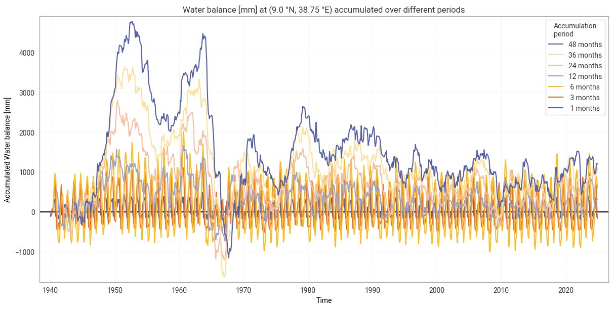
Fig. 6.1.10 Water balance from ERA5 accumulated over different accumulation periods, for the example site of Addis Ababa, Ethiopia.

4.3 Fit logistic distribution and compute SPEI

While SPI assumes a gamma distribution for total precipitation, this does not hold for water balance. For SPEI, various distributions are used in the literature [Stagge+15]. While [Keune+25] specifies that ERA5–Drought’s SPEI is based on the generalised log-logistic distribution, following [Vicente-Serrano+10], private communication with the authors indicates that a generalised logistic distribution is used instead.

As before, the distribution is fitted to data in the reference window (1991–2020), Here, we use scipy.stats.genlogistic to fit the generalised logistic distribution. This returns three parameters for each calendar month and accumulation period, namely shape (c), location (μ), and scale (β).

The observed (accumulated) water balance values along the entire time series are then compared to the fitted parameters in terms of where they fall on the cumulative distribution function (CDF). From these CDF values, SPEI values for each data point (latitude, longitude, time) are calculated by transforming to a standard normal distribution. The zero-precipitation correction from 3. SPI comparison is not relevant to SPEI.

Note that actually evaluating the CDF – as opposed to queueing it up in dask, as done here – can be slow, especially for a large dataset like global ERA5 precipitation and evaporation. As such, if you are interested in a subset of the data, such as a specific site or period in time, it may be best to subset your data before calculating the CDF rather than afterwards. An example of this is provided below in the comparison with ERA5–Drought SPEI.

Show code cell source

Hide code cell source

# Select data in reference window
data_era5_waterbalance_reference = data_era5_waterbalance.sel(**reference_window)

# Fit generalised logistic distribution
spei_parameters = fit_monthly_spei(data_era5_waterbalance_reference)

# Compute CDF time series
cdf = compute_cdf_spei(data_era5_waterbalance, spei_parameters)

# Calculate SPI from adjusted CDF
spei_reproduced = cdf_to_spei(cdf)

# Display result
spei_reproduced

Show code cell output

Hide code cell output

<xarray.Dataset> Size: 59GB
Dimensions:  (time: 1020, lat: 721, lon: 1440)
Coordinates:
    number   int64 8B 0
  * time     (time) datetime64[ns] 8kB 1940-01-01T06:00:00 ... 2024-12-01T06:...
  * lat      (lat) float64 6kB 90.0 89.75 89.5 89.25 ... -89.5 -89.75 -90.0
    expver   (time) <U4 16kB dask.array<chunksize=(1020,), meta=np.ndarray>
  * lon      (lon) float64 12kB -180.0 -179.8 -179.5 ... 179.2 179.5 179.8
    month    (time) int64 8kB dask.array<chunksize=(1020,), meta=np.ndarray>
Data variables:
    SPEI1    (time, lat, lon) float64 8GB dask.array<chunksize=(1020, 103, 360), meta=np.ndarray>
    SPEI3    (time, lat, lon) float64 8GB dask.array<chunksize=(1020, 103, 360), meta=np.ndarray>
    SPEI6    (time, lat, lon) float64 8GB dask.array<chunksize=(1020, 103, 360), meta=np.ndarray>
    SPEI12   (time, lat, lon) float64 8GB dask.array<chunksize=(1020, 103, 360), meta=np.ndarray>
    SPEI24   (time, lat, lon) float64 8GB dask.array<chunksize=(1020, 103, 360), meta=np.ndarray>
    SPEI36   (time, lat, lon) float64 8GB dask.array<chunksize=(1020, 103, 360), meta=np.ndarray>
    SPEI48   (time, lat, lon) float64 8GB dask.array<chunksize=(1020, 103, 360), meta=np.ndarray>

xarray.Dataset

• Dimensions:
  • time: 1020
  • lat: 721
  • lon: 1440
• Coordinates: (6)
  • number
    ()
    int64
    0

    long_name :

    ensemble member numerical id

    units :

    1

    standard_name :

    realization

    array(0)

  • time
    (time)
    datetime64[ns]
    1940-01-01T06:00:00 ... 2024-12-...

    long_name :

    time

    standard_name :

    time

    array(['1940-01-01T06:00:00.000000000', '1940-02-01T06:00:00.000000000',
           '1940-03-01T06:00:00.000000000', ..., '2024-10-01T06:00:00.000000000',
           '2024-11-01T06:00:00.000000000', '2024-12-01T06:00:00.000000000'],
          shape=(1020,), dtype='datetime64[ns]')

  • lat
    (lat)
    float64
    90.0 89.75 89.5 ... -89.75 -90.0

    units :

    degrees_north

    standard_name :

    latitude

    long_name :

    latitude

    stored_direction :

    decreasing

    array([ 90.  ,  89.75,  89.5 , ..., -89.5 , -89.75, -90.  ], shape=(721,))

  • expver
    (time)
    <U4
    dask.array<chunksize=(1020,), meta=np.ndarray>

    Array Chunk Bytes 15.94 kiB 15.94 kiB Shape (1020,) (1020,) Dask graph 1 chunks in 1 graph layer Data type

  • lon
    (lon)
    float64
    -180.0 -179.8 ... 179.5 179.8

    array([-180.  , -179.75, -179.5 , ...,  179.25,  179.5 ,  179.75],
          shape=(1440,))

  • month
    (time)
    int64
    dask.array<chunksize=(1020,), meta=np.ndarray>

    long_name :

    time

    standard_name :

    time

    Array Chunk Bytes 7.97 kiB 7.97 kiB Shape (1020,) (1020,) Dask graph 1 chunks in 1 graph layer Data type int64 numpy.ndarray

• Data variables: (7)
  • SPEI1
    (time, lat, lon)
    float64
    dask.array<chunksize=(1020, 103, 360), meta=np.ndarray>

    Array Chunk Bytes 7.89 GiB 288.56 MiB Shape (1020, 721, 1440) (1020, 103, 360) Dask graph 28 chunks in 119 graph layers Data type float64 numpy.ndarray

  • SPEI3
    (time, lat, lon)
    float64
    dask.array<chunksize=(1020, 103, 360), meta=np.ndarray>

    Array Chunk Bytes 7.89 GiB 288.56 MiB Shape (1020, 721, 1440) (1020, 103, 360) Dask graph 28 chunks in 128 graph layers Data type float64 numpy.ndarray

  • SPEI6
    (time, lat, lon)
    float64
    dask.array<chunksize=(1020, 103, 360), meta=np.ndarray>

    Array Chunk Bytes 7.89 GiB 288.56 MiB Shape (1020, 721, 1440) (1020, 103, 360) Dask graph 28 chunks in 128 graph layers Data type float64 numpy.ndarray

  • SPEI12
    (time, lat, lon)
    float64
    dask.array<chunksize=(1020, 103, 360), meta=np.ndarray>

    Array Chunk Bytes 7.89 GiB 288.56 MiB Shape (1020, 721, 1440) (1020, 103, 360) Dask graph 28 chunks in 128 graph layers Data type float64 numpy.ndarray

  • SPEI24
    (time, lat, lon)
    float64
    dask.array<chunksize=(1020, 103, 360), meta=np.ndarray>

    Array Chunk Bytes 7.89 GiB 288.56 MiB Shape (1020, 721, 1440) (1020, 103, 360) Dask graph 28 chunks in 128 graph layers Data type float64 numpy.ndarray

  • SPEI36
    (time, lat, lon)
    float64
    dask.array<chunksize=(1020, 103, 360), meta=np.ndarray>

    Array Chunk Bytes 7.89 GiB 288.56 MiB Shape (1020, 721, 1440) (1020, 103, 360) Dask graph 28 chunks in 128 graph layers Data type float64 numpy.ndarray

  • SPEI48
    (time, lat, lon)
    float64
    dask.array<chunksize=(1020, 103, 360), meta=np.ndarray>

    Array Chunk Bytes 7.89 GiB 288.56 MiB Shape (1020, 721, 1440) (1020, 103, 360) Dask graph 28 chunks in 128 graph layers Data type float64 numpy.ndarray

• Indexes: (3)
  • time
    PandasIndex

    PandasIndex(DatetimeIndex(['1940-01-01 06:00:00', '1940-02-01 06:00:00',
                   '1940-03-01 06:00:00', '1940-04-01 06:00:00',
                   '1940-05-01 06:00:00', '1940-06-01 06:00:00',
                   '1940-07-01 06:00:00', '1940-08-01 06:00:00',
                   '1940-09-01 06:00:00', '1940-10-01 06:00:00',
                   ...
                   '2024-03-01 06:00:00', '2024-04-01 06:00:00',
                   '2024-05-01 06:00:00', '2024-06-01 06:00:00',
                   '2024-07-01 06:00:00', '2024-08-01 06:00:00',
                   '2024-09-01 06:00:00', '2024-10-01 06:00:00',
                   '2024-11-01 06:00:00', '2024-12-01 06:00:00'],
                  dtype='datetime64[ns]', name='time', length=1020, freq=None))

  • lat
    PandasIndex

    PandasIndex(Index([  90.0,  89.75,   89.5,  89.25,   89.0,  88.75,   88.5,  88.25,   88.0,
            87.75,
           ...
           -87.75,  -88.0, -88.25,  -88.5, -88.75,  -89.0, -89.25,  -89.5, -89.75,
            -90.0],
          dtype='float64', name='lat', length=721))

  • lon
    PandasIndex

    PandasIndex(Index([ -180.0, -179.75,  -179.5, -179.25,  -179.0, -178.75,  -178.5, -178.25,
            -178.0, -177.75,
           ...
             177.5,  177.75,   178.0,  178.25,   178.5,  178.75,   179.0,  179.25,
             179.5,  179.75],
          dtype='float64', name='lon', length=1440))

• Attributes: (0)

4.4 SPEI comparison: Time series in example site

Having reproduced SPEI from ERA5 precipitation and potential evaporation data following the ERA5–Drought methodology, we can now compare the results to assess the reproducibility of ERA5–Drought. We first compare the datasets over time at the example site defined in 2. General setup.

As before, because the global calculation set up in the previous subsections can take a long time to execute, here we sub-select the downloaded ERA5 data and calculate SPEI for the example site only. For convenience, the full SPEI pipeline is wrapped into a single calculate_spei_from_era5 function, as defined in 1. Code setup.

Show code cell source

Hide code cell source

# Select only desired site
data_era5_waterbalance_site = data_era5_waterbalance_preprocessed.sel(**example_site)

# Calculate SPI
spei_reproduced_site = calculate_spei_from_era5(data_era5_waterbalance_site, reference_window=reference_window)

# Persist in memory to speed up analysis – this step may take a few minutes
spei_reproduced_site = spei_reproduced_site.persist()

# Display result
spei_reproduced_site

Show code cell output

Hide code cell output

<xarray.Dataset> Size: 90kB
Dimensions:  (time: 1020)
Coordinates:
    number   int64 8B 0
  * time     (time) datetime64[ns] 8kB 1940-01-01T06:00:00 ... 2024-12-01T06:...
    lat      float64 8B 9.0
    expver   (time) <U4 16kB dask.array<chunksize=(1020,), meta=np.ndarray>
    lon      float64 8B 38.75
    month    (time) int64 8kB dask.array<chunksize=(1020,), meta=np.ndarray>
Data variables:
    SPEI1    (time) float64 8kB dask.array<chunksize=(1020,), meta=np.ndarray>
    SPEI3    (time) float64 8kB dask.array<chunksize=(1020,), meta=np.ndarray>
    SPEI6    (time) float64 8kB dask.array<chunksize=(1020,), meta=np.ndarray>
    SPEI12   (time) float64 8kB dask.array<chunksize=(1020,), meta=np.ndarray>
    SPEI24   (time) float64 8kB dask.array<chunksize=(1020,), meta=np.ndarray>
    SPEI36   (time) float64 8kB dask.array<chunksize=(1020,), meta=np.ndarray>
    SPEI48   (time) float64 8kB dask.array<chunksize=(1020,), meta=np.ndarray>

xarray.Dataset

• Dimensions:
  • time: 1020
• Coordinates: (6)
  • number
    ()
    int64
    0

    long_name :

    ensemble member numerical id

    units :

    1

    standard_name :

    realization

    array(0)

  • time
    (time)
    datetime64[ns]
    1940-01-01T06:00:00 ... 2024-12-...

    long_name :

    time

    standard_name :

    time

    array(['1940-01-01T06:00:00.000000000', '1940-02-01T06:00:00.000000000',
           '1940-03-01T06:00:00.000000000', ..., '2024-10-01T06:00:00.000000000',
           '2024-11-01T06:00:00.000000000', '2024-12-01T06:00:00.000000000'],
          shape=(1020,), dtype='datetime64[ns]')

  • lat
    ()
    float64
    9.0

    units :

    degrees_north

    standard_name :

    latitude

    long_name :

    latitude

    stored_direction :

    decreasing

    array(9.)

  • expver
    (time)
    <U4
    dask.array<chunksize=(1020,), meta=np.ndarray>

    Array Chunk Bytes 15.94 kiB 15.94 kiB Shape (1020,) (1020,) Dask graph 1 chunks in 1 graph layer Data type

  • lon
    ()
    float64
    38.75

    array(38.75)

  • month
    (time)
    int64
    dask.array<chunksize=(1020,), meta=np.ndarray>

    long_name :

    time

    standard_name :

    time

    Array Chunk Bytes 7.97 kiB 7.97 kiB Shape (1020,) (1020,) Dask graph 1 chunks in 1 graph layer Data type int64 numpy.ndarray

• Data variables: (7)
  • SPEI1
    (time)
    float64
    dask.array<chunksize=(1020,), meta=np.ndarray>

    Array Chunk Bytes 7.97 kiB 7.97 kiB Shape (1020,) (1020,) Dask graph 1 chunks in 1 graph layer Data type float64 numpy.ndarray

  • SPEI3
    (time)
    float64
    dask.array<chunksize=(1020,), meta=np.ndarray>

    Array Chunk Bytes 7.97 kiB 7.97 kiB Shape (1020,) (1020,) Dask graph 1 chunks in 1 graph layer Data type float64 numpy.ndarray

  • SPEI6
    (time)
    float64
    dask.array<chunksize=(1020,), meta=np.ndarray>

    Array Chunk Bytes 7.97 kiB 7.97 kiB Shape (1020,) (1020,) Dask graph 1 chunks in 1 graph layer Data type float64 numpy.ndarray

  • SPEI12
    (time)
    float64
    dask.array<chunksize=(1020,), meta=np.ndarray>

    Array Chunk Bytes 7.97 kiB 7.97 kiB Shape (1020,) (1020,) Dask graph 1 chunks in 1 graph layer Data type float64 numpy.ndarray

  • SPEI24
    (time)
    float64
    dask.array<chunksize=(1020,), meta=np.ndarray>

    Array Chunk Bytes 7.97 kiB 7.97 kiB Shape (1020,) (1020,) Dask graph 1 chunks in 1 graph layer Data type float64 numpy.ndarray

  • SPEI36
    (time)
    float64
    dask.array<chunksize=(1020,), meta=np.ndarray>

    Array Chunk Bytes 7.97 kiB 7.97 kiB Shape (1020,) (1020,) Dask graph 1 chunks in 1 graph layer Data type float64 numpy.ndarray

  • SPEI48
    (time)
    float64
    dask.array<chunksize=(1020,), meta=np.ndarray>

    Array Chunk Bytes 7.97 kiB 7.97 kiB Shape (1020,) (1020,) Dask graph 1 chunks in 1 graph layer Data type float64 numpy.ndarray

• Indexes: (1)
  • time
    PandasIndex

    PandasIndex(DatetimeIndex(['1940-01-01 06:00:00', '1940-02-01 06:00:00',
                   '1940-03-01 06:00:00', '1940-04-01 06:00:00',
                   '1940-05-01 06:00:00', '1940-06-01 06:00:00',
                   '1940-07-01 06:00:00', '1940-08-01 06:00:00',
                   '1940-09-01 06:00:00', '1940-10-01 06:00:00',
                   ...
                   '2024-03-01 06:00:00', '2024-04-01 06:00:00',
                   '2024-05-01 06:00:00', '2024-06-01 06:00:00',
                   '2024-07-01 06:00:00', '2024-08-01 06:00:00',
                   '2024-09-01 06:00:00', '2024-10-01 06:00:00',
                   '2024-11-01 06:00:00', '2024-12-01 06:00:00'],
                  dtype='datetime64[ns]', name='time', length=1020, freq=None))

• Attributes: (0)

Next, we download the corresponding data from ERA5–Drought. Because of size limits on the CDS, the time series must be downloaded in parts:

Show code cell source

Hide code cell source

# Main request, based on template and example site
request_era5drought_spei = {
    "variable": ["standardised_precipitation_evapotranspiration_index"],
} | request_era5drought_index | request_site

# Split into batches of up to 20 years each
subrequests_era5drought_spei = batch_requests(request_era5drought_spei, n=20)

# Download data and load into xarray
spei_era5drought_site = ekd.from_source("cds", ID_ERA5_DROUGHT, *subrequests_era5drought_spei)
spei_era5drought_site = spei_era5drought_site.to_xarray(compat="equals", join="outer")
spei_era5drought_site = spei_era5drought_site.chunk({"time": -1})  # Full time series in one chunk

# Select only desired site (remove margins)
spei_era5drought_site = spei_era5drought_site.sel(**example_site)

# Persist in memory to speed up analysis – this step may take a few minutes
spei_era5drought_site = spei_era5drought_site.persist()

# Display result
spei_era5drought_site

Show code cell output

Hide code cell output

<xarray.Dataset> Size: 65kB
Dimensions:  (time: 1020)
Coordinates:
  * time     (time) datetime64[ns] 8kB 1940-01-01T06:00:00 ... 2024-12-01T06:...
    lat      float64 8B 9.0
    lon      float64 8B 38.75
Data variables:
    SPEI12   (time) float64 8kB dask.array<chunksize=(1020,), meta=np.ndarray>
    SPEI1    (time) float64 8kB dask.array<chunksize=(1020,), meta=np.ndarray>
    SPEI24   (time) float64 8kB dask.array<chunksize=(1020,), meta=np.ndarray>
    SPEI36   (time) float64 8kB dask.array<chunksize=(1020,), meta=np.ndarray>
    SPEI3    (time) float64 8kB dask.array<chunksize=(1020,), meta=np.ndarray>
    SPEI48   (time) float64 8kB dask.array<chunksize=(1020,), meta=np.ndarray>
    SPEI6    (time) float64 8kB dask.array<chunksize=(1020,), meta=np.ndarray>
Attributes: (12/17)
    title:                   SPEI12
    description:             Drought Index: Standardized Drought Index calcul...
    Conventions:             CF-1.8
    history:                 Created 13/08/2024 14:50:12 using DRYFALL.
    institution:             European Centre for Medium-Range Weather Forecasts
    source:                  DRYFALL v1.0
    ...                      ...
    climate_start_date:      1991-01-01
    climate_end_date:        2020-12-31
    frequency:               Monthly
    contact_person:          support@ecmwf.int
    ref_publication:         Keune, J., Di Giuseppe, F., Barnard, C., Damasio...
    cds_data_catalogue_url:  https://cds.climate.copernicus.eu/datasets/deriv...

xarray.Dataset

• Dimensions:
  • time: 1020
• Coordinates: (3)
  • time
    (time)
    datetime64[ns]
    1940-01-01T06:00:00 ... 2024-12-...

    standard_name :

    time

    array(['1940-01-01T06:00:00.000000000', '1940-02-01T06:00:00.000000000',
           '1940-03-01T06:00:00.000000000', ..., '2024-10-01T06:00:00.000000000',
           '2024-11-01T06:00:00.000000000', '2024-12-01T06:00:00.000000000'],
          shape=(1020,), dtype='datetime64[ns]')

  • lat
    ()
    float64
    9.0

    units :

    degrees_north

    long_name :

    degrees_north

    array(9.)

  • lon
    ()
    float64
    38.75

    units :

    degrees_east

    long_name :

    degrees_east

    array(38.75)

• Data variables: (7)
  • SPEI12
    (time)
    float64
    dask.array<chunksize=(1020,), meta=np.ndarray>

    long_name :

    Standardized Drought Index (SPEI12)

    Array Chunk Bytes 7.97 kiB 7.97 kiB Shape (1020,) (1020,) Dask graph 1 chunks in 1 graph layer Data type float64 numpy.ndarray

  • SPEI1
    (time)
    float64
    dask.array<chunksize=(1020,), meta=np.ndarray>

    long_name :

    Standardized Drought Index (SPEI1)

    Array Chunk Bytes 7.97 kiB 7.97 kiB Shape (1020,) (1020,) Dask graph 1 chunks in 1 graph layer Data type float64 numpy.ndarray

  • SPEI24
    (time)
    float64
    dask.array<chunksize=(1020,), meta=np.ndarray>

    long_name :

    Standardized Drought Index (SPEI24)

    Array Chunk Bytes 7.97 kiB 7.97 kiB Shape (1020,) (1020,) Dask graph 1 chunks in 1 graph layer Data type float64 numpy.ndarray

  • SPEI36
    (time)
    float64
    dask.array<chunksize=(1020,), meta=np.ndarray>

    long_name :

    Standardized Drought Index (SPEI36)

    Array Chunk Bytes 7.97 kiB 7.97 kiB Shape (1020,) (1020,) Dask graph 1 chunks in 1 graph layer Data type float64 numpy.ndarray

  • SPEI3
    (time)
    float64
    dask.array<chunksize=(1020,), meta=np.ndarray>

    long_name :

    Standardized Drought Index (SPEI3)

    Array Chunk Bytes 7.97 kiB 7.97 kiB Shape (1020,) (1020,) Dask graph 1 chunks in 1 graph layer Data type float64 numpy.ndarray

  • SPEI48
    (time)
    float64
    dask.array<chunksize=(1020,), meta=np.ndarray>

    long_name :

    Standardized Drought Index (SPEI48)

    Array Chunk Bytes 7.97 kiB 7.97 kiB Shape (1020,) (1020,) Dask graph 1 chunks in 1 graph layer Data type float64 numpy.ndarray

  • SPEI6
    (time)
    float64
    dask.array<chunksize=(1020,), meta=np.ndarray>

    long_name :

    Standardized Drought Index (SPEI6)

    Array Chunk Bytes 7.97 kiB 7.97 kiB Shape (1020,) (1020,) Dask graph 1 chunks in 1 graph layer Data type float64 numpy.ndarray

• Indexes: (1)
  • time
    PandasIndex

    PandasIndex(DatetimeIndex(['1940-01-01 06:00:00', '1940-02-01 06:00:00',
                   '1940-03-01 06:00:00', '1940-04-01 06:00:00',
                   '1940-05-01 06:00:00', '1940-06-01 06:00:00',
                   '1940-07-01 06:00:00', '1940-08-01 06:00:00',
                   '1940-09-01 06:00:00', '1940-10-01 06:00:00',
                   ...
                   '2024-03-01 06:00:00', '2024-04-01 06:00:00',
                   '2024-05-01 06:00:00', '2024-06-01 06:00:00',
                   '2024-07-01 06:00:00', '2024-08-01 06:00:00',
                   '2024-09-01 06:00:00', '2024-10-01 06:00:00',
                   '2024-11-01 06:00:00', '2024-12-01 06:00:00'],
                  dtype='datetime64[ns]', name='time', length=1020, freq='MS'))

• Attributes: (17)

  title :

  SPEI12

  description :

  Drought Index: Standardized Drought Index calculated according to the WMO guidelines (see https://library.wmo.int/doc_num.php?explnum_id=7768).

  Conventions :

  CF-1.8

  history :

  Created 13/08/2024 14:50:12 using DRYFALL.

  institution :

  European Centre for Medium-Range Weather Forecasts

  source :

  DRYFALL v1.0

  license :

  Creative Commons Attribution v4

  citation_statement :

  Drought indicators derived from ERA5 reanalysis

  data_srs :

  EPSG:4326

  extent :

  -180,-90,180,90

  resolution :

  0.25x0.25

  climate_start_date :

  1991-01-01

  climate_end_date :

  2020-12-31

  frequency :

  Monthly

  contact_person :

  support@ecmwf.int

  ref_publication :

  Keune, J., Di Giuseppe, F., Barnard, C., Damasio da Costa, E., and Wetterhall, F. (2025): ERA5–Drought: Global drought indices based on ECMWF reanalysis, Scientific Data 12, 616. https://doi.org/10.1038/s41597-025-04896-y

  cds_data_catalogue_url :

  https://cds.climate.copernicus.eu/datasets/derived-drought-historical-monthly

Again, we examine the per-point difference in SPEI between ERA5–Drought and the reproduction for each calendar month and each accumulation period. We calculate the median difference MΔ and median absolute difference M|Δ|, as well as the percentage of match-ups where |Δ| ≥ 0.10:

Show code cell source

Hide code cell source

# Calculate SPEI median differences
spei_difference_site = comparison_monthly_statistics(spei_era5drought_site, spei_reproduced_site)

# Display with style
display_monthly_statistics(spei_difference_site)

Reproduced – ERA5–Drought

	SPEI-1			SPEI-3			SPEI-6			SPEI-12			SPEI-24			SPEI-36			SPEI-48
	MΔ	M|Δ|	|Δ| ≥ 0.10	MΔ	M|Δ|	|Δ| ≥ 0.10	MΔ	M|Δ|	|Δ| ≥ 0.10	MΔ	M|Δ|	|Δ| ≥ 0.10	MΔ	M|Δ|	|Δ| ≥ 0.10	MΔ	M|Δ|	|Δ| ≥ 0.10	MΔ	M|Δ|	|Δ| ≥ 0.10
January	0.0000	0.0000	0.0000	0.0000	0.0000	0.0000	-0.0000	0.0000	0.0000	-0.0000	0.0000	0.0000	-0.0000	0.0000	0.0000	0.0000	0.0000	0.0000	0.0000	0.0000	0.0000
February	0.0135	0.0162	0.0000	0.0068	0.0106	0.0000	-0.0003	0.0240	0.0000	0.0065	0.0133	1.1765	-0.0429	0.0439	3.5294	-0.0131	0.0315	0.0000	0.0180	0.0349	11.7647
March	0.0041	0.0203	0.0000	0.0223	0.0319	0.0000	0.0021	0.0175	0.0000	0.0070	0.0287	4.7059	-0.0489	0.0497	3.5294	-0.0083	0.0356	2.3529	0.0120	0.0334	3.5294
April	-0.0153	0.0153	0.0000	0.0042	0.0226	0.0000	-0.0026	0.0252	1.1765	-0.0020	0.0276	3.5294	-0.0102	0.0326	3.5294	-0.0699	0.0699	18.8235	0.0248	0.0285	11.7647
May	-0.0380	0.0380	0.0000	-0.0275	0.0312	2.3529	-0.0248	0.0255	0.0000	-0.0367	0.0411	2.3529	0.0019	0.0326	5.8824	-0.0558	0.0558	0.0000	-0.0013	0.0102	4.7059
June	-0.0249	0.0280	0.0000	-0.0396	0.0396	0.0000	-0.0255	0.0264	0.0000	-0.0250	0.0250	0.0000	0.0137	0.0248	2.3529	-0.1022	0.1022	49.4118	0.0085	0.0316	20.0000
July	-0.0334	0.0354	2.3529	-0.0472	0.0487	2.3529	-0.0346	0.0355	0.0000	-0.0278	0.0278	0.0000	-0.0094	0.0547	23.5294	-0.1233	0.1233	49.4118	0.0181	0.0462	23.5294
August	-0.0228	0.0288	1.1765	-0.0343	0.0931	48.2353	-0.0384	0.0387	4.7059	-0.0465	0.0466	1.1765	-0.0015	0.0403	15.2941	-0.1525	0.1525	57.6471	0.0065	0.0563	21.1765
September	-0.0050	0.0238	0.0000	-0.0275	0.0318	0.0000	-0.0498	0.0498	0.0000	-0.0347	0.0369	3.5294	0.0044	0.0358	16.4706	-0.1424	0.1424	52.9412	-0.0326	0.0381	1.1765
October	0.0112	0.0161	0.0000	0.0019	0.0426	1.1765	-0.0469	0.0477	0.0000	-0.0347	0.0348	0.0000	-0.0006	0.0491	21.1765	-0.1220	0.1220	50.5882	-0.0296	0.0349	1.1765
November	0.0190	0.0198	0.0000	0.0080	0.0228	0.0000	-0.0115	0.0460	4.7059	-0.0255	0.0264	1.1765	0.0065	0.0362	11.7647	-0.1140	0.1140	52.9412	-0.0238	0.0396	2.3529
December	0.0118	0.0159	0.0000	0.0307	0.0307	0.0000	-0.0107	0.0475	14.1176	-0.0217	0.0236	4.7059	0.0074	0.0444	21.1765	-0.1287	0.1287	55.2941	-0.0314	0.0363	2.3529

At first glance, agreement in SPEI is considerably worse than in SPI. This shows in non-zero median and median absolute differences for most calendar month–accumulation period pairs, as well as larger percentages of match-ups that exceed the threshold of 0.10 difference. These patterns are visible in the time series comparison (Figure 6.1.11) in the form of noticeable scatter about the 0-line, in addition to a few spikes like those seen in Figure 6.1.2.

However, agreement is still good in general, and the discrepancies seen above rarely lead to differences in classification (Figure 6.1.12). This is particularly important for SPEI-36, where differences in 1950–1970 are large but do not change the resulting classification.

The most likely cause for the increased difference is the choice of statistical distribution. As noted above, it is not entirely clear which distribution underpins ERA5–Drought’s SPEI values, and the scipy.stats.genlogistic implementation used in this notebook may not be the same one. For example, Wikipedia lists four different generalised logistic distributions. If the distribution used in ERA5–Drought is not equal to, but similar to, the implementation used in this notebook, that may well result in consistent, small differences in the exact values but good agreement overall – as seen in this analysis.

Show code cell source

Hide code cell source

# Plot time series comparison (absolute values and differences)
plot_time_series_comparison_spei(spei_era5drought_site, spei_reproduced_site, title_suffix=f" at {label_site}",
                                 glue_label="indicator_derived-drought-historical-monthly_consistency_q01_fig-spei-timeseries")

Show code cell source

Hide code cell source

# Plot confusion matrix comparison
# e.g. are all "extremely dry" data in ERA5–Drought also "extremely dry" in the reproduction?
plot_confusion_matrices_spei(spei_era5drought_site, spei_reproduced_site, title_suffix=f" at {label_site}",
                             glue_label="indicator_derived-drought-historical-monthly_consistency_q01_fig-spei-confusion")

Time series

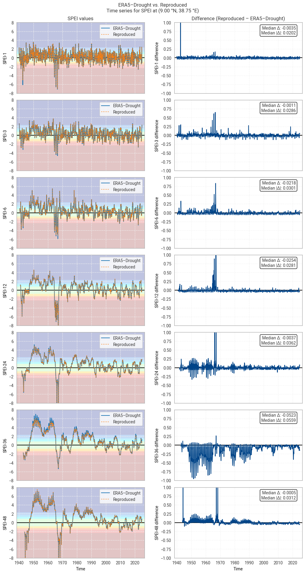
Fig. 6.1.11 SPEI time series downloaded from ERA5–Drought and reproduced from ERA5 precipitation data (left) and the difference between the two (right), for the example site of Addis Ababa, Ethiopia. Colours in the left-hand column correspond to SPEI categories (e.g. “extremely dry”) in [Keune+25].

Confusion matrix

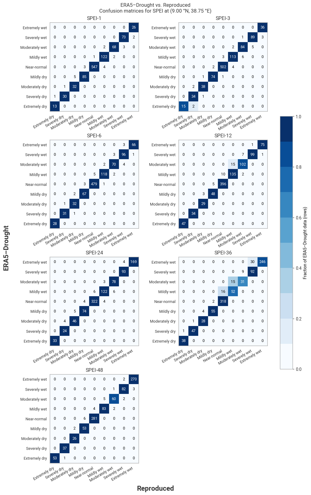
Fig. 6.1.12 Confusion matrices for SPEI categories from ERA5–Drought vs. reproduced from ERA5, for the example site of Addis Ababa, Ethiopia, in 1940–2024.

4.5 SPEI comparison: Regional snapshot

Next, we investigate spatial patterns in SPEI and the difference therein across a wider region around the example site. This region is defined in 2. General setup. In this example, we look at part of the Horn of Africa using a box of 12° in all directions around Addis Ababa, Ethiopia. To reduce computing requirements, the comparison is performed for one year only, here 2024, again defined in 2. General setup.

As in the time series comparison, we subselect the desired data from ERA5 and calculate the corresponding SPEI and download SPEI from ERA5–Drought for the desired region and time span:

Show code cell source

Hide code cell source

# Select only desired site
data_era5_waterbalance_region = data_era5_waterbalance_preprocessed.sel(**example_region)

# Window in which to evaluate SPI
evaluation_window = {"time": slice(f"{year_snapshot}-01-01", f"{year_snapshot}-12-01")}  #  Slice (2024-01-01, 2024-12-01)

# Calculate SPI
spei_reproduced_region = calculate_spei_from_era5(data_era5_waterbalance_region, reference_window=reference_window,
                                                  evaluation_window=evaluation_window)

# Persist in memory to speed up analysis – this step may take a few minutes
spei_reproduced_region = spei_reproduced_region.persist()

# Display result
spei_reproduced_region

Show code cell output

Hide code cell output

<xarray.Dataset> Size: 6MB
Dimensions:  (time: 12, lat: 97, lon: 97)
Coordinates:
    number   int64 8B 0
  * time     (time) datetime64[ns] 96B 2024-01-01T06:00:00 ... 2024-12-01T06:...
  * lat      (lat) float64 776B 21.0 20.75 20.5 20.25 ... -2.25 -2.5 -2.75 -3.0
    expver   (time) <U4 192B dask.array<chunksize=(12,), meta=np.ndarray>
  * lon      (lon) float64 776B 26.75 27.0 27.25 27.5 ... 50.0 50.25 50.5 50.75
    month    (time) int64 96B dask.array<chunksize=(12,), meta=np.ndarray>
Data variables:
    SPEI1    (time, lat, lon) float64 903kB dask.array<chunksize=(12, 33, 97), meta=np.ndarray>
    SPEI3    (time, lat, lon) float64 903kB dask.array<chunksize=(12, 33, 97), meta=np.ndarray>
    SPEI6    (time, lat, lon) float64 903kB dask.array<chunksize=(12, 33, 97), meta=np.ndarray>
    SPEI12   (time, lat, lon) float64 903kB dask.array<chunksize=(12, 33, 97), meta=np.ndarray>
    SPEI24   (time, lat, lon) float64 903kB dask.array<chunksize=(12, 33, 97), meta=np.ndarray>
    SPEI36   (time, lat, lon) float64 903kB dask.array<chunksize=(12, 33, 97), meta=np.ndarray>
    SPEI48   (time, lat, lon) float64 903kB dask.array<chunksize=(12, 33, 97), meta=np.ndarray>

xarray.Dataset

• Dimensions:
  • time: 12
  • lat: 97
  • lon: 97
• Coordinates: (6)
  • number
    ()
    int64
    0

    long_name :

    ensemble member numerical id

    units :

    1

    standard_name :

    realization

    array(0)

  • time
    (time)
    datetime64[ns]
    2024-01-01T06:00:00 ... 2024-12-...

    long_name :

    time

    standard_name :

    time

    array(['2024-01-01T06:00:00.000000000', '2024-02-01T06:00:00.000000000',
           '2024-03-01T06:00:00.000000000', '2024-04-01T06:00:00.000000000',
           '2024-05-01T06:00:00.000000000', '2024-06-01T06:00:00.000000000',
           '2024-07-01T06:00:00.000000000', '2024-08-01T06:00:00.000000000',
           '2024-09-01T06:00:00.000000000', '2024-10-01T06:00:00.000000000',
           '2024-11-01T06:00:00.000000000', '2024-12-01T06:00:00.000000000'],
          dtype='datetime64[ns]')

  • lat
    (lat)
    float64
    21.0 20.75 20.5 ... -2.5 -2.75 -3.0

    units :

    degrees_north

    standard_name :

    latitude

    long_name :

    latitude

    stored_direction :

    decreasing

    array([21.  , 20.75, 20.5 , 20.25, 20.  , 19.75, 19.5 , 19.25, 19.  , 18.75,
           18.5 , 18.25, 18.  , 17.75, 17.5 , 17.25, 17.  , 16.75, 16.5 , 16.25,
           16.  , 15.75, 15.5 , 15.25, 15.  , 14.75, 14.5 , 14.25, 14.  , 13.75,
           13.5 , 13.25, 13.  , 12.75, 12.5 , 12.25, 12.  , 11.75, 11.5 , 11.25,
           11.  , 10.75, 10.5 , 10.25, 10.  ,  9.75,  9.5 ,  9.25,  9.  ,  8.75,
            8.5 ,  8.25,  8.  ,  7.75,  7.5 ,  7.25,  7.  ,  6.75,  6.5 ,  6.25,
            6.  ,  5.75,  5.5 ,  5.25,  5.  ,  4.75,  4.5 ,  4.25,  4.  ,  3.75,
            3.5 ,  3.25,  3.  ,  2.75,  2.5 ,  2.25,  2.  ,  1.75,  1.5 ,  1.25,
            1.  ,  0.75,  0.5 ,  0.25,  0.  , -0.25, -0.5 , -0.75, -1.  , -1.25,
           -1.5 , -1.75, -2.  , -2.25, -2.5 , -2.75, -3.  ])

  • expver
    (time)
    <U4
    dask.array<chunksize=(12,), meta=np.ndarray>

    Array Chunk Bytes 192 B 192 B Shape (12,) (12,) Dask graph 1 chunks in 1 graph layer Data type

  • lon
    (lon)
    float64
    26.75 27.0 27.25 ... 50.5 50.75

    array([26.75, 27.  , 27.25, 27.5 , 27.75, 28.  , 28.25, 28.5 , 28.75, 29.  ,
           29.25, 29.5 , 29.75, 30.  , 30.25, 30.5 , 30.75, 31.  , 31.25, 31.5 ,
           31.75, 32.  , 32.25, 32.5 , 32.75, 33.  , 33.25, 33.5 , 33.75, 34.  ,
           34.25, 34.5 , 34.75, 35.  , 35.25, 35.5 , 35.75, 36.  , 36.25, 36.5 ,
           36.75, 37.  , 37.25, 37.5 , 37.75, 38.  , 38.25, 38.5 , 38.75, 39.  ,
           39.25, 39.5 , 39.75, 40.  , 40.25, 40.5 , 40.75, 41.  , 41.25, 41.5 ,
           41.75, 42.  , 42.25, 42.5 , 42.75, 43.  , 43.25, 43.5 , 43.75, 44.  ,
           44.25, 44.5 , 44.75, 45.  , 45.25, 45.5 , 45.75, 46.  , 46.25, 46.5 ,
           46.75, 47.  , 47.25, 47.5 , 47.75, 48.  , 48.25, 48.5 , 48.75, 49.  ,
           49.25, 49.5 , 49.75, 50.  , 50.25, 50.5 , 50.75])

  • month
    (time)
    int64
    dask.array<chunksize=(12,), meta=np.ndarray>

    long_name :

    time

    standard_name :

    time

    Array Chunk Bytes 96 B 96 B Shape (12,) (12,) Dask graph 1 chunks in 1 graph layer Data type int64 numpy.ndarray

• Data variables: (7)
  • SPEI1
    (time, lat, lon)
    float64
    dask.array<chunksize=(12, 33, 97), meta=np.ndarray>

    Array Chunk Bytes 882.09 kiB 582.00 kiB Shape (12, 97, 97) (12, 64, 97) Dask graph 2 chunks in 1 graph layer Data type float64 numpy.ndarray

  • SPEI3
    (time, lat, lon)
    float64
    dask.array<chunksize=(12, 33, 97), meta=np.ndarray>

    Array Chunk Bytes 882.09 kiB 582.00 kiB Shape (12, 97, 97) (12, 64, 97) Dask graph 2 chunks in 1 graph layer Data type float64 numpy.ndarray

  • SPEI6
    (time, lat, lon)
    float64
    dask.array<chunksize=(12, 33, 97), meta=np.ndarray>

    Array Chunk Bytes 882.09 kiB 582.00 kiB Shape (12, 97, 97) (12, 64, 97) Dask graph 2 chunks in 1 graph layer Data type float64 numpy.ndarray

  • SPEI12
    (time, lat, lon)
    float64
    dask.array<chunksize=(12, 33, 97), meta=np.ndarray>

    Array Chunk Bytes 882.09 kiB 582.00 kiB Shape (12, 97, 97) (12, 64, 97) Dask graph 2 chunks in 1 graph layer Data type float64 numpy.ndarray

  • SPEI24
    (time, lat, lon)
    float64
    dask.array<chunksize=(12, 33, 97), meta=np.ndarray>

    Array Chunk Bytes 882.09 kiB 582.00 kiB Shape (12, 97, 97) (12, 64, 97) Dask graph 2 chunks in 1 graph layer Data type float64 numpy.ndarray

  • SPEI36
    (time, lat, lon)
    float64
    dask.array<chunksize=(12, 33, 97), meta=np.ndarray>

    Array Chunk Bytes 882.09 kiB 582.00 kiB Shape (12, 97, 97) (12, 64, 97) Dask graph 2 chunks in 1 graph layer Data type float64 numpy.ndarray

  • SPEI48
    (time, lat, lon)
    float64
    dask.array<chunksize=(12, 33, 97), meta=np.ndarray>

    Array Chunk Bytes 882.09 kiB 582.00 kiB Shape (12, 97, 97) (12, 64, 97) Dask graph 2 chunks in 1 graph layer Data type float64 numpy.ndarray

• Indexes: (3)
  • time
    PandasIndex

    PandasIndex(DatetimeIndex(['2024-01-01 06:00:00', '2024-02-01 06:00:00',
                   '2024-03-01 06:00:00', '2024-04-01 06:00:00',
                   '2024-05-01 06:00:00', '2024-06-01 06:00:00',
                   '2024-07-01 06:00:00', '2024-08-01 06:00:00',
                   '2024-09-01 06:00:00', '2024-10-01 06:00:00',
                   '2024-11-01 06:00:00', '2024-12-01 06:00:00'],
                  dtype='datetime64[ns]', name='time', freq=None))

  • lat
    PandasIndex

    PandasIndex(Index([ 21.0, 20.75,  20.5, 20.25,  20.0, 19.75,  19.5, 19.25,  19.0, 18.75,
            18.5, 18.25,  18.0, 17.75,  17.5, 17.25,  17.0, 16.75,  16.5, 16.25,
            16.0, 15.75,  15.5, 15.25,  15.0, 14.75,  14.5, 14.25,  14.0, 13.75,
            13.5, 13.25,  13.0, 12.75,  12.5, 12.25,  12.0, 11.75,  11.5, 11.25,
            11.0, 10.75,  10.5, 10.25,  10.0,  9.75,   9.5,  9.25,   9.0,  8.75,
             8.5,  8.25,   8.0,  7.75,   7.5,  7.25,   7.0,  6.75,   6.5,  6.25,
             6.0,  5.75,   5.5,  5.25,   5.0,  4.75,   4.5,  4.25,   4.0,  3.75,
             3.5,  3.25,   3.0,  2.75,   2.5,  2.25,   2.0,  1.75,   1.5,  1.25,
             1.0,  0.75,   0.5,  0.25,   0.0, -0.25,  -0.5, -0.75,  -1.0, -1.25,
            -1.5, -1.75,  -2.0, -2.25,  -2.5, -2.75,  -3.0],
          dtype='float64', name='lat'))

  • lon
    PandasIndex

    PandasIndex(Index([26.75,  27.0, 27.25,  27.5, 27.75,  28.0, 28.25,  28.5, 28.75,  29.0,
           29.25,  29.5, 29.75,  30.0, 30.25,  30.5, 30.75,  31.0, 31.25,  31.5,
           31.75,  32.0, 32.25,  32.5, 32.75,  33.0, 33.25,  33.5, 33.75,  34.0,
           34.25,  34.5, 34.75,  35.0, 35.25,  35.5, 35.75,  36.0, 36.25,  36.5,
           36.75,  37.0, 37.25,  37.5, 37.75,  38.0, 38.25,  38.5, 38.75,  39.0,
           39.25,  39.5, 39.75,  40.0, 40.25,  40.5, 40.75,  41.0, 41.25,  41.5,
           41.75,  42.0, 42.25,  42.5, 42.75,  43.0, 43.25,  43.5, 43.75,  44.0,
           44.25,  44.5, 44.75,  45.0, 45.25,  45.5, 45.75,  46.0, 46.25,  46.5,
           46.75,  47.0, 47.25,  47.5, 47.75,  48.0, 48.25,  48.5, 48.75,  49.0,
           49.25,  49.5, 49.75,  50.0, 50.25,  50.5, 50.75],
          dtype='float64', name='lon'))

• Attributes: (0)

Show code cell source

Hide code cell source

# Main request, based on template and example region
request_era5drought_spei = {
    "variable": ["standardised_precipitation_evapotranspiration_index"],
} | request_era5drought_index | request_region

# Select only desired year
request_era5drought_spei = request_era5drought_spei | {"year": [f"{year_snapshot}"],}

# Download data and load into xarray
spei_era5drought_region = ekd.from_source("cds", ID_ERA5_DROUGHT, request_era5drought_spei)
spei_era5drought_region = spei_era5drought_region.to_xarray(compat="equals", join="outer")
spei_era5drought_region = spei_era5drought_region.chunk({"time": -1})  # Full time series in one chunk

# Persist in memory to speed up analysis – this step may take a few minutes
spei_era5drought_region = spei_era5drought_region.persist()

# Display result
spei_era5drought_region

Show code cell output

Hide code cell output

<xarray.Dataset> Size: 6MB
Dimensions:  (time: 12, lat: 97, lon: 97)
Coordinates:
  * time     (time) datetime64[ns] 96B 2024-01-01T06:00:00 ... 2024-12-01T06:...
  * lat      (lat) float64 776B 21.0 20.75 20.5 20.25 ... -2.25 -2.5 -2.75 -3.0
  * lon      (lon) float64 776B 26.75 27.0 27.25 27.5 ... 50.0 50.25 50.5 50.75
Data variables:
    SPEI12   (time, lat, lon) float64 903kB dask.array<chunksize=(12, 97, 97), meta=np.ndarray>
    SPEI1    (time, lat, lon) float64 903kB dask.array<chunksize=(12, 97, 97), meta=np.ndarray>
    SPEI24   (time, lat, lon) float64 903kB dask.array<chunksize=(12, 97, 97), meta=np.ndarray>
    SPEI36   (time, lat, lon) float64 903kB dask.array<chunksize=(12, 97, 97), meta=np.ndarray>
    SPEI3    (time, lat, lon) float64 903kB dask.array<chunksize=(12, 97, 97), meta=np.ndarray>
    SPEI48   (time, lat, lon) float64 903kB dask.array<chunksize=(12, 97, 97), meta=np.ndarray>
    SPEI6    (time, lat, lon) float64 903kB dask.array<chunksize=(12, 97, 97), meta=np.ndarray>
Attributes: (12/17)
    title:                   SPEI12
    description:             Drought Index: Standardized Drought Index calcul...
    Conventions:             CF-1.8
    history:                 Created 30/10/2024 07:49:35 using DRYFALL.
    institution:             European Centre for Medium-Range Weather Forecasts
    source:                  DRYFALL v1.0
    ...                      ...
    climate_start_date:      1991-01-01
    climate_end_date:        2020-12-31
    frequency:               Monthly
    contact_person:          support@ecmwf.int
    ref_publication:         Keune, J., Di Giuseppe, F., Barnard, C., Damasio...
    cds_data_catalogue_url:  https://cds.climate.copernicus.eu/datasets/deriv...

xarray.Dataset

• Dimensions:
  • time: 12
  • lat: 97
  • lon: 97
• Coordinates: (3)
  • time
    (time)
    datetime64[ns]
    2024-01-01T06:00:00 ... 2024-12-...

    standard_name :

    time

    array(['2024-01-01T06:00:00.000000000', '2024-02-01T06:00:00.000000000',
           '2024-03-01T06:00:00.000000000', '2024-04-01T06:00:00.000000000',
           '2024-05-01T06:00:00.000000000', '2024-06-01T06:00:00.000000000',
           '2024-07-01T06:00:00.000000000', '2024-08-01T06:00:00.000000000',
           '2024-09-01T06:00:00.000000000', '2024-10-01T06:00:00.000000000',
           '2024-11-01T06:00:00.000000000', '2024-12-01T06:00:00.000000000'],
          dtype='datetime64[ns]')

  • lat
    (lat)
    float64
    21.0 20.75 20.5 ... -2.5 -2.75 -3.0

    units :

    degrees_north

    long_name :

    degrees_north

    array([21.  , 20.75, 20.5 , 20.25, 20.  , 19.75, 19.5 , 19.25, 19.  , 18.75,
           18.5 , 18.25, 18.  , 17.75, 17.5 , 17.25, 17.  , 16.75, 16.5 , 16.25,
           16.  , 15.75, 15.5 , 15.25, 15.  , 14.75, 14.5 , 14.25, 14.  , 13.75,
           13.5 , 13.25, 13.  , 12.75, 12.5 , 12.25, 12.  , 11.75, 11.5 , 11.25,
           11.  , 10.75, 10.5 , 10.25, 10.  ,  9.75,  9.5 ,  9.25,  9.  ,  8.75,
            8.5 ,  8.25,  8.  ,  7.75,  7.5 ,  7.25,  7.  ,  6.75,  6.5 ,  6.25,
            6.  ,  5.75,  5.5 ,  5.25,  5.  ,  4.75,  4.5 ,  4.25,  4.  ,  3.75,
            3.5 ,  3.25,  3.  ,  2.75,  2.5 ,  2.25,  2.  ,  1.75,  1.5 ,  1.25,
            1.  ,  0.75,  0.5 ,  0.25,  0.  , -0.25, -0.5 , -0.75, -1.  , -1.25,
           -1.5 , -1.75, -2.  , -2.25, -2.5 , -2.75, -3.  ])

  • lon
    (lon)
    float64
    26.75 27.0 27.25 ... 50.5 50.75

    units :

    degrees_east

    long_name :

    degrees_east

    array([26.75, 27.  , 27.25, 27.5 , 27.75, 28.  , 28.25, 28.5 , 28.75, 29.  ,
           29.25, 29.5 , 29.75, 30.  , 30.25, 30.5 , 30.75, 31.  , 31.25, 31.5 ,
           31.75, 32.  , 32.25, 32.5 , 32.75, 33.  , 33.25, 33.5 , 33.75, 34.  ,
           34.25, 34.5 , 34.75, 35.  , 35.25, 35.5 , 35.75, 36.  , 36.25, 36.5 ,
           36.75, 37.  , 37.25, 37.5 , 37.75, 38.  , 38.25, 38.5 , 38.75, 39.  ,
           39.25, 39.5 , 39.75, 40.  , 40.25, 40.5 , 40.75, 41.  , 41.25, 41.5 ,
           41.75, 42.  , 42.25, 42.5 , 42.75, 43.  , 43.25, 43.5 , 43.75, 44.  ,
           44.25, 44.5 , 44.75, 45.  , 45.25, 45.5 , 45.75, 46.  , 46.25, 46.5 ,
           46.75, 47.  , 47.25, 47.5 , 47.75, 48.  , 48.25, 48.5 , 48.75, 49.  ,
           49.25, 49.5 , 49.75, 50.  , 50.25, 50.5 , 50.75])

• Data variables: (7)
  • SPEI12
    (time, lat, lon)
    float64
    dask.array<chunksize=(12, 97, 97), meta=np.ndarray>

    long_name :

    Standardized Drought Index (SPEI12)

    Array Chunk Bytes 882.09 kiB 882.09 kiB Shape (12, 97, 97) (12, 97, 97) Dask graph 1 chunks in 1 graph layer Data type float64 numpy.ndarray

  • SPEI1
    (time, lat, lon)
    float64
    dask.array<chunksize=(12, 97, 97), meta=np.ndarray>

    long_name :

    Standardized Drought Index (SPEI1)

    Array Chunk Bytes 882.09 kiB 882.09 kiB Shape (12, 97, 97) (12, 97, 97) Dask graph 1 chunks in 1 graph layer Data type float64 numpy.ndarray

  • SPEI24
    (time, lat, lon)
    float64
    dask.array<chunksize=(12, 97, 97), meta=np.ndarray>

    long_name :

    Standardized Drought Index (SPEI24)

    Array Chunk Bytes 882.09 kiB 882.09 kiB Shape (12, 97, 97) (12, 97, 97) Dask graph 1 chunks in 1 graph layer Data type float64 numpy.ndarray

  • SPEI36
    (time, lat, lon)
    float64
    dask.array<chunksize=(12, 97, 97), meta=np.ndarray>

    long_name :

    Standardized Drought Index (SPEI36)

    Array Chunk Bytes 882.09 kiB 882.09 kiB Shape (12, 97, 97) (12, 97, 97) Dask graph 1 chunks in 1 graph layer Data type float64 numpy.ndarray

  • SPEI3
    (time, lat, lon)
    float64
    dask.array<chunksize=(12, 97, 97), meta=np.ndarray>

    long_name :

    Standardized Drought Index (SPEI3)

    Array Chunk Bytes 882.09 kiB 882.09 kiB Shape (12, 97, 97) (12, 97, 97) Dask graph 1 chunks in 1 graph layer Data type float64 numpy.ndarray

  • SPEI48
    (time, lat, lon)
    float64
    dask.array<chunksize=(12, 97, 97), meta=np.ndarray>

    long_name :

    Standardized Drought Index (SPEI48)

    Array Chunk Bytes 882.09 kiB 882.09 kiB Shape (12, 97, 97) (12, 97, 97) Dask graph 1 chunks in 1 graph layer Data type float64 numpy.ndarray

  • SPEI6
    (time, lat, lon)
    float64
    dask.array<chunksize=(12, 97, 97), meta=np.ndarray>

    long_name :

    Standardized Drought Index (SPEI6)

    Array Chunk Bytes 882.09 kiB 882.09 kiB Shape (12, 97, 97) (12, 97, 97) Dask graph 1 chunks in 1 graph layer Data type float64 numpy.ndarray

• Indexes: (3)
  • time
    PandasIndex

    PandasIndex(DatetimeIndex(['2024-01-01 06:00:00', '2024-02-01 06:00:00',
                   '2024-03-01 06:00:00', '2024-04-01 06:00:00',
                   '2024-05-01 06:00:00', '2024-06-01 06:00:00',
                   '2024-07-01 06:00:00', '2024-08-01 06:00:00',
                   '2024-09-01 06:00:00', '2024-10-01 06:00:00',
                   '2024-11-01 06:00:00', '2024-12-01 06:00:00'],
                  dtype='datetime64[ns]', name='time', freq=None))

  • lat
    PandasIndex

    PandasIndex(Index([ 21.0, 20.75,  20.5, 20.25,  20.0, 19.75,  19.5, 19.25,  19.0, 18.75,
            18.5, 18.25,  18.0, 17.75,  17.5, 17.25,  17.0, 16.75,  16.5, 16.25,
            16.0, 15.75,  15.5, 15.25,  15.0, 14.75,  14.5, 14.25,  14.0, 13.75,
            13.5, 13.25,  13.0, 12.75,  12.5, 12.25,  12.0, 11.75,  11.5, 11.25,
            11.0, 10.75,  10.5, 10.25,  10.0,  9.75,   9.5,  9.25,   9.0,  8.75,
             8.5,  8.25,   8.0,  7.75,   7.5,  7.25,   7.0,  6.75,   6.5,  6.25,
             6.0,  5.75,   5.5,  5.25,   5.0,  4.75,   4.5,  4.25,   4.0,  3.75,
             3.5,  3.25,   3.0,  2.75,   2.5,  2.25,   2.0,  1.75,   1.5,  1.25,
             1.0,  0.75,   0.5,  0.25,   0.0, -0.25,  -0.5, -0.75,  -1.0, -1.25,
            -1.5, -1.75,  -2.0, -2.25,  -2.5, -2.75,  -3.0],
          dtype='float64', name='lat'))

  • lon
    PandasIndex

    PandasIndex(Index([26.75,  27.0, 27.25,  27.5, 27.75,  28.0, 28.25,  28.5, 28.75,  29.0,
           29.25,  29.5, 29.75,  30.0, 30.25,  30.5, 30.75,  31.0, 31.25,  31.5,
           31.75,  32.0, 32.25,  32.5, 32.75,  33.0, 33.25,  33.5, 33.75,  34.0,
           34.25,  34.5, 34.75,  35.0, 35.25,  35.5, 35.75,  36.0, 36.25,  36.5,
           36.75,  37.0, 37.25,  37.5, 37.75,  38.0, 38.25,  38.5, 38.75,  39.0,
           39.25,  39.5, 39.75,  40.0, 40.25,  40.5, 40.75,  41.0, 41.25,  41.5,
           41.75,  42.0, 42.25,  42.5, 42.75,  43.0, 43.25,  43.5, 43.75,  44.0,
           44.25,  44.5, 44.75,  45.0, 45.25,  45.5, 45.75,  46.0, 46.25,  46.5,
           46.75,  47.0, 47.25,  47.5, 47.75,  48.0, 48.25,  48.5, 48.75,  49.0,
           49.25,  49.5, 49.75,  50.0, 50.25,  50.5, 50.75],
          dtype='float64', name='lon'))

• Attributes: (17)

  title :

  SPEI12

  description :

  Drought Index: Standardized Drought Index calculated according to the WMO guidelines (see https://library.wmo.int/doc_num.php?explnum_id=7768).

  Conventions :

  CF-1.8

  history :

  Created 30/10/2024 07:49:35 using DRYFALL.

  institution :

  European Centre for Medium-Range Weather Forecasts

  source :

  DRYFALL v1.0

  license :

  Creative Commons Attribution v4

  citation_statement :

  Drought indicators derived from ERA5 reanalysis

  data_srs :

  EPSG:4326

  extent :

  -180,-90,180,90

  resolution :

  0.25x0.25

  climate_start_date :

  1991-01-01

  climate_end_date :

  2020-12-31

  frequency :

  Monthly

  contact_person :

  support@ecmwf.int

  ref_publication :

  Keune, J., Di Giuseppe, F., Barnard, C., Damasio da Costa, E., and Wetterhall, F. (2025): ERA5–Drought: Global drought indices based on ECMWF reanalysis, Scientific Data 12, 616. https://doi.org/10.1038/s41597-025-04896-y

  cds_data_catalogue_url :

  https://cds.climate.copernicus.eu/datasets/derived-drought-historical-monthly

As before, we examine the per-point difference in SPI between ERA5–Drought and the reproduction for each calendar month and each accumulation period:

Show code cell source

Hide code cell source

# Calculate SPEI median differences
spei_difference_region = comparison_monthly_statistics(spei_era5drought_region, spei_reproduced_region)

# Display with style
display_monthly_statistics(spei_difference_region)

Reproduced – ERA5–Drought

	SPEI-1			SPEI-3			SPEI-6			SPEI-12			SPEI-24			SPEI-36			SPEI-48
	MΔ	M|Δ|	|Δ| ≥ 0.10	MΔ	M|Δ|	|Δ| ≥ 0.10	MΔ	M|Δ|	|Δ| ≥ 0.10	MΔ	M|Δ|	|Δ| ≥ 0.10	MΔ	M|Δ|	|Δ| ≥ 0.10	MΔ	M|Δ|	|Δ| ≥ 0.10	MΔ	M|Δ|	|Δ| ≥ 0.10
January	-0.0000	0.0000	0.7333	0.0000	0.0000	1.4561	0.0000	0.0000	0.1807	0.0000	0.0000	0.1594	0.0000	0.0000	16.6118	-0.0000	0.0000	0.2232	-0.0000	0.0000	0.2763
February	-0.0046	0.0294	5.7817	-0.0261	0.0290	5.7604	-0.0358	0.0417	11.6909	-0.0258	0.0358	9.9692	-0.0190	0.0376	24.7104	-0.0202	0.0318	11.1383	-0.0105	0.0288	9.7247
March	-0.0094	0.0283	4.1981	-0.0179	0.0283	5.6223	-0.0342	0.0408	11.2658	-0.0303	0.0381	10.1180	-0.0185	0.0381	24.2109	-0.0208	0.0325	10.8194	-0.0169	0.0290	9.4059
April	-0.0078	0.0322	9.3315	-0.0178	0.0393	14.4224	-0.0252	0.0387	13.4871	-0.0316	0.0414	14.7731	-0.0169	0.0392	25.7307	-0.0219	0.0318	10.6494	-0.0121	0.0302	10.5112
May	-0.0115	0.0266	5.8561	-0.0213	0.0344	12.9982	-0.0275	0.0348	15.6977	-0.0301	0.0401	13.8591	-0.0144	0.0399	25.5713	-0.0218	0.0328	10.4687	-0.0133	0.0317	12.0098
June	-0.0086	0.0323	18.7374	-0.0187	0.0323	15.9316	-0.0228	0.0345	17.8659	-0.0321	0.0432	16.5480	-0.0158	0.0397	27.7500	-0.0231	0.0331	12.6262	-0.0155	0.0311	13.2958
July	-0.0196	0.0296	9.3634	-0.0169	0.0324	12.1692	-0.0255	0.0353	17.2707	-0.0378	0.0451	16.1547	-0.0221	0.0422	28.3983	-0.0246	0.0337	13.5402	-0.0179	0.0311	13.6253
August	-0.0169	0.0367	13.9547	-0.0209	0.0330	9.5015	-0.0279	0.0355	10.3305	-0.0417	0.0456	12.8813	-0.0256	0.0450	28.8872	-0.0268	0.0334	12.6050	-0.0194	0.0305	12.8281
September	-0.0109	0.0296	5.5266	-0.0224	0.0317	10.5962	-0.0216	0.0311	8.4600	-0.0404	0.0429	12.0310	-0.0256	0.0443	28.2283	-0.0264	0.0333	12.9876	-0.0200	0.0304	12.2542
October	0.0063	0.0270	2.3807	-0.0064	0.0302	5.5798	-0.0133	0.0310	8.4387	-0.0279	0.0372	9.0445	-0.0234	0.0416	27.6650	-0.0271	0.0322	11.3189	-0.0236	0.0328	12.1267
November	0.0053	0.0260	4.2619	0.0072	0.0298	4.7295	-0.0094	0.0290	6.4088	-0.0238	0.0334	9.6716	-0.0230	0.0421	27.3143	-0.0274	0.0316	11.3827	-0.0251	0.0334	12.3392
December	0.0105	0.0255	8.0986	0.0115	0.0253	4.6551	-0.0055	0.0260	3.5392	-0.0217	0.0328	8.8001	-0.0220	0.0406	26.9742	-0.0279	0.0317	11.5847	-0.0253	0.0330	12.6475

The regional comparison between ERA5–Drought and reproduced SPEI largely shows the same patterns as the time series comparison. Across most calendar months and accumulation periods, the differences are bigger than for SPI, although there are exceptions like January–March in SPI/SPEI-1. This may be related to the local dry season [Gebrechorkos+19], which would affect SPI more by introducting zero- or low-precipitation months, or may be a coincidence. Overall, agreement in SPEI is good.

Differences between the two datasets tend to concentrate in the same areas across accumulation periods, particularly the Sudan–South Sudan–Ethiopia tri-country area (Figure 6.1.13). It is unclear whether this pattern is meaningful, considering the potential difference in statistical distribution between the datasets. The largest differences tend to occur in extremely wet or extremely dry conditions, and tend not to affect the resulting classification (Figure 6.1.14).

Show code cell source

Hide code cell source

plot_geospatial_comparison(spei_era5drought_region, spei_reproduced_region, var="SPEI", time=f"{year_snapshot}-12-01",
                           domain=domain_region,
                           glue_label="indicator_derived-drought-historical-monthly_consistency_q01_fig-spei-geospatial")

Show code cell source

Hide code cell source

# Plot confusion matrix comparison
# e.g. are all "extremely dry" data in ERA5–Drought also "extremely dry" in the reproduction?
plot_confusion_matrices_spei(spei_era5drought_region, spei_reproduced_region, title_suffix=f" in {label_region}",
                             glue_label="indicator_derived-drought-historical-monthly_consistency_q01_fig-spei-confusion-region")

Geospatial

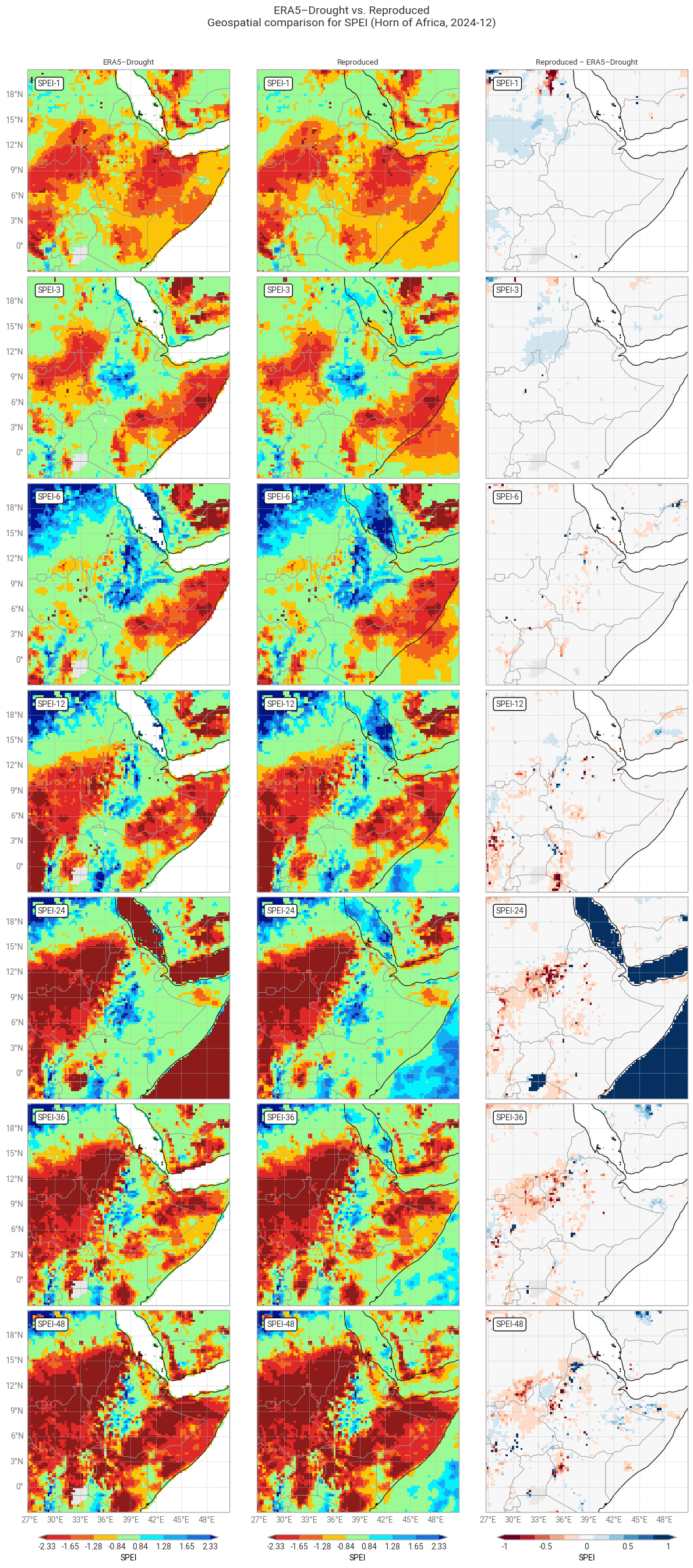
Fig. 6.1.13 SPEI downloaded from ERA5–Drought (left) vs. reproduced from ERA5 precipitation data (middle) and the difference between the two (right), for the region around the example site of Addis Ababa, Ethiopia. Only one month (December 2024) is displayed. Colours correspond to SPEI categories (e.g. “extremely dry”) in [Keune+25].

Confusion matrix

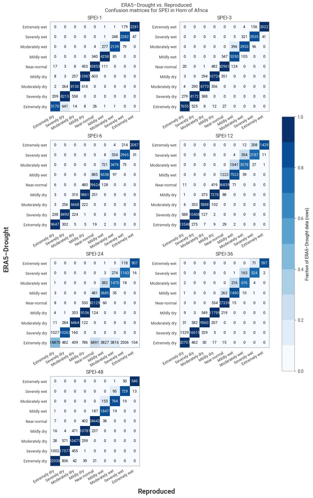
Fig. 6.1.14 Confusion matrices for SPEI categories from ERA5–Drought vs. reproduced from ERA5, across the region around the example site of Addis Ababa, Ethiopia. Combines data for all months within one year (2024).

4.6 Quality flags: Shapiro–Wilk normality test

ERA5–Drought includes one quality flag for SPEI, namely the normality α, derived using the Shapiro–Wilk test [Shapiro+65]. This α quantifies how well the computed SPI or SPEI values in the reference period (1991–2020) are described by a standard normal distribution. As such, α is provided for each combination of calendar month and accumulation window, for each pixel. The mask in ERA–Drought uses a threshold of 0.05, meaning points where α < 0.05 are rejected.

In this subsection, we reproduce the α quality flag mask, and compare its values to those provided in ERA5–Drought. Because this involves computing SPEI, which is computationally expensive, the evaluation is performed over the example region (Horn of Africa) rather than globally.

Show code cell source

Hide code cell source

# Select only desired site
data_era5_waterbalance_region = data_era5_waterbalance_preprocessed.sel(**example_region)

# Calculate SPEI
spei_reproduced_region = calculate_spei_from_era5(data_era5_waterbalance_region, reference_window=reference_window,
                                                  evaluation_window=reference_window)

Show code cell source

Hide code cell source

# Apply Shapiro–Wilk normality test
normality_reproduced = shapiro_wilk_normality(spei_reproduced_region)

# Retain in memory
normality_reproduced = normality_reproduced.persist()

# Create mask from normality p-values
# True: above threshold, allowed
# False: below threshold, flagged
normality_reproduced_mask = (normality_reproduced >= 0.05)

# Display result
normality_reproduced_mask

Show code cell output

Hide code cell output

<xarray.Dataset> Size: 792kB
Dimensions:  (lat: 97, lon: 97, month: 12)
Coordinates:
    number   int64 8B 0
  * lat      (lat) float64 776B 21.0 20.75 20.5 20.25 ... -2.25 -2.5 -2.75 -3.0
  * lon      (lon) float64 776B 26.75 27.0 27.25 27.5 ... 50.0 50.25 50.5 50.75
  * month    (month) int64 96B 1 2 3 4 5 6 7 8 9 10 11 12
Data variables:
    SPEI1    (month, lat, lon) bool 113kB dask.array<chunksize=(1, 33, 97), meta=np.ndarray>
    SPEI3    (month, lat, lon) bool 113kB dask.array<chunksize=(1, 33, 97), meta=np.ndarray>
    SPEI6    (month, lat, lon) bool 113kB dask.array<chunksize=(1, 33, 97), meta=np.ndarray>
    SPEI12   (month, lat, lon) bool 113kB dask.array<chunksize=(1, 33, 97), meta=np.ndarray>
    SPEI24   (month, lat, lon) bool 113kB dask.array<chunksize=(1, 33, 97), meta=np.ndarray>
    SPEI36   (month, lat, lon) bool 113kB dask.array<chunksize=(1, 33, 97), meta=np.ndarray>
    SPEI48   (month, lat, lon) bool 113kB dask.array<chunksize=(1, 33, 97), meta=np.ndarray>

xarray.Dataset

• Dimensions:
  • lat: 97
  • lon: 97
  • month: 12
• Coordinates: (4)
  • number
    ()
    int64
    0

    long_name :

    ensemble member numerical id

    units :

    1

    standard_name :

    realization

    array(0)

  • lat
    (lat)
    float64
    21.0 20.75 20.5 ... -2.5 -2.75 -3.0

    units :

    degrees_north

    standard_name :

    latitude

    long_name :

    latitude

    stored_direction :

    decreasing

    array([21.  , 20.75, 20.5 , 20.25, 20.  , 19.75, 19.5 , 19.25, 19.  , 18.75,
           18.5 , 18.25, 18.  , 17.75, 17.5 , 17.25, 17.  , 16.75, 16.5 , 16.25,
           16.  , 15.75, 15.5 , 15.25, 15.  , 14.75, 14.5 , 14.25, 14.  , 13.75,
           13.5 , 13.25, 13.  , 12.75, 12.5 , 12.25, 12.  , 11.75, 11.5 , 11.25,
           11.  , 10.75, 10.5 , 10.25, 10.  ,  9.75,  9.5 ,  9.25,  9.  ,  8.75,
            8.5 ,  8.25,  8.  ,  7.75,  7.5 ,  7.25,  7.  ,  6.75,  6.5 ,  6.25,
            6.  ,  5.75,  5.5 ,  5.25,  5.  ,  4.75,  4.5 ,  4.25,  4.  ,  3.75,
            3.5 ,  3.25,  3.  ,  2.75,  2.5 ,  2.25,  2.  ,  1.75,  1.5 ,  1.25,
            1.  ,  0.75,  0.5 ,  0.25,  0.  , -0.25, -0.5 , -0.75, -1.  , -1.25,
           -1.5 , -1.75, -2.  , -2.25, -2.5 , -2.75, -3.  ])

  • lon
    (lon)
    float64
    26.75 27.0 27.25 ... 50.5 50.75

    array([26.75, 27.  , 27.25, 27.5 , 27.75, 28.  , 28.25, 28.5 , 28.75, 29.  ,
           29.25, 29.5 , 29.75, 30.  , 30.25, 30.5 , 30.75, 31.  , 31.25, 31.5 ,
           31.75, 32.  , 32.25, 32.5 , 32.75, 33.  , 33.25, 33.5 , 33.75, 34.  ,
           34.25, 34.5 , 34.75, 35.  , 35.25, 35.5 , 35.75, 36.  , 36.25, 36.5 ,
           36.75, 37.  , 37.25, 37.5 , 37.75, 38.  , 38.25, 38.5 , 38.75, 39.  ,
           39.25, 39.5 , 39.75, 40.  , 40.25, 40.5 , 40.75, 41.  , 41.25, 41.5 ,
           41.75, 42.  , 42.25, 42.5 , 42.75, 43.  , 43.25, 43.5 , 43.75, 44.  ,
           44.25, 44.5 , 44.75, 45.  , 45.25, 45.5 , 45.75, 46.  , 46.25, 46.5 ,
           46.75, 47.  , 47.25, 47.5 , 47.75, 48.  , 48.25, 48.5 , 48.75, 49.  ,
           49.25, 49.5 , 49.75, 50.  , 50.25, 50.5 , 50.75])

  • month
    (month)
    int64
    1 2 3 4 5 6 7 8 9 10 11 12

    long_name :

    time

    standard_name :

    time

    array([ 1,  2,  3,  4,  5,  6,  7,  8,  9, 10, 11, 12])

• Data variables: (7)
  • SPEI1
    (month, lat, lon)
    bool
    dask.array<chunksize=(1, 33, 97), meta=np.ndarray>

    Array Chunk Bytes 110.26 kiB 6.06 kiB Shape (12, 97, 97) (1, 64, 97) Dask graph 24 chunks in 2 graph layers Data type bool numpy.ndarray

  • SPEI3
    (month, lat, lon)
    bool
    dask.array<chunksize=(1, 33, 97), meta=np.ndarray>

    Array Chunk Bytes 110.26 kiB 6.06 kiB Shape (12, 97, 97) (1, 64, 97) Dask graph 24 chunks in 2 graph layers Data type bool numpy.ndarray

  • SPEI6
    (month, lat, lon)
    bool
    dask.array<chunksize=(1, 33, 97), meta=np.ndarray>

    Array Chunk Bytes 110.26 kiB 6.06 kiB Shape (12, 97, 97) (1, 64, 97) Dask graph 24 chunks in 2 graph layers Data type bool numpy.ndarray

  • SPEI12
    (month, lat, lon)
    bool
    dask.array<chunksize=(1, 33, 97), meta=np.ndarray>

    Array Chunk Bytes 110.26 kiB 6.06 kiB Shape (12, 97, 97) (1, 64, 97) Dask graph 24 chunks in 2 graph layers Data type bool numpy.ndarray

  • SPEI24
    (month, lat, lon)
    bool
    dask.array<chunksize=(1, 33, 97), meta=np.ndarray>

    Array Chunk Bytes 110.26 kiB 6.06 kiB Shape (12, 97, 97) (1, 64, 97) Dask graph 24 chunks in 2 graph layers Data type bool numpy.ndarray

  • SPEI36
    (month, lat, lon)
    bool
    dask.array<chunksize=(1, 33, 97), meta=np.ndarray>

    Array Chunk Bytes 110.26 kiB 6.06 kiB Shape (12, 97, 97) (1, 64, 97) Dask graph 24 chunks in 2 graph layers Data type bool numpy.ndarray

  • SPEI48
    (month, lat, lon)
    bool
    dask.array<chunksize=(1, 33, 97), meta=np.ndarray>

    Array Chunk Bytes 110.26 kiB 6.06 kiB Shape (12, 97, 97) (1, 64, 97) Dask graph 24 chunks in 2 graph layers Data type bool numpy.ndarray

• Indexes: (3)
  • lat
    PandasIndex

    PandasIndex(Index([ 21.0, 20.75,  20.5, 20.25,  20.0, 19.75,  19.5, 19.25,  19.0, 18.75,
            18.5, 18.25,  18.0, 17.75,  17.5, 17.25,  17.0, 16.75,  16.5, 16.25,
            16.0, 15.75,  15.5, 15.25,  15.0, 14.75,  14.5, 14.25,  14.0, 13.75,
            13.5, 13.25,  13.0, 12.75,  12.5, 12.25,  12.0, 11.75,  11.5, 11.25,
            11.0, 10.75,  10.5, 10.25,  10.0,  9.75,   9.5,  9.25,   9.0,  8.75,
             8.5,  8.25,   8.0,  7.75,   7.5,  7.25,   7.0,  6.75,   6.5,  6.25,
             6.0,  5.75,   5.5,  5.25,   5.0,  4.75,   4.5,  4.25,   4.0,  3.75,
             3.5,  3.25,   3.0,  2.75,   2.5,  2.25,   2.0,  1.75,   1.5,  1.25,
             1.0,  0.75,   0.5,  0.25,   0.0, -0.25,  -0.5, -0.75,  -1.0, -1.25,
            -1.5, -1.75,  -2.0, -2.25,  -2.5, -2.75,  -3.0],
          dtype='float64', name='lat'))

  • lon
    PandasIndex

    PandasIndex(Index([26.75,  27.0, 27.25,  27.5, 27.75,  28.0, 28.25,  28.5, 28.75,  29.0,
           29.25,  29.5, 29.75,  30.0, 30.25,  30.5, 30.75,  31.0, 31.25,  31.5,
           31.75,  32.0, 32.25,  32.5, 32.75,  33.0, 33.25,  33.5, 33.75,  34.0,
           34.25,  34.5, 34.75,  35.0, 35.25,  35.5, 35.75,  36.0, 36.25,  36.5,
           36.75,  37.0, 37.25,  37.5, 37.75,  38.0, 38.25,  38.5, 38.75,  39.0,
           39.25,  39.5, 39.75,  40.0, 40.25,  40.5, 40.75,  41.0, 41.25,  41.5,
           41.75,  42.0, 42.25,  42.5, 42.75,  43.0, 43.25,  43.5, 43.75,  44.0,
           44.25,  44.5, 44.75,  45.0, 45.25,  45.5, 45.75,  46.0, 46.25,  46.5,
           46.75,  47.0, 47.25,  47.5, 47.75,  48.0, 48.25,  48.5, 48.75,  49.0,
           49.25,  49.5, 49.75,  50.0, 50.25,  50.5, 50.75],
          dtype='float64', name='lon'))

  • month
    PandasIndex

    PandasIndex(Index([1, 2, 3, 4, 5, 6, 7, 8, 9, 10, 11, 12], dtype='int64', name='month'))

• Attributes: (0)

The CDS provides ERA5–Drought’s α flag for each accumulation period, but does not distinguish between them in the variable name. This means that α must be downloaded separately for each accumulation period, renamed, and merged together, rather than downloading it for all simultaneously. Note that unlike for p₀, ERA5–Drought does not provide the value of α, only the corresponding boolean mask.

Show code cell source

Hide code cell source

# Setup: Request for each accumulation period
request_normality = {
    "variable": ["test_for_normality_spei"],
} | request_region | request_era5drought_flag

requests_per_accumulation_period = {period: {"accumulation_period": [str(period)],}
                                    for period in ACCUMULATION_PERIODS}

subrequests_era5drought_normality = {period: (req | request_normality)
                                       for period, req in requests_per_accumulation_period.items()}

# Download data in individual requests
normality_era5drought_mask = {period: ekd.from_source("cds", ID_ERA5_DROUGHT, subreq)  # Download as field lists
                              for period, subreq in subrequests_era5drought_normality.items()}

# Pre-process: Convert to xarray, handle variable names, month dimension
normality_era5drought_mask = preprocess_era5drought_qualityflag(normality_era5drought_mask, "SPEI")
normality_era5drought_mask = normality_era5drought_mask.astype(bool)  # Convert to boolean array (values are only 0. or 1.)

# Display in notebook
normality_era5drought_mask

Show code cell output

Hide code cell output

<xarray.Dataset> Size: 792kB
Dimensions:  (month: 12, lat: 97, lon: 97)
Coordinates:
    time     (month) datetime64[ns] 96B 2020-01-01 2020-02-01 ... 2020-12-01
  * lon      (lon) float64 776B 26.75 27.0 27.25 27.5 ... 50.0 50.25 50.5 50.75
  * lat      (lat) float64 776B 21.0 20.75 20.5 20.25 ... -2.25 -2.5 -2.75 -3.0
  * month    (month) int64 96B 1 2 3 4 5 6 7 8 9 10 11 12
Data variables:
    SPEI1    (month, lat, lon) bool 113kB dask.array<chunksize=(1, 97, 97), meta=np.ndarray>
    SPEI3    (month, lat, lon) bool 113kB dask.array<chunksize=(1, 97, 97), meta=np.ndarray>
    SPEI6    (month, lat, lon) bool 113kB dask.array<chunksize=(1, 97, 97), meta=np.ndarray>
    SPEI12   (month, lat, lon) bool 113kB dask.array<chunksize=(1, 97, 97), meta=np.ndarray>
    SPEI24   (month, lat, lon) bool 113kB dask.array<chunksize=(1, 97, 97), meta=np.ndarray>
    SPEI36   (month, lat, lon) bool 113kB dask.array<chunksize=(1, 97, 97), meta=np.ndarray>
    SPEI48   (month, lat, lon) bool 113kB dask.array<chunksize=(1, 97, 97), meta=np.ndarray>
Attributes: (12/19)
    CDI:                     Climate Data Interface version 1.9.10 (https://m...
    Conventions:             CF-1.8
    source:                  DRYFALL v1.0
    institution:             European Centre for Medium-Range Weather Forecasts
    title:                   Quality criteria for the derived standardized dr...
    description:             Monthly quality criteria that define the reliabi...
    ...                      ...
    resolution:              0.25x0.25
    climate_start_date:      1991-01-01
    climate_end_date:        2020-12-31
    frequency:               Monthly
    contact_person:          support@ecmwf.int
    CDO:                     Climate Data Operators version 1.9.10 (https://m...

xarray.Dataset

• Dimensions:
  • month: 12
  • lat: 97
  • lon: 97
• Coordinates: (4)
  • time
    (month)
    datetime64[ns]
    2020-01-01 ... 2020-12-01

    standard_name :

    time

    axis :

    T

    array(['2020-01-01T00:00:00.000000000', '2020-02-01T00:00:00.000000000',
           '2020-03-01T00:00:00.000000000', '2020-04-01T00:00:00.000000000',
           '2020-05-01T00:00:00.000000000', '2020-06-01T00:00:00.000000000',
           '2020-07-01T00:00:00.000000000', '2020-08-01T00:00:00.000000000',
           '2020-09-01T00:00:00.000000000', '2020-10-01T00:00:00.000000000',
           '2020-11-01T00:00:00.000000000', '2020-12-01T00:00:00.000000000'],
          dtype='datetime64[ns]')

  • lon
    (lon)
    float64
    26.75 27.0 27.25 ... 50.5 50.75

    standard_name :

    longitude

    long_name :

    longitude

    units :

    degrees_east

    axis :

    X

    array([26.75, 27.  , 27.25, 27.5 , 27.75, 28.  , 28.25, 28.5 , 28.75, 29.  ,
           29.25, 29.5 , 29.75, 30.  , 30.25, 30.5 , 30.75, 31.  , 31.25, 31.5 ,
           31.75, 32.  , 32.25, 32.5 , 32.75, 33.  , 33.25, 33.5 , 33.75, 34.  ,
           34.25, 34.5 , 34.75, 35.  , 35.25, 35.5 , 35.75, 36.  , 36.25, 36.5 ,
           36.75, 37.  , 37.25, 37.5 , 37.75, 38.  , 38.25, 38.5 , 38.75, 39.  ,
           39.25, 39.5 , 39.75, 40.  , 40.25, 40.5 , 40.75, 41.  , 41.25, 41.5 ,
           41.75, 42.  , 42.25, 42.5 , 42.75, 43.  , 43.25, 43.5 , 43.75, 44.  ,
           44.25, 44.5 , 44.75, 45.  , 45.25, 45.5 , 45.75, 46.  , 46.25, 46.5 ,
           46.75, 47.  , 47.25, 47.5 , 47.75, 48.  , 48.25, 48.5 , 48.75, 49.  ,
           49.25, 49.5 , 49.75, 50.  , 50.25, 50.5 , 50.75])

  • lat
    (lat)
    float64
    21.0 20.75 20.5 ... -2.5 -2.75 -3.0

    standard_name :

    latitude

    long_name :

    latitude

    units :

    degrees_north

    axis :

    Y

    array([21.  , 20.75, 20.5 , 20.25, 20.  , 19.75, 19.5 , 19.25, 19.  , 18.75,
           18.5 , 18.25, 18.  , 17.75, 17.5 , 17.25, 17.  , 16.75, 16.5 , 16.25,
           16.  , 15.75, 15.5 , 15.25, 15.  , 14.75, 14.5 , 14.25, 14.  , 13.75,
           13.5 , 13.25, 13.  , 12.75, 12.5 , 12.25, 12.  , 11.75, 11.5 , 11.25,
           11.  , 10.75, 10.5 , 10.25, 10.  ,  9.75,  9.5 ,  9.25,  9.  ,  8.75,
            8.5 ,  8.25,  8.  ,  7.75,  7.5 ,  7.25,  7.  ,  6.75,  6.5 ,  6.25,
            6.  ,  5.75,  5.5 ,  5.25,  5.  ,  4.75,  4.5 ,  4.25,  4.  ,  3.75,
            3.5 ,  3.25,  3.  ,  2.75,  2.5 ,  2.25,  2.  ,  1.75,  1.5 ,  1.25,
            1.  ,  0.75,  0.5 ,  0.25,  0.  , -0.25, -0.5 , -0.75, -1.  , -1.25,
           -1.5 , -1.75, -2.  , -2.25, -2.5 , -2.75, -3.  ])

  • month
    (month)
    int64
    1 2 3 4 5 6 7 8 9 10 11 12

    standard_name :

    time

    axis :

    T

    array([ 1,  2,  3,  4,  5,  6,  7,  8,  9, 10, 11, 12])

• Data variables: (7)
  • SPEI1
    (month, lat, lon)
    bool
    dask.array<chunksize=(1, 97, 97), meta=np.ndarray>

    long_name :

    Quality flag that indicates the acceptance of a Shapiro-Wilks test for normality using the derived standardized indices during the reference period; 1 indicates significant values and 0 indicates non-significant values at the alpha=0.05 level.

    units :

    1

    Array Chunk Bytes 110.26 kiB 9.19 kiB Shape (12, 97, 97) (1, 97, 97) Dask graph 12 chunks in 26 graph layers Data type bool numpy.ndarray

  • SPEI3
    (month, lat, lon)
    bool
    dask.array<chunksize=(1, 97, 97), meta=np.ndarray>

    long_name :

    Quality flag that indicates the acceptance of a Shapiro-Wilks test for normality using the derived standardized indices during the reference period; 1 indicates significant values and 0 indicates non-significant values at the alpha=0.05 level.

    units :

    1

    Array Chunk Bytes 110.26 kiB 9.19 kiB Shape (12, 97, 97) (1, 97, 97) Dask graph 12 chunks in 26 graph layers Data type bool numpy.ndarray

  • SPEI6
    (month, lat, lon)
    bool
    dask.array<chunksize=(1, 97, 97), meta=np.ndarray>

    long_name :

    Quality flag that indicates the acceptance of a Shapiro-Wilks test for normality using the derived standardized indices during the reference period; 1 indicates significant values and 0 indicates non-significant values at the alpha=0.05 level.

    units :

    1

    Array Chunk Bytes 110.26 kiB 9.19 kiB Shape (12, 97, 97) (1, 97, 97) Dask graph 12 chunks in 26 graph layers Data type bool numpy.ndarray

  • SPEI12
    (month, lat, lon)
    bool
    dask.array<chunksize=(1, 97, 97), meta=np.ndarray>

    long_name :

    Quality flag that indicates the acceptance of a Shapiro-Wilks test for normality using the derived standardized indices during the reference period; 1 indicates significant values and 0 indicates non-significant values at the alpha=0.05 level.

    units :

    1

    Array Chunk Bytes 110.26 kiB 9.19 kiB Shape (12, 97, 97) (1, 97, 97) Dask graph 12 chunks in 26 graph layers Data type bool numpy.ndarray

  • SPEI24
    (month, lat, lon)
    bool
    dask.array<chunksize=(1, 97, 97), meta=np.ndarray>

    long_name :

    Quality flag that indicates the acceptance of a Shapiro-Wilks test for normality using the derived standardized indices during the reference period; 1 indicates significant values and 0 indicates non-significant values at the alpha=0.05 level.

    units :

    1

    Array Chunk Bytes 110.26 kiB 9.19 kiB Shape (12, 97, 97) (1, 97, 97) Dask graph 12 chunks in 26 graph layers Data type bool numpy.ndarray

  • SPEI36
    (month, lat, lon)
    bool
    dask.array<chunksize=(1, 97, 97), meta=np.ndarray>

    long_name :

    Quality flag that indicates the acceptance of a Shapiro-Wilks test for normality using the derived standardized indices during the reference period; 1 indicates significant values and 0 indicates non-significant values at the alpha=0.05 level.

    units :

    1

    Array Chunk Bytes 110.26 kiB 9.19 kiB Shape (12, 97, 97) (1, 97, 97) Dask graph 12 chunks in 26 graph layers Data type bool numpy.ndarray

  • SPEI48
    (month, lat, lon)
    bool
    dask.array<chunksize=(1, 97, 97), meta=np.ndarray>

    long_name :

    Quality flag that indicates the acceptance of a Shapiro-Wilks test for normality using the derived standardized indices during the reference period; 1 indicates significant values and 0 indicates non-significant values at the alpha=0.05 level.

    units :

    1

    Array Chunk Bytes 110.26 kiB 9.19 kiB Shape (12, 97, 97) (1, 97, 97) Dask graph 12 chunks in 26 graph layers Data type bool numpy.ndarray

• Indexes: (3)
  • lon
    PandasIndex

    PandasIndex(Index([26.75,  27.0, 27.25,  27.5, 27.75,  28.0, 28.25,  28.5, 28.75,  29.0,
           29.25,  29.5, 29.75,  30.0, 30.25,  30.5, 30.75,  31.0, 31.25,  31.5,
           31.75,  32.0, 32.25,  32.5, 32.75,  33.0, 33.25,  33.5, 33.75,  34.0,
           34.25,  34.5, 34.75,  35.0, 35.25,  35.5, 35.75,  36.0, 36.25,  36.5,
           36.75,  37.0, 37.25,  37.5, 37.75,  38.0, 38.25,  38.5, 38.75,  39.0,
           39.25,  39.5, 39.75,  40.0, 40.25,  40.5, 40.75,  41.0, 41.25,  41.5,
           41.75,  42.0, 42.25,  42.5, 42.75,  43.0, 43.25,  43.5, 43.75,  44.0,
           44.25,  44.5, 44.75,  45.0, 45.25,  45.5, 45.75,  46.0, 46.25,  46.5,
           46.75,  47.0, 47.25,  47.5, 47.75,  48.0, 48.25,  48.5, 48.75,  49.0,
           49.25,  49.5, 49.75,  50.0, 50.25,  50.5, 50.75],
          dtype='float64', name='lon'))

  • lat
    PandasIndex

    PandasIndex(Index([ 21.0, 20.75,  20.5, 20.25,  20.0, 19.75,  19.5, 19.25,  19.0, 18.75,
            18.5, 18.25,  18.0, 17.75,  17.5, 17.25,  17.0, 16.75,  16.5, 16.25,
            16.0, 15.75,  15.5, 15.25,  15.0, 14.75,  14.5, 14.25,  14.0, 13.75,
            13.5, 13.25,  13.0, 12.75,  12.5, 12.25,  12.0, 11.75,  11.5, 11.25,
            11.0, 10.75,  10.5, 10.25,  10.0,  9.75,   9.5,  9.25,   9.0,  8.75,
             8.5,  8.25,   8.0,  7.75,   7.5,  7.25,   7.0,  6.75,   6.5,  6.25,
             6.0,  5.75,   5.5,  5.25,   5.0,  4.75,   4.5,  4.25,   4.0,  3.75,
             3.5,  3.25,   3.0,  2.75,   2.5,  2.25,   2.0,  1.75,   1.5,  1.25,
             1.0,  0.75,   0.5,  0.25,   0.0, -0.25,  -0.5, -0.75,  -1.0, -1.25,
            -1.5, -1.75,  -2.0, -2.25,  -2.5, -2.75,  -3.0],
          dtype='float64', name='lat'))

  • month
    PandasIndex

    PandasIndex(Index([1, 2, 3, 4, 5, 6, 7, 8, 9, 10, 11, 12], dtype='int64', name='month'))

• Attributes: (19)

  CDI :

  Climate Data Interface version 1.9.10 (https://mpimet.mpg.de/cdi)

  Conventions :

  CF-1.8

  source :

  DRYFALL v1.0

  institution :

  European Centre for Medium-Range Weather Forecasts

  title :

  Quality criteria for the derived standardized drought indices

  description :

  Monthly quality criteria that define the reliability of the derived drought indices.

  history :

  Tue Aug 13 11:21:50 2024: cdo -selvar,significance -setdate,20200101 -seldate,19000101 /ec/ws4/tc/emos/work/cems/dryfall/emos/dryfall_monthly/generated_climate/parameters/SPEI1_genlogistic_global_era5_moda_ref1991to2020_params.nc SPEI1_speisignificance_genlogistic_global_era5_moda_ref1991to2020_01.nc Created 13/08/2024 11:20:58 using DRYFALL.

  license :

  Creative Commons Attribution v4

  citation_statement :

  Drought indicators derived from ERA5 reanalysis

  ref_publication :

  Keune, J., F. Di Giuseppe, C. Barnard, D. Damasio da Costa, and F. Wetterhall: ERA5–Drought: Global drought indicators based on ECMWF reanalysis.

  cds_data_catalogue_url :

  https://ecds.climate.copernicus.eu/datasets/derived-drought-historical

  data_srs :

  EPSG:4326

  extent :

  -180,-90,180,90

  resolution :

  0.25x0.25

  climate_start_date :

  1991-01-01

  climate_end_date :

  2020-12-31

  frequency :

  Monthly

  contact_person :

  support@ecmwf.int

  CDO :

  Climate Data Operators version 1.9.10 (https://mpimet.mpg.de/cdo)

First, we quantitatively compare how often the values of the normality mask desired from α in ERA5–Drought and the reproduction match:

Show code cell source

Hide code cell source

# Package probability and masks into dictionary for table function; note use unicode symbols / HTML
normality_flags = {"α < 0.05 [%]": [normality_reproduced_mask, normality_era5drought_mask],
                  }
        
# Compare probabilities per variable
compare_quality_flags(normality_flags, title_suffix=f" ({domain_region.name})")

ERA5–Drought vs. Reproduced Quality flag matches (Horn of Africa)

	SPEI-1	SPEI-3	SPEI-6	SPEI-12	SPEI-24	SPEI-36	SPEI-48
Matching α < 0.05 [%]	92.77	91.43	90.64	91.13	88.83	87.77	87.51

Agreement in the SPEI normality flag is excellent (≥87%) across all accumulation periods. The normality mask is applied much more rarely for SPEI than for SPI and mismatched months appear randomly distributed across the Horn region (Figures 6.1.15 and 6.1.16). This result shows that while the fitted distributions themselves may differ between ERA5–Drought and the reproduction, they tend to either both pass or both fail the normality test.

Show code cell source

Hide code cell source

# Package masks into dictionary for plotting function; note use of LaTeX instead of unicode/HTML symbols
masks = {r"$\alpha < 0.05$": [normality_era5drought_mask, normality_reproduced_mask],
        }

# Display quality flags – this step may take a few minutes
# SPI-1: Compare to table
plot_geospatial_comparison_quality_flags("SPEI1", masks=masks,
                                         shared_mask=LAND, domain=domain_region,
                                         glue_label="indicator_derived-drought-historical-monthly_consistency_q01_fig-spei-normality-region-spei1")

# SPI-3: Compare to Keune+25 Fig 3.
plot_geospatial_comparison_quality_flags("SPEI3", masks=masks,
                                         shared_mask=LAND, domain=domain_region,
                                         glue_label="indicator_derived-drought-historical-monthly_consistency_q01_fig-spei-normality-region-spei3")

SPEI-1

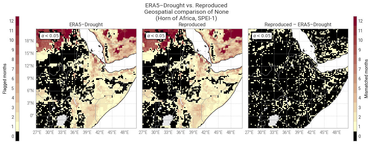
Fig. 6.1.15 Shapiro–Wilk normality α for SPEI-1 and associated masks in ERA5–Drought (left) vs. reproduced from ERA5 precipitation data (middle) and the difference or mismatch between the two (right). The α < 0.05 mask is displayed as the number of calendar months that get flagged and the oceans are masked, following [Keune+25] Fig. 3. This figure displays only the example region (Horn of Africa).

SPEI-3

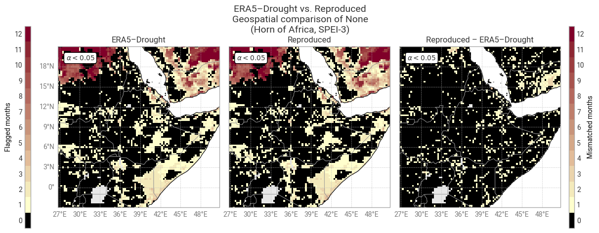
Fig. 6.1.16 Shapiro–Wilk normality α for SPEI-3 and associated masks in ERA5–Drought (left) vs. reproduced from ERA5 precipitation data (middle) and the difference or mismatch between the two (right). The α < 0.05 mask is displayed as the number of calendar months that get flagged and the oceans are masked, following [Keune+25] Fig. 3. This figure displays only the example region (Horn of Africa).

5. Ensemble comparison

One of the key strengths of ERA5–Drought is its inclusion of 10 ensemble members, propagated from ERA5, which can be used to probe (part of) the uncertainty in SPI and SPEI values [Keune+25].

Here, we briefly demonstrate the reproducibility of the ERA5–Drought ensemble from the corresponding ERA5 ensemble members. To avoid repetition and reduce computational cost – since the ensemble dataset is 10× the size of the reanalysis – this section focuses on the case study of SPI and SPEI in one site. If you are keen to investigate the reproducibility of the ERA5–Drought ensemble more, the code provided in this notebook can easily be re-used to do so.

5.1 Compute SPI and SPEI from ERA5 ensemble

As before, precipitation and potential evaporation are downloaded from the Complete ERA5 global atmospheric reanalysis dataset, but this time using the edmo (monthly ensemble) stream. The ERA5 ensemble is provided at a coarser resolution than the main reanalysis; ERA5–Drought regrids both to the same 0.25° by 0.25° grid, which we do here using MARS’s internal functionalities. In code, this is implemented through the line "grid": "0.25/0.25", in the ERA5 request (request_era5_template).

Show code cell source

Hide code cell source

request_era5_precipitation_edmo = {
    "param": "228.128",       # Variable: Total precipitation
    "stream": "edmo",         # Data stream: Monthly mean reanalysis
} | request_era5_template

request_era5_evaporation_edmo = {
    "param": "251.228", # Variable: Total potential evaporation.
    "stream": "edmo",  # Data stream: Monthly mean reanalysis
} | request_era5_template

Show code cell source

Hide code cell source

# Download data and load into xarray
data_era5_waterbalance_ensemble_cds = ekd.from_source("cds", ID_ERA5, request_era5_precipitation_edmo,
                                                      request_era5_evaporation_edmo)  # Download as field list

data_era5_waterbalance_ensemble_cds = data_era5_waterbalance_ensemble_cds.to_xarray(compat="equals")  # Convert to xarray dataset

# Pre-process to desired format
# Note the change in variable name
data_era5_waterbalance_ensemble_preprocessed = preprocess_era5(data_era5_waterbalance_ensemble_cds)

# Display in notebook, both "tp" and "pev".
data_era5_waterbalance_ensemble_preprocessed 

Show code cell output

Hide code cell output

<xarray.Dataset> Size: 85GB
Dimensions:  (number: 10, time: 1020, lat: 721, lon: 1440)
Coordinates:
  * number   (number) int64 80B 0 1 2 3 4 5 6 7 8 9
  * time     (time) datetime64[ns] 8kB 1940-01-01T06:00:00 ... 2024-12-01T06:...
  * lat      (lat) float64 6kB 90.0 89.75 89.5 89.25 ... -89.5 -89.75 -90.0
    expver   (time) <U4 16kB dask.array<chunksize=(1020,), meta=np.ndarray>
  * lon      (lon) float64 12kB -180.0 -179.8 -179.5 ... 179.2 179.5 179.8
Data variables:
    tp       (number, time, lat, lon) float32 42GB dask.array<chunksize=(1, 1020, 103, 360), meta=np.ndarray>
    pev      (number, time, lat, lon) float32 42GB dask.array<chunksize=(1, 1020, 103, 360), meta=np.ndarray>
Attributes:
    GRIB_centre:             ecmf
    GRIB_centreDescription:  European Centre for Medium-Range Weather Forecasts
    GRIB_subCentre:          0
    Conventions:             CF-1.7
    institution:             European Centre for Medium-Range Weather Forecasts

xarray.Dataset

• Dimensions:
  • number: 10
  • time: 1020
  • lat: 721
  • lon: 1440
• Coordinates: (5)
  • number
    (number)
    int64
    0 1 2 3 4 5 6 7 8 9

    long_name :

    ensemble member numerical id

    units :

    1

    standard_name :

    realization

    array([0, 1, 2, 3, 4, 5, 6, 7, 8, 9])

  • time
    (time)
    datetime64[ns]
    1940-01-01T06:00:00 ... 2024-12-...

    long_name :

    time

    standard_name :

    time

    array(['1940-01-01T06:00:00.000000000', '1940-02-01T06:00:00.000000000',
           '1940-03-01T06:00:00.000000000', ..., '2024-10-01T06:00:00.000000000',
           '2024-11-01T06:00:00.000000000', '2024-12-01T06:00:00.000000000'],
          shape=(1020,), dtype='datetime64[ns]')

  • lat
    (lat)
    float64
    90.0 89.75 89.5 ... -89.75 -90.0

    units :

    degrees_north

    standard_name :

    latitude

    long_name :

    latitude

    stored_direction :

    decreasing

    array([ 90.  ,  89.75,  89.5 , ..., -89.5 , -89.75, -90.  ], shape=(721,))

  • expver
    (time)
    <U4
    dask.array<chunksize=(1020,), meta=np.ndarray>

    Array Chunk Bytes 15.94 kiB 15.94 kiB Shape (1020,) (1020,) Dask graph 1 chunks in 1 graph layer Data type

  • lon
    (lon)
    float64
    -180.0 -179.8 ... 179.5 179.8

    array([-180.  , -179.75, -179.5 , ...,  179.25,  179.5 ,  179.75],
          shape=(1440,))

• Data variables: (2)
  • tp
    (number, time, lat, lon)
    float32
    dask.array<chunksize=(1, 1020, 103, 360), meta=np.ndarray>

    GRIB_paramId :

    228

    GRIB_dataType :

    fc

    GRIB_numberOfPoints :

    1038240

    GRIB_typeOfLevel :

    surface

    GRIB_stepUnits :

    1

    GRIB_stepType :

    avgad

    GRIB_gridType :

    regular_ll

    GRIB_uvRelativeToGrid :

    0

    GRIB_NV :

    0

    GRIB_Nx :

    1440

    GRIB_Ny :

    721

    GRIB_cfName :

    unknown

    GRIB_cfVarName :

    tp

    GRIB_gridDefinitionDescription :

    Latitude/Longitude Grid

    GRIB_iDirectionIncrementInDegrees :

    0.25

    GRIB_iScansNegatively :

    0

    GRIB_jDirectionIncrementInDegrees :

    0.25

    GRIB_jPointsAreConsecutive :

    0

    GRIB_jScansPositively :

    0

    GRIB_latitudeOfFirstGridPointInDegrees :

    90.0

    GRIB_latitudeOfLastGridPointInDegrees :

    -90.0

    GRIB_longitudeOfFirstGridPointInDegrees :

    0.0

    GRIB_longitudeOfLastGridPointInDegrees :

    359.75

    GRIB_missingValue :

    3.4028234663852886e+38

    GRIB_name :

    Total precipitation

    GRIB_shortName :

    tp

    GRIB_totalNumber :

    10

    GRIB_units :

    m

    long_name :

    Total precipitation

    units :

    mm

    standard_name :

    unknown

    GRIB_surface :

    0.0

    Array Chunk Bytes 39.45 GiB 144.28 MiB Shape (10, 1020, 721, 1440) (1, 1020, 103, 360) Dask graph 280 chunks in 5 graph layers Data type float32 numpy.ndarray

  • pev
    (number, time, lat, lon)
    float32
    dask.array<chunksize=(1, 1020, 103, 360), meta=np.ndarray>

    GRIB_paramId :

    228251

    GRIB_dataType :

    fc

    GRIB_numberOfPoints :

    1038240

    GRIB_typeOfLevel :

    surface

    GRIB_stepUnits :

    1

    GRIB_stepType :

    avgad

    GRIB_gridType :

    regular_ll

    GRIB_uvRelativeToGrid :

    0

    GRIB_NV :

    0

    GRIB_Nx :

    1440

    GRIB_Ny :

    721

    GRIB_cfName :

    unknown

    GRIB_cfVarName :

    pev

    GRIB_gridDefinitionDescription :

    Latitude/Longitude Grid

    GRIB_iDirectionIncrementInDegrees :

    0.25

    GRIB_iScansNegatively :

    0

    GRIB_jDirectionIncrementInDegrees :

    0.25

    GRIB_jPointsAreConsecutive :

    0

    GRIB_jScansPositively :

    0

    GRIB_latitudeOfFirstGridPointInDegrees :

    90.0

    GRIB_latitudeOfLastGridPointInDegrees :

    -90.0

    GRIB_longitudeOfFirstGridPointInDegrees :

    0.0

    GRIB_longitudeOfLastGridPointInDegrees :

    359.75

    GRIB_missingValue :

    3.4028234663852886e+38

    GRIB_name :

    Potential evaporation

    GRIB_shortName :

    pev

    GRIB_totalNumber :

    10

    GRIB_units :

    m

    long_name :

    Potential evaporation

    units :

    mm

    standard_name :

    unknown

    GRIB_surface :

    0.0

    Array Chunk Bytes 39.45 GiB 144.28 MiB Shape (10, 1020, 721, 1440) (1, 1020, 103, 360) Dask graph 280 chunks in 5 graph layers Data type float32 numpy.ndarray

• Indexes: (4)
  • number
    PandasIndex

    PandasIndex(Index([0, 1, 2, 3, 4, 5, 6, 7, 8, 9], dtype='int64', name='number'))

  • time
    PandasIndex

    PandasIndex(DatetimeIndex(['1940-01-01 06:00:00', '1940-02-01 06:00:00',
                   '1940-03-01 06:00:00', '1940-04-01 06:00:00',
                   '1940-05-01 06:00:00', '1940-06-01 06:00:00',
                   '1940-07-01 06:00:00', '1940-08-01 06:00:00',
                   '1940-09-01 06:00:00', '1940-10-01 06:00:00',
                   ...
                   '2024-03-01 06:00:00', '2024-04-01 06:00:00',
                   '2024-05-01 06:00:00', '2024-06-01 06:00:00',
                   '2024-07-01 06:00:00', '2024-08-01 06:00:00',
                   '2024-09-01 06:00:00', '2024-10-01 06:00:00',
                   '2024-11-01 06:00:00', '2024-12-01 06:00:00'],
                  dtype='datetime64[ns]', name='time', length=1020, freq=None))

  • lat
    PandasIndex

    PandasIndex(Index([  90.0,  89.75,   89.5,  89.25,   89.0,  88.75,   88.5,  88.25,   88.0,
            87.75,
           ...
           -87.75,  -88.0, -88.25,  -88.5, -88.75,  -89.0, -89.25,  -89.5, -89.75,
            -90.0],
          dtype='float64', name='lat', length=721))

  • lon
    PandasIndex

    PandasIndex(Index([ -180.0, -179.75,  -179.5, -179.25,  -179.0, -178.75,  -178.5, -178.25,
            -178.0, -177.75,
           ...
             177.5,  177.75,   178.0,  178.25,   178.5,  178.75,   179.0,  179.25,
             179.5,  179.75],
          dtype='float64', name='lon', length=1440))

• Attributes: (5)

  GRIB_centre :

  ecmf

  GRIB_centreDescription :

  European Centre for Medium-Range Weather Forecasts

  GRIB_subCentre :

  0

  Conventions :

  CF-1.7

  institution :

  European Centre for Medium-Range Weather Forecasts

SPI and SPEI are calculated using the calculate_spi_from_era5 and calculate_spei_from_era5 functions defined in 1. Code setup. These functions handle the new number dimension by applying the full SPI / SPEI pipeline to each member independently, just like in ERA5–Drought.

Show code cell source

Hide code cell source

# Select only desired site
data_era5_waterbalance_ensemble_preprocessed_site = data_era5_waterbalance_ensemble_preprocessed.sel(**example_site)

# Calculate SPI for example site, for all members
spi_reproduced_site_ensemble = calculate_spi_from_era5(data_era5_waterbalance_ensemble_preprocessed_site,
                                                       reference_window=reference_window)

# Calculate SPI for example site, for all members
spei_reproduced_site_ensemble = calculate_spei_from_era5(data_era5_waterbalance_ensemble_preprocessed_site,
                                                         reference_window=reference_window)

# Display result
spei_reproduced_site_ensemble

<xarray.Dataset> Size: 604kB
Dimensions:  (number: 10, time: 1020)
Coordinates:
  * number   (number) int64 80B 0 1 2 3 4 5 6 7 8 9
  * time     (time) datetime64[ns] 8kB 1940-01-01T06:00:00 ... 2024-12-01T06:...
    lat      float64 8B 9.0
    expver   (time) <U4 16kB dask.array<chunksize=(1020,), meta=np.ndarray>
    lon      float64 8B 38.75
    month    (time) int64 8kB dask.array<chunksize=(1020,), meta=np.ndarray>
Data variables:
    SPEI1    (number, time) float64 82kB dask.array<chunksize=(1, 1020), meta=np.ndarray>
    SPEI3    (number, time) float64 82kB dask.array<chunksize=(1, 1020), meta=np.ndarray>
    SPEI6    (number, time) float64 82kB dask.array<chunksize=(1, 1020), meta=np.ndarray>
    SPEI12   (number, time) float64 82kB dask.array<chunksize=(1, 1020), meta=np.ndarray>
    SPEI24   (number, time) float64 82kB dask.array<chunksize=(1, 1020), meta=np.ndarray>
    SPEI36   (number, time) float64 82kB dask.array<chunksize=(1, 1020), meta=np.ndarray>
    SPEI48   (number, time) float64 82kB dask.array<chunksize=(1, 1020), meta=np.ndarray>

xarray.Dataset

• Dimensions:
  • number: 10
  • time: 1020
• Coordinates: (6)
  • number
    (number)
    int64
    0 1 2 3 4 5 6 7 8 9

    long_name :

    ensemble member numerical id

    units :

    1

    standard_name :

    realization

    array([0, 1, 2, 3, 4, 5, 6, 7, 8, 9])

  • time
    (time)
    datetime64[ns]
    1940-01-01T06:00:00 ... 2024-12-...

    long_name :

    time

    standard_name :

    time

    array(['1940-01-01T06:00:00.000000000', '1940-02-01T06:00:00.000000000',
           '1940-03-01T06:00:00.000000000', ..., '2024-10-01T06:00:00.000000000',
           '2024-11-01T06:00:00.000000000', '2024-12-01T06:00:00.000000000'],
          shape=(1020,), dtype='datetime64[ns]')

  • lat
    ()
    float64
    9.0

    units :

    degrees_north

    standard_name :

    latitude

    long_name :

    latitude

    stored_direction :

    decreasing

    array(9.)

  • expver
    (time)
    <U4
    dask.array<chunksize=(1020,), meta=np.ndarray>

    Array Chunk Bytes 15.94 kiB 15.94 kiB Shape (1020,) (1020,) Dask graph 1 chunks in 1 graph layer Data type

  • lon
    ()
    float64
    38.75

    array(38.75)

  • month
    (time)
    int64
    dask.array<chunksize=(1020,), meta=np.ndarray>

    long_name :

    time

    standard_name :

    time

    Array Chunk Bytes 7.97 kiB 7.97 kiB Shape (1020,) (1020,) Dask graph 1 chunks in 1 graph layer Data type int64 numpy.ndarray

• Data variables: (7)
  • SPEI1
    (number, time)
    float64
    dask.array<chunksize=(1, 1020), meta=np.ndarray>

    Array Chunk Bytes 79.69 kiB 7.97 kiB Shape (10, 1020) (1, 1020) Dask graph 10 chunks in 112 graph layers Data type float64 numpy.ndarray

  • SPEI3
    (number, time)
    float64
    dask.array<chunksize=(1, 1020), meta=np.ndarray>

    Array Chunk Bytes 79.69 kiB 7.97 kiB Shape (10, 1020) (1, 1020) Dask graph 10 chunks in 119 graph layers Data type float64 numpy.ndarray

  • SPEI6
    (number, time)
    float64
    dask.array<chunksize=(1, 1020), meta=np.ndarray>

    Array Chunk Bytes 79.69 kiB 7.97 kiB Shape (10, 1020) (1, 1020) Dask graph 10 chunks in 119 graph layers Data type float64 numpy.ndarray

  • SPEI12
    (number, time)
    float64
    dask.array<chunksize=(1, 1020), meta=np.ndarray>

    Array Chunk Bytes 79.69 kiB 7.97 kiB Shape (10, 1020) (1, 1020) Dask graph 10 chunks in 119 graph layers Data type float64 numpy.ndarray

  • SPEI24
    (number, time)
    float64
    dask.array<chunksize=(1, 1020), meta=np.ndarray>

    Array Chunk Bytes 79.69 kiB 7.97 kiB Shape (10, 1020) (1, 1020) Dask graph 10 chunks in 119 graph layers Data type float64 numpy.ndarray

  • SPEI36
    (number, time)
    float64
    dask.array<chunksize=(1, 1020), meta=np.ndarray>

    Array Chunk Bytes 79.69 kiB 7.97 kiB Shape (10, 1020) (1, 1020) Dask graph 10 chunks in 119 graph layers Data type float64 numpy.ndarray

  • SPEI48
    (number, time)
    float64
    dask.array<chunksize=(1, 1020), meta=np.ndarray>

    Array Chunk Bytes 79.69 kiB 7.97 kiB Shape (10, 1020) (1, 1020) Dask graph 10 chunks in 119 graph layers Data type float64 numpy.ndarray

• Indexes: (2)
  • number
    PandasIndex

    PandasIndex(Index([0, 1, 2, 3, 4, 5, 6, 7, 8, 9], dtype='int64', name='number'))

  • time
    PandasIndex

    PandasIndex(DatetimeIndex(['1940-01-01 06:00:00', '1940-02-01 06:00:00',
                   '1940-03-01 06:00:00', '1940-04-01 06:00:00',
                   '1940-05-01 06:00:00', '1940-06-01 06:00:00',
                   '1940-07-01 06:00:00', '1940-08-01 06:00:00',
                   '1940-09-01 06:00:00', '1940-10-01 06:00:00',
                   ...
                   '2024-03-01 06:00:00', '2024-04-01 06:00:00',
                   '2024-05-01 06:00:00', '2024-06-01 06:00:00',
                   '2024-07-01 06:00:00', '2024-08-01 06:00:00',
                   '2024-09-01 06:00:00', '2024-10-01 06:00:00',
                   '2024-11-01 06:00:00', '2024-12-01 06:00:00'],
                  dtype='datetime64[ns]', name='time', length=1020, freq=None))

• Attributes: (0)

5.2 Download SPI and SPEI ensembles from ERA5–Drought

Next, we download the SPI and SPEI ensemble data from ERA5–Drought. Unlike in ERA5, the ensemble is not represented through a separate number dimension, but instead using 10-duplicate entries in the time dimension. To simplify the analysis, we restructure the downloaded dataset to match ERA5’s setup:

Show code cell source

Hide code cell source

# Main request, based on template and example site
request_era5drought_spi_ensemble = {
    "variable": ["standardised_precipitation_index"],
} | request_era5drought_index_ensemble | request_site

request_era5drought_spei_ensemble = {
    "variable": ["standardised_precipitation_evapotranspiration_index"],
} | request_era5drought_index_ensemble | request_site

# Split into batches per accumulation period
subrequests_era5drought_spi_ensemble  = batch_requests(request_era5drought_spi_ensemble,  batch_key="accumulation_period", n=1)
subrequests_era5drought_spei_ensemble = batch_requests(request_era5drought_spei_ensemble, batch_key="accumulation_period", n=1)

Show code cell source

Hide code cell source

# Download SPI data and load into xarray
spi_era5drought_site_ensemble = ekd.from_source("cds", ID_ERA5_DROUGHT, *subrequests_era5drought_spi_ensemble)
spi_era5drought_site_ensemble = preprocess_era5drought_ensemble(spi_era5drought_site_ensemble)  # Handle number dimension, combine into one dataset

# Download SPEI data and load into xarray
spei_era5drought_site_ensemble = ekd.from_source("cds", ID_ERA5_DROUGHT, *subrequests_era5drought_spei_ensemble)
spei_era5drought_site_ensemble = preprocess_era5drought_ensemble(spei_era5drought_site_ensemble)  # Handle number dimension, combine into one dataset

# Select only desired site (remove margins)
spi_era5drought_site_ensemble  =  spi_era5drought_site_ensemble.sel(**example_site)
spei_era5drought_site_ensemble = spei_era5drought_site_ensemble.sel(**example_site)

# Display result
spei_era5drought_site_ensemble

Show code cell output

Hide code cell output

<xarray.Dataset> Size: 579kB
Dimensions:  (time: 1020, number: 10)
Coordinates:
  * time     (time) datetime64[ns] 8kB 1940-01-01T06:00:00 ... 2024-12-01T06:...
    lon      float64 8B 38.75
    lat      float64 8B 9.0
  * number   (number) int64 80B 0 1 2 3 4 5 6 7 8 9
Data variables:
    SPEI1    (number, time) float64 82kB dask.array<chunksize=(10, 1020), meta=np.ndarray>
    SPEI3    (number, time) float64 82kB dask.array<chunksize=(10, 1020), meta=np.ndarray>
    SPEI6    (number, time) float64 82kB dask.array<chunksize=(10, 1020), meta=np.ndarray>
    SPEI12   (number, time) float64 82kB dask.array<chunksize=(10, 1020), meta=np.ndarray>
    SPEI24   (number, time) float64 82kB dask.array<chunksize=(10, 1020), meta=np.ndarray>
    SPEI36   (number, time) float64 82kB dask.array<chunksize=(10, 1020), meta=np.ndarray>
    SPEI48   (number, time) float64 82kB dask.array<chunksize=(10, 1020), meta=np.ndarray>

xarray.Dataset

• Dimensions:
  • time: 1020
  • number: 10
• Coordinates: (4)
  • time
    (time)
    datetime64[ns]
    1940-01-01T06:00:00 ... 2024-12-...

    array(['1940-01-01T06:00:00.000000000', '1940-02-01T06:00:00.000000000',
           '1940-03-01T06:00:00.000000000', ..., '2024-10-01T06:00:00.000000000',
           '2024-11-01T06:00:00.000000000', '2024-12-01T06:00:00.000000000'],
          shape=(1020,), dtype='datetime64[ns]')

  • lon
    ()
    float64
    38.75

    array(38.75)

  • lat
    ()
    float64
    9.0

    array(9.)

  • number
    (number)
    int64
    0 1 2 3 4 5 6 7 8 9

    array([0, 1, 2, 3, 4, 5, 6, 7, 8, 9])

• Data variables: (7)
  • SPEI1
    (number, time)
    float64
    dask.array<chunksize=(10, 1020), meta=np.ndarray>

    Array Chunk Bytes 79.69 kiB 79.69 kiB Shape (10, 1020) (10, 1020) Dask graph 1 chunks in 1023 graph layers Data type float64 numpy.ndarray

  • SPEI3
    (number, time)
    float64
    dask.array<chunksize=(10, 1020), meta=np.ndarray>

    Array Chunk Bytes 79.69 kiB 79.69 kiB Shape (10, 1020) (10, 1020) Dask graph 1 chunks in 1035 graph layers Data type float64 numpy.ndarray

  • SPEI6
    (number, time)
    float64
    dask.array<chunksize=(10, 1020), meta=np.ndarray>

    Array Chunk Bytes 79.69 kiB 79.69 kiB Shape (10, 1020) (10, 1020) Dask graph 1 chunks in 1032 graph layers Data type float64 numpy.ndarray

  • SPEI12
    (number, time)
    float64
    dask.array<chunksize=(10, 1020), meta=np.ndarray>

    Array Chunk Bytes 79.69 kiB 79.69 kiB Shape (10, 1020) (10, 1020) Dask graph 1 chunks in 1026 graph layers Data type float64 numpy.ndarray

  • SPEI24
    (number, time)
    float64
    dask.array<chunksize=(10, 1020), meta=np.ndarray>

    Array Chunk Bytes 79.69 kiB 79.69 kiB Shape (10, 1020) (10, 1020) Dask graph 1 chunks in 1014 graph layers Data type float64 numpy.ndarray

  • SPEI36
    (number, time)
    float64
    dask.array<chunksize=(10, 1020), meta=np.ndarray>

    Array Chunk Bytes 79.69 kiB 79.69 kiB Shape (10, 1020) (10, 1020) Dask graph 1 chunks in 1002 graph layers Data type float64 numpy.ndarray

  • SPEI48
    (number, time)
    float64
    dask.array<chunksize=(10, 1020), meta=np.ndarray>

    Array Chunk Bytes 79.69 kiB 79.69 kiB Shape (10, 1020) (10, 1020) Dask graph 1 chunks in 990 graph layers Data type float64 numpy.ndarray

• Indexes: (2)
  • time
    PandasIndex

    PandasIndex(DatetimeIndex(['1940-01-01 06:00:00', '1940-02-01 06:00:00',
                   '1940-03-01 06:00:00', '1940-04-01 06:00:00',
                   '1940-05-01 06:00:00', '1940-06-01 06:00:00',
                   '1940-07-01 06:00:00', '1940-08-01 06:00:00',
                   '1940-09-01 06:00:00', '1940-10-01 06:00:00',
                   ...
                   '2024-03-01 06:00:00', '2024-04-01 06:00:00',
                   '2024-05-01 06:00:00', '2024-06-01 06:00:00',
                   '2024-07-01 06:00:00', '2024-08-01 06:00:00',
                   '2024-09-01 06:00:00', '2024-10-01 06:00:00',
                   '2024-11-01 06:00:00', '2024-12-01 06:00:00'],
                  dtype='datetime64[ns]', name='time', length=1020, freq='MS'))

  • number
    PandasIndex

    PandasIndex(Index([0, 1, 2, 3, 4, 5, 6, 7, 8, 9], dtype='int64', name='number'))

• Attributes: (0)

5.3 Ensemble comparison: Time series in example site

As before, we examine the per-point difference in SPI and SPEI between ERA5–Drought and the reproduction for each calendar month and each accumulation period.

Control member

First, we compare ERA5–Drought and the reproduction for the first ensemble member only. This member is the control, initialised with the same conditions as the main reanalysis (which was analysed in the previous sections) but run at the reduced resolution of the ERA5-EDA ensemble [Hersbach+20] and then regridded to 0.25° by 0.25° in ERA5–Drought [Keune+25].

Show code cell source

Hide code cell source

# Calculate SPI median differences
spi_difference_site_onemember = comparison_monthly_statistics(spi_era5drought_site_ensemble.sel(number=0),
                                                              spi_reproduced_site_ensemble.sel(number=0))

# Display with style
display_monthly_statistics(spi_difference_site_onemember)

Reproduced – ERA5–Drought

	SPI-1			SPI-3			SPI-6			SPI-12			SPI-24			SPI-36			SPI-48
	MΔ	M|Δ|	|Δ| ≥ 0.10	MΔ	M|Δ|	|Δ| ≥ 0.10	MΔ	M|Δ|	|Δ| ≥ 0.10	MΔ	M|Δ|	|Δ| ≥ 0.10	MΔ	M|Δ|	|Δ| ≥ 0.10	MΔ	M|Δ|	|Δ| ≥ 0.10	MΔ	M|Δ|	|Δ| ≥ 0.10
January	0.0000	0.0000	0.0000	0.0000	0.0000	0.0000	0.0001	0.0001	0.0000	0.0000	0.0000	0.0000	-0.0040	0.0040	0.0000	-0.0002	0.0002	1.1765	0.0000	0.0000	0.0000
February	0.0000	0.0000	0.0000	0.0000	0.0000	0.0000	0.0000	0.0000	0.0000	0.0000	0.0000	0.0000	0.0001	0.0001	1.1765	0.0000	0.0000	0.0000	0.0000	0.0000	0.0000
March	0.0000	0.0000	0.0000	0.0000	0.0000	0.0000	-0.0000	0.0000	0.0000	0.0010	0.0021	0.0000	0.0000	0.0000	0.0000	0.0000	0.0000	0.0000	0.0000	0.0000	0.0000
April	0.0000	0.0000	0.0000	0.0000	0.0000	0.0000	0.0048	0.0048	0.0000	0.0000	0.0000	0.0000	0.0000	0.0000	0.0000	0.0000	0.0000	1.1765	0.0000	0.0000	0.0000
May	-0.0008	0.0027	0.0000	0.0000	0.0000	0.0000	0.0000	0.0000	0.0000	0.0000	0.0000	0.0000	0.0000	0.0000	0.0000	0.0000	0.0000	0.0000	0.0000	0.0000	0.0000
June	0.0000	0.0000	0.0000	-0.0018	0.0020	0.0000	0.0000	0.0000	0.0000	0.0000	0.0000	0.0000	0.0000	0.0000	0.0000	0.0000	0.0000	0.0000	0.0000	0.0000	0.0000
July	0.0000	0.0000	1.1765	0.0089	0.0089	0.0000	0.0000	0.0000	0.0000	0.0000	0.0000	0.0000	0.0000	0.0000	0.0000	0.0000	0.0000	1.1765	0.0000	0.0000	0.0000
August	0.0000	0.0000	0.0000	0.0000	0.0000	0.0000	0.0000	0.0000	0.0000	0.0000	0.0000	0.0000	0.0000	0.0000	0.0000	0.0000	0.0000	0.0000	0.0000	0.0000	0.0000
September	0.0001	0.0001	0.0000	0.0000	0.0000	0.0000	0.0000	0.0000	0.0000	-0.0004	0.0010	0.0000	0.0000	0.0000	0.0000	0.0000	0.0000	0.0000	0.0000	0.0000	0.0000
October	0.0000	0.0000	0.0000	0.0000	0.0000	0.0000	0.0000	0.0000	0.0000	0.0000	0.0000	0.0000	0.0000	0.0000	0.0000	0.0000	0.0000	1.1765	0.0000	0.0000	0.0000
November	0.0000	0.0000	0.0000	0.0000	0.0000	0.0000	0.0000	0.0000	0.0000	0.0029	0.0045	0.0000	0.0000	0.0000	0.0000	0.0000	0.0000	0.0000	0.0000	0.0000	0.0000
December	0.0000	0.0000	0.0000	0.0000	0.0000	0.0000	0.0000	0.0000	0.0000	0.0000	0.0000	0.0000	0.0000	0.0000	0.0000	0.0000	0.0000	0.0000	0.0000	0.0000	0.0000

Show code cell source

Hide code cell source

# Calculate SPEI median differences
spei_difference_site_onemember = comparison_monthly_statistics(spei_era5drought_site_ensemble.sel(number=0),
                                                               spei_reproduced_site_ensemble.sel(number=0))

# Display with style
display_monthly_statistics(spei_difference_site_onemember)

Reproduced – ERA5–Drought

	SPEI-1			SPEI-3			SPEI-6			SPEI-12			SPEI-24			SPEI-36			SPEI-48
	MΔ	M|Δ|	|Δ| ≥ 0.10	MΔ	M|Δ|	|Δ| ≥ 0.10	MΔ	M|Δ|	|Δ| ≥ 0.10	MΔ	M|Δ|	|Δ| ≥ 0.10	MΔ	M|Δ|	|Δ| ≥ 0.10	MΔ	M|Δ|	|Δ| ≥ 0.10	MΔ	M|Δ|	|Δ| ≥ 0.10
January	0.0000	0.0000	0.0000	0.0021	0.0021	0.0000	-0.0000	0.0000	0.0000	-0.0000	0.0000	0.0000	-0.0000	0.0000	0.0000	-0.0000	0.0000	0.0000	-0.0000	0.0000	0.0000
February	0.0082	0.0149	0.0000	0.0049	0.0116	0.0000	-0.0544	0.0544	0.0000	-0.0558	0.0565	1.1765	-0.0282	0.0422	0.0000	-0.0281	0.0314	1.1765	-0.1017	0.1017	48.2353
March	-0.0066	0.0208	0.0000	0.0181	0.0214	0.0000	-0.0111	0.0236	0.0000	-0.0719	0.0719	32.9412	-0.0365	0.0370	2.3529	-0.0191	0.0407	1.1765	-0.0836	0.0879	34.1176
April	-0.0081	0.0228	0.0000	0.0172	0.0201	0.0000	0.0023	0.0219	0.0000	-0.0539	0.0539	0.0000	-0.0165	0.0540	15.2941	-0.0860	0.0860	37.6471	-0.1625	0.1625	52.9412
May	-0.0219	0.0344	5.8824	-0.0135	0.0254	0.0000	-0.0068	0.0381	2.3529	-0.0467	0.0467	0.0000	-0.0161	0.0475	14.1176	-0.0609	0.0609	0.0000	0.0693	0.1130	56.4706
June	-0.0414	0.0423	0.0000	-0.0279	0.0287	0.0000	-0.0083	0.0259	2.3529	-0.0455	0.0455	0.0000	-0.0183	0.0381	12.9412	-0.0984	0.0984	48.2353	0.0131	0.0787	30.5882
July	-0.0806	0.0810	23.5294	-0.0398	0.0558	4.7059	-0.0207	0.0244	3.5294	-0.0565	0.0565	0.0000	-0.0228	0.0447	11.7647	-0.1005	0.1005	48.2353	0.0240	0.0939	44.7059
August	-0.1862	0.1862	57.6471	-0.1697	0.1697	68.2353	-0.0565	0.0565	0.0000	-0.0736	0.0736	18.8235	-0.1048	0.1048	49.4118	-0.1527	0.1527	62.3529	-0.0889	0.0889	43.5294
September	-0.0282	0.0329	0.0000	-0.1285	0.1285	51.7647	-0.0617	0.0617	29.4118	-0.0473	0.0475	1.1765	-0.0800	0.0800	43.5294	-0.1581	0.1581	56.4706	-0.0722	0.0722	14.1176
October	0.0004	0.0098	0.0000	-0.0751	0.0751	37.6471	-0.0524	0.0524	35.2941	-0.0487	0.0487	0.0000	-0.0766	0.0766	43.5294	-0.1255	0.1255	52.9412	-0.0598	0.0600	1.1765
November	0.0058	0.0175	0.0000	-0.0008	0.0257	0.0000	-0.0740	0.0740	42.3529	-0.0411	0.0411	0.0000	-0.0873	0.0873	41.1765	-0.1188	0.1188	54.1176	-0.0533	0.0536	2.3529
December	0.0251	0.0251	0.0000	0.0160	0.0197	0.0000	-0.0723	0.0754	9.4118	-0.0424	0.0426	0.0000	-0.0831	0.0831	43.5294	-0.1299	0.1299	58.8235	-0.0646	0.0650	7.0588

The control-member comparisons for SPI and SPEI look very similar to the reanalysis comparisons from previous sections. Given these similarities, it is therefore fair to conclude that the ensemble and reanalysis components of ERA5–Drought are equally reproducible from ERA5.

Full ensemble

Next, we compare the full ensemble, including the control and the 9 perturbed members:

Show code cell source

Hide code cell source

# Calculate SPI median differences
spi_difference_site_ensemble = comparison_monthly_statistics(spi_era5drought_site_ensemble, spi_reproduced_site_ensemble)

# Display with style
display_monthly_statistics(spi_difference_site_ensemble)

Reproduced – ERA5–Drought

	SPI-1			SPI-3			SPI-6			SPI-12			SPI-24			SPI-36			SPI-48
	MΔ	M|Δ|	|Δ| ≥ 0.10	MΔ	M|Δ|	|Δ| ≥ 0.10	MΔ	M|Δ|	|Δ| ≥ 0.10	MΔ	M|Δ|	|Δ| ≥ 0.10	MΔ	M|Δ|	|Δ| ≥ 0.10	MΔ	M|Δ|	|Δ| ≥ 0.10	MΔ	M|Δ|	|Δ| ≥ 0.10
January	0.0000	0.0000	0.4706	0.0000	0.0000	0.0000	0.0000	0.0000	0.0000	0.0000	0.0000	0.0000	0.0000	0.0000	0.0000	0.0000	0.0000	0.5882	0.0000	0.0000	0.0000
February	0.0000	0.0000	0.0000	0.0000	0.0000	0.0000	0.0000	0.0000	0.0000	0.0000	0.0000	0.0000	0.0000	0.0000	0.2353	0.0000	0.0000	0.1176	0.0000	0.0000	0.3529
March	0.0000	0.0000	0.0000	0.0000	0.0000	0.0000	0.0000	0.0000	0.0000	0.0000	0.0000	0.0000	0.0000	0.0000	0.2353	0.0000	0.0000	0.2353	0.0000	0.0000	0.0000
April	0.0000	0.0000	0.0000	0.0000	0.0000	0.0000	0.0000	0.0000	0.0000	0.0000	0.0000	0.0000	0.0000	0.0000	0.0000	0.0000	0.0000	0.2353	0.0000	0.0000	0.2353
May	0.0000	0.0000	0.0000	0.0000	0.0000	0.0000	0.0000	0.0000	0.0000	0.0000	0.0000	0.0000	0.0000	0.0000	0.0000	0.0000	0.0000	0.1176	0.0000	0.0000	0.2353
June	0.0000	0.0000	0.2353	0.0000	0.0000	0.0000	0.0000	0.0000	0.0000	0.0000	0.0000	0.0000	0.0000	0.0000	0.0000	0.0000	0.0000	0.1176	0.0000	0.0000	0.0000
July	0.0000	0.0000	1.6471	0.0000	0.0007	0.0000	0.0000	0.0000	0.2353	0.0000	0.0000	0.0000	0.0000	0.0000	0.0000	0.0000	0.0000	0.5882	0.0000	0.0000	0.1176
August	0.0000	0.0000	0.0000	0.0000	0.0000	1.2941	0.0000	0.0000	0.1176	0.0000	0.0000	0.0000	0.0000	0.0000	0.0000	0.0000	0.0000	0.4706	0.0000	0.0000	0.1176
September	0.0000	0.0000	0.0000	0.0000	0.0000	0.2353	0.0000	0.0000	0.0000	0.0000	0.0000	0.0000	0.0000	0.0000	0.0000	0.0000	0.0000	0.1176	0.0000	0.0000	0.0000
October	0.0000	0.0000	0.0000	0.0000	0.0000	0.0000	0.0000	0.0000	0.0000	0.0000	0.0000	0.0000	0.0000	0.0000	0.0000	0.0000	0.0000	0.3529	0.0000	0.0000	0.0000
November	0.0000	0.0000	0.0000	0.0000	0.0000	0.0000	0.0000	0.0000	0.1176	0.0000	0.0000	0.0000	0.0000	0.0000	0.0000	0.0000	0.0000	0.3529	0.0000	0.0000	0.0000
December	0.0000	0.0000	6.0000	0.0000	0.0000	0.0000	0.0000	0.0000	0.1176	0.0000	0.0000	0.0000	0.0000	0.0000	0.0000	0.0000	0.0000	0.3529	0.0000	0.0000	0.1176

Show code cell source

Hide code cell source

# Calculate SPI median differences
spei_difference_site_ensemble = comparison_monthly_statistics(spei_era5drought_site_ensemble, spei_reproduced_site_ensemble)

# Display with style
display_monthly_statistics(spei_difference_site_ensemble)

Reproduced – ERA5–Drought

	SPEI-1			SPEI-3			SPEI-6			SPEI-12			SPEI-24			SPEI-36			SPEI-48
	MΔ	M|Δ|	|Δ| ≥ 0.10	MΔ	M|Δ|	|Δ| ≥ 0.10	MΔ	M|Δ|	|Δ| ≥ 0.10	MΔ	M|Δ|	|Δ| ≥ 0.10	MΔ	M|Δ|	|Δ| ≥ 0.10	MΔ	M|Δ|	|Δ| ≥ 0.10	MΔ	M|Δ|	|Δ| ≥ 0.10
January	0.0000	0.0000	0.0000	0.0000	0.0004	0.0000	-0.0000	0.0000	0.0000	-0.0000	0.0000	0.0000	-0.0000	0.0000	0.0000	0.0000	0.0000	0.0000	0.0000	0.0000	0.0000
February	0.0120	0.0160	0.0000	0.0051	0.0116	0.0000	-0.0447	0.0449	0.2353	-0.0353	0.0368	6.8235	-0.0371	0.0490	17.8824	-0.0444	0.0450	6.5882	-0.0704	0.0812	41.0588
March	0.0006	0.0192	0.0000	0.0224	0.0245	0.0000	-0.0028	0.0220	0.0000	-0.0435	0.0574	28.4706	-0.0405	0.0486	8.9412	-0.0428	0.0464	2.5882	-0.0859	0.0920	44.8235
April	-0.0100	0.0142	0.0000	0.0133	0.0221	0.0000	0.0005	0.0236	0.0000	-0.0355	0.0420	11.1765	-0.0186	0.0379	5.1765	-0.0743	0.0754	34.7059	-0.0664	0.0700	38.5882
May	-0.0140	0.0273	1.4118	-0.0124	0.0233	0.1176	-0.0072	0.0177	0.3529	-0.0410	0.0421	2.4706	-0.0034	0.0274	13.1765	-0.0484	0.0497	11.5294	-0.0186	0.0405	15.2941
June	-0.0245	0.0271	3.7647	-0.0232	0.0256	0.0000	-0.0092	0.0207	1.0588	-0.0366	0.0367	0.1176	-0.0005	0.0255	5.6471	-0.0661	0.0684	30.7059	-0.0168	0.0476	17.8824
July	-0.0667	0.0781	36.5882	-0.0283	0.0322	6.1176	-0.0221	0.0265	1.8824	-0.0379	0.0383	0.2353	-0.0119	0.0294	10.9412	-0.0760	0.0760	36.7059	-0.0255	0.0488	21.2941
August	-0.1216	0.1376	59.2941	-0.0707	0.0815	45.8824	-0.0411	0.0417	4.1176	-0.0474	0.0479	2.7059	-0.0270	0.0408	13.6471	-0.1055	0.1055	49.7647	-0.0506	0.0564	25.8824
September	-0.0247	0.0316	4.1176	-0.0907	0.1038	50.7059	-0.0513	0.0519	10.9412	-0.0407	0.0417	0.3529	-0.0523	0.0538	14.9412	-0.0835	0.0835	42.8235	-0.0490	0.0502	18.9412
October	0.0071	0.0136	0.0000	-0.0487	0.0493	6.7059	-0.0464	0.0502	14.5882	-0.0313	0.0319	0.1176	-0.0486	0.0604	26.0000	-0.0842	0.0842	41.4118	-0.0433	0.0445	9.6471
November	0.0027	0.0139	0.0000	-0.0011	0.0202	0.9412	-0.0515	0.0516	16.5882	-0.0367	0.0409	0.9412	-0.0459	0.0576	19.5294	-0.0809	0.0809	39.8824	-0.0451	0.0465	10.7059
December	0.0256	0.0256	0.0000	0.0211	0.0225	0.0000	-0.0514	0.0543	14.2353	-0.0313	0.0372	2.3529	-0.0490	0.0616	28.4706	-0.0919	0.0919	45.1765	-0.0488	0.0505	18.2353

These statistics are similar to those seen in the control member comparison as well as the reanalysis comparison, as are the time series comparisons for SPI (Figures 6.1.17–6.1.26; compare Figure 6.1.2) and SPEI (Figures 6.1.27–6.1.36; compare Figure 6.1.11). As such, we can extend our conclusions on the reproducibility of ERA5–Drought from ERA5 to the entire ensemble dataset.

Notably, some of the perturbed members are much spikier than the reanalysis (e.g. SPI-1 for member 7; Figure 6.1.24) with extreme values of and changes in SPI / SPEI for short accumulation periods. These spikes are generally well-reproduced. For further analysis of the behaviour of the ERA5–Drought ensemble, including the associated quality flags, we refer the reader to a forthcoming assessment on the uncertainty in ERA5–Drought.

Show code cell source

Hide code cell source

for m in trange(10):  # trange: range with tqdm progress bar
    plot_time_series_comparison_spi(spi_era5drought_site_ensemble.sel(number=m),
                                    spi_reproduced_site_ensemble.sel(number=m),
                                    title_suffix=f" at {label_site} (ensemble member {m})",
                                    glue_label=f"indicator_derived-drought-historical-monthly_consistency_q01_fig-spi-timeseries_ens_{m}")

Member 0

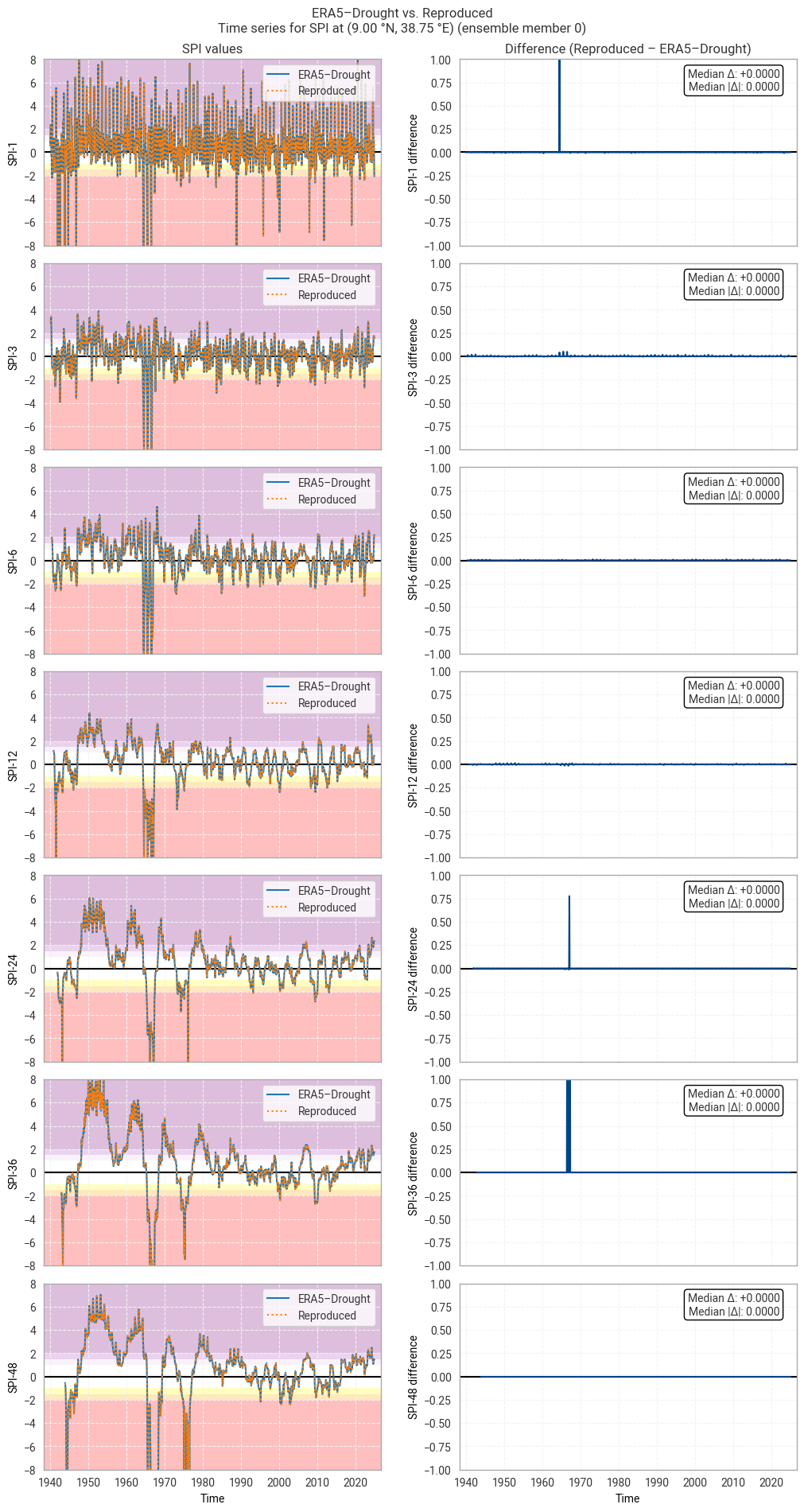
Fig. 6.1.17 SPI time series downloaded from ERA5–Drought and reproduced from ERA5 precipitation data (left) and the difference between the two (right), for the example site of Addis Ababa, Ethiopia. Colours in the left-hand column correspond to SPI categories (e.g. “extremely dry”) in [Keune+25]. This panel shows one member of the ensemble in either dataset.

Member 1

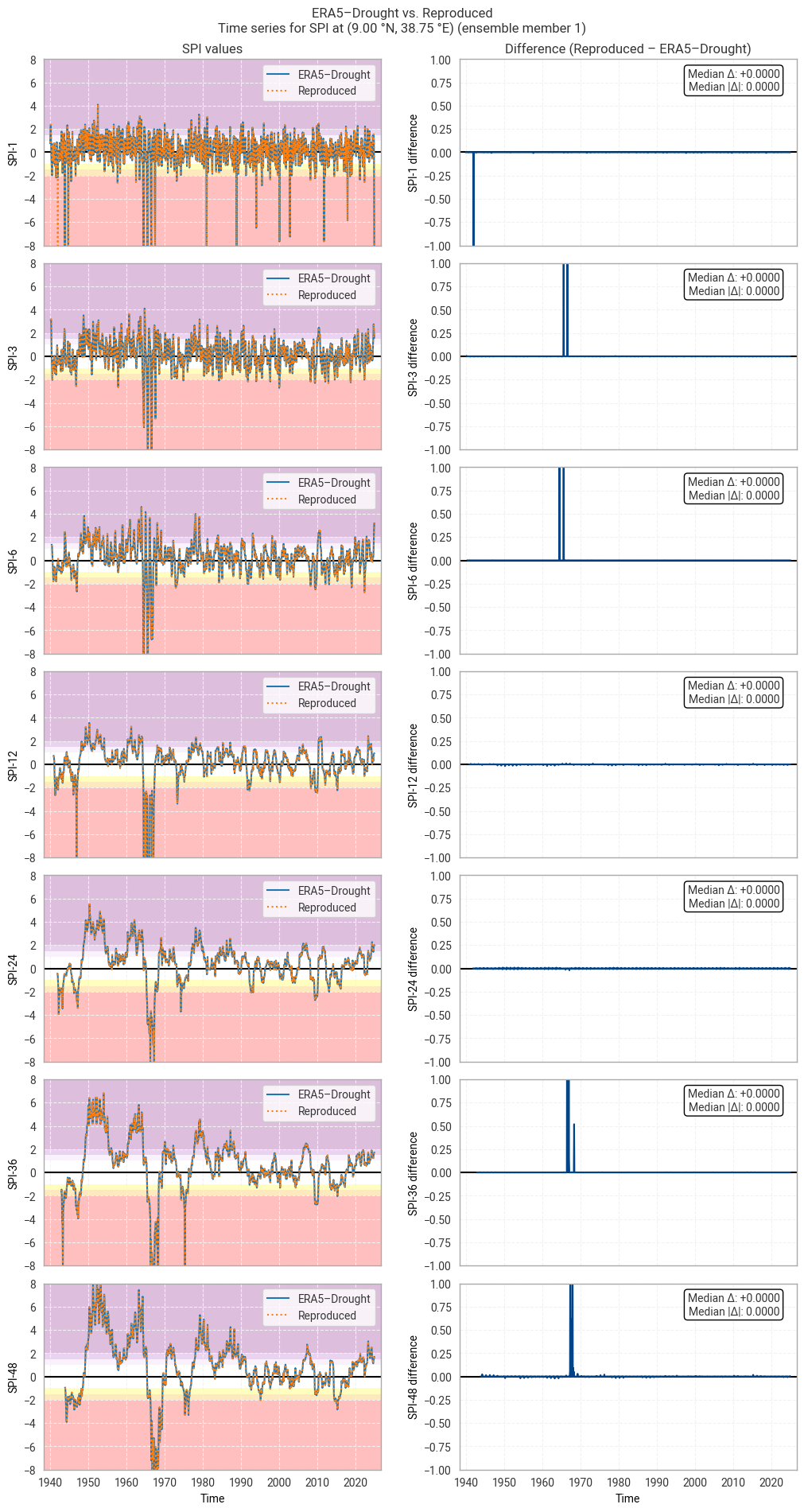
Fig. 6.1.18 SPI time series downloaded from ERA5–Drought and reproduced from ERA5 precipitation data (left) and the difference between the two (right), for the example site of Addis Ababa, Ethiopia. Colours in the left-hand column correspond to SPI categories (e.g. “extremely dry”) in [Keune+25]. This panel shows one member of the ensemble in either dataset.

Member 2

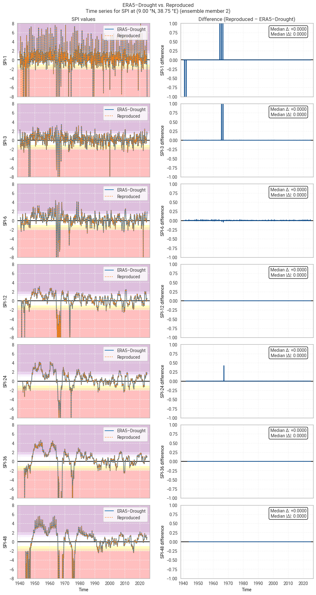
Fig. 6.1.19 SPI time series downloaded from ERA5–Drought and reproduced from ERA5 precipitation data (left) and the difference between the two (right), for the example site of Addis Ababa, Ethiopia. Colours in the left-hand column correspond to SPI categories (e.g. “extremely dry”) in [Keune+25]. This panel shows one member of the ensemble in either dataset.

Member 3

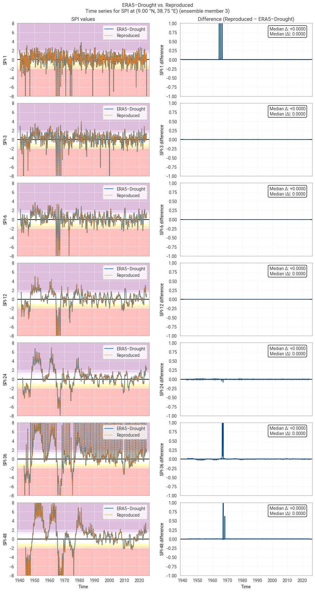
Fig. 6.1.20 SPI time series downloaded from ERA5–Drought and reproduced from ERA5 precipitation data (left) and the difference between the two (right), for the example site of Addis Ababa, Ethiopia. Colours in the left-hand column correspond to SPI categories (e.g. “extremely dry”) in [Keune+25]. This panel shows one member of the ensemble in either dataset.

Member 4

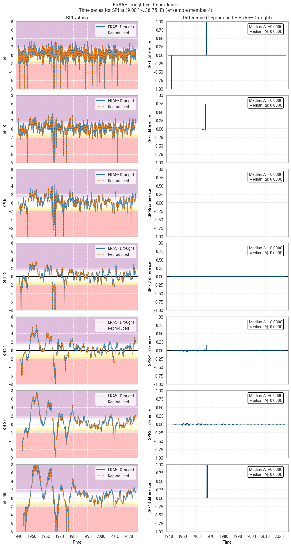
Fig. 6.1.21 SPI time series downloaded from ERA5–Drought and reproduced from ERA5 precipitation data (left) and the difference between the two (right), for the example site of Addis Ababa, Ethiopia. Colours in the left-hand column correspond to SPI categories (e.g. “extremely dry”) in [Keune+25]. This panel shows one member of the ensemble in either dataset.

Member 5

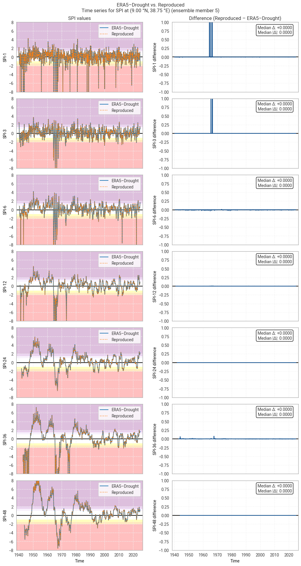
Fig. 6.1.22 SPI time series downloaded from ERA5–Drought and reproduced from ERA5 precipitation data (left) and the difference between the two (right), for the example site of Addis Ababa, Ethiopia. Colours in the left-hand column correspond to SPI categories (e.g. “extremely dry”) in [Keune+25]. This panel shows one member of the ensemble in either dataset.

Member 6

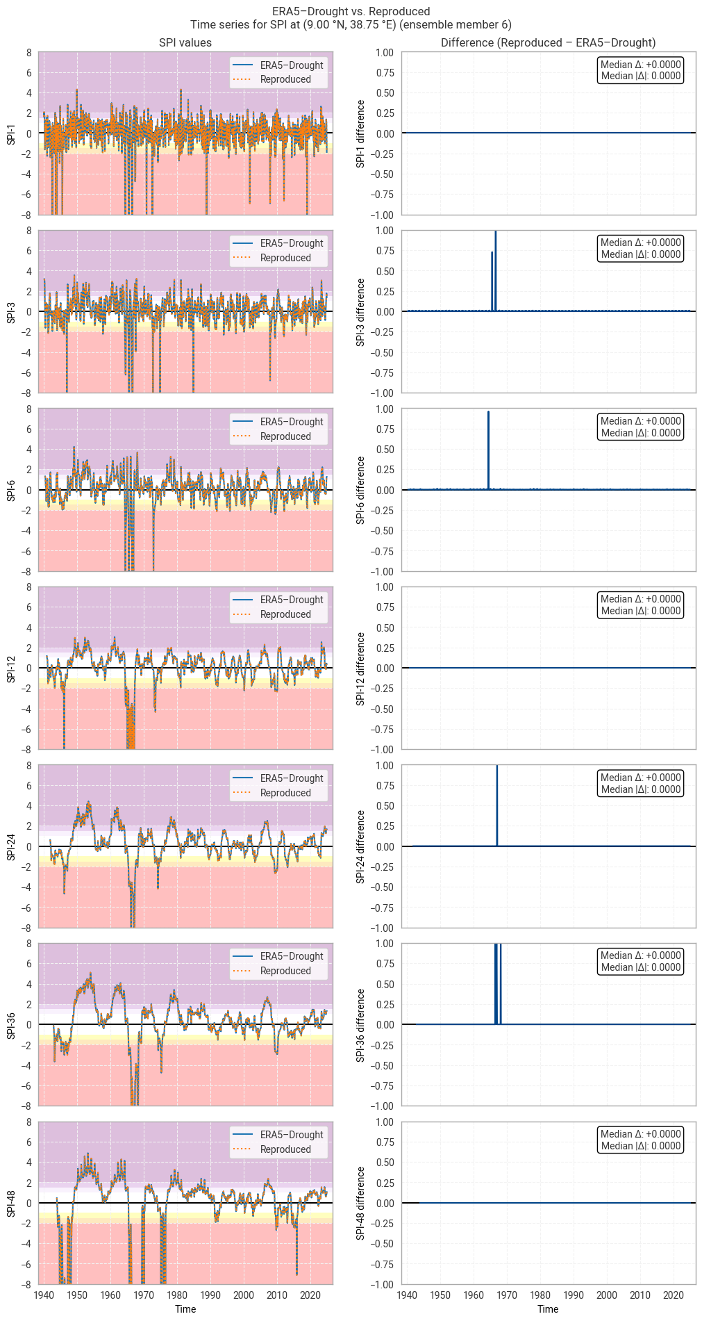
Fig. 6.1.23 SPI time series downloaded from ERA5–Drought and reproduced from ERA5 precipitation data (left) and the difference between the two (right), for the example site of Addis Ababa, Ethiopia. Colours in the left-hand column correspond to SPI categories (e.g. “extremely dry”) in [Keune+25]. This panel shows one member of the ensemble in either dataset.

Member 7

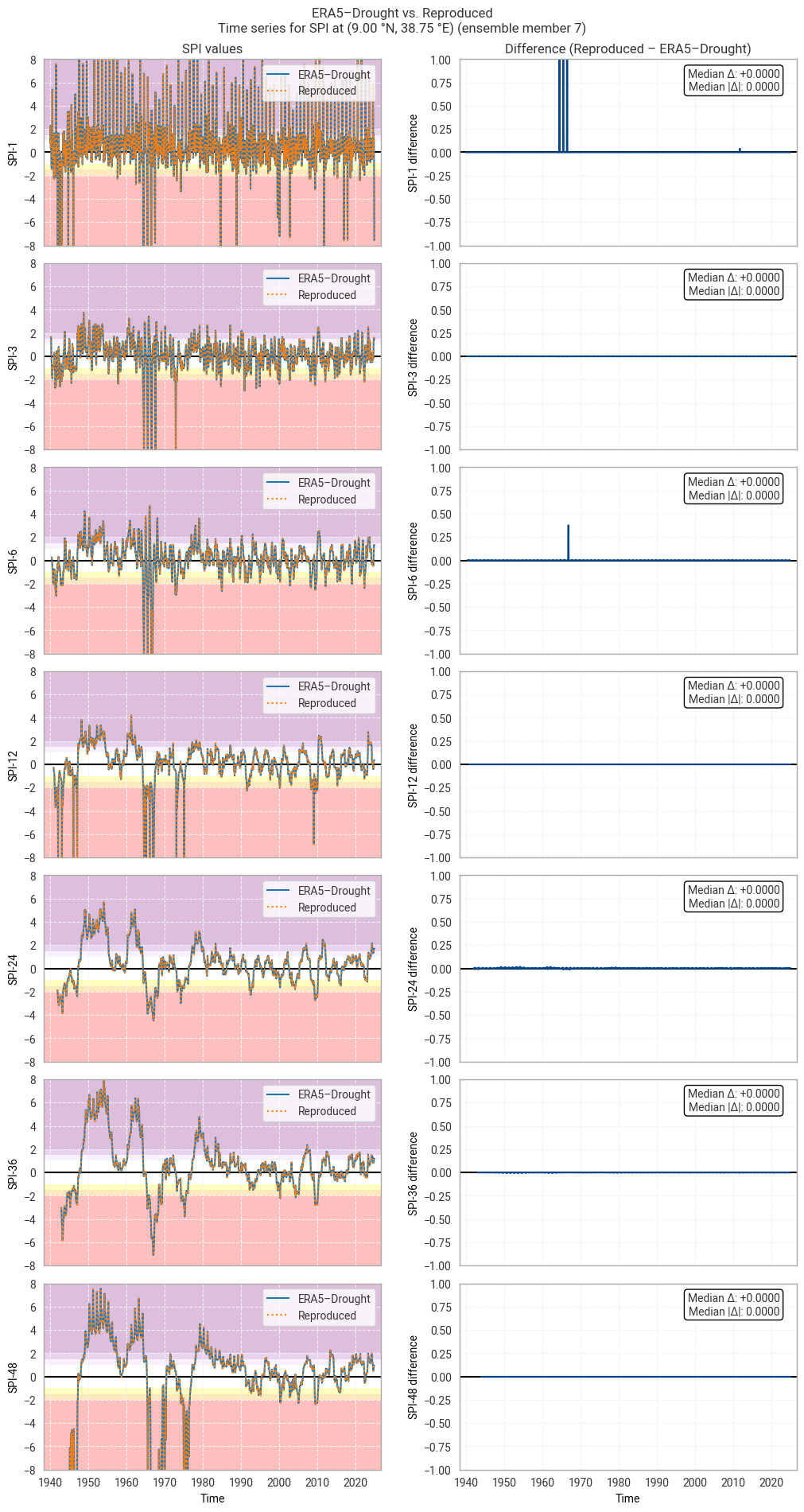
Fig. 6.1.24 SPI time series downloaded from ERA5–Drought and reproduced from ERA5 precipitation data (left) and the difference between the two (right), for the example site of Addis Ababa, Ethiopia. Colours in the left-hand column correspond to SPI categories (e.g. “extremely dry”) in [Keune+25]. This panel shows one member of the ensemble in either dataset.

Member 8

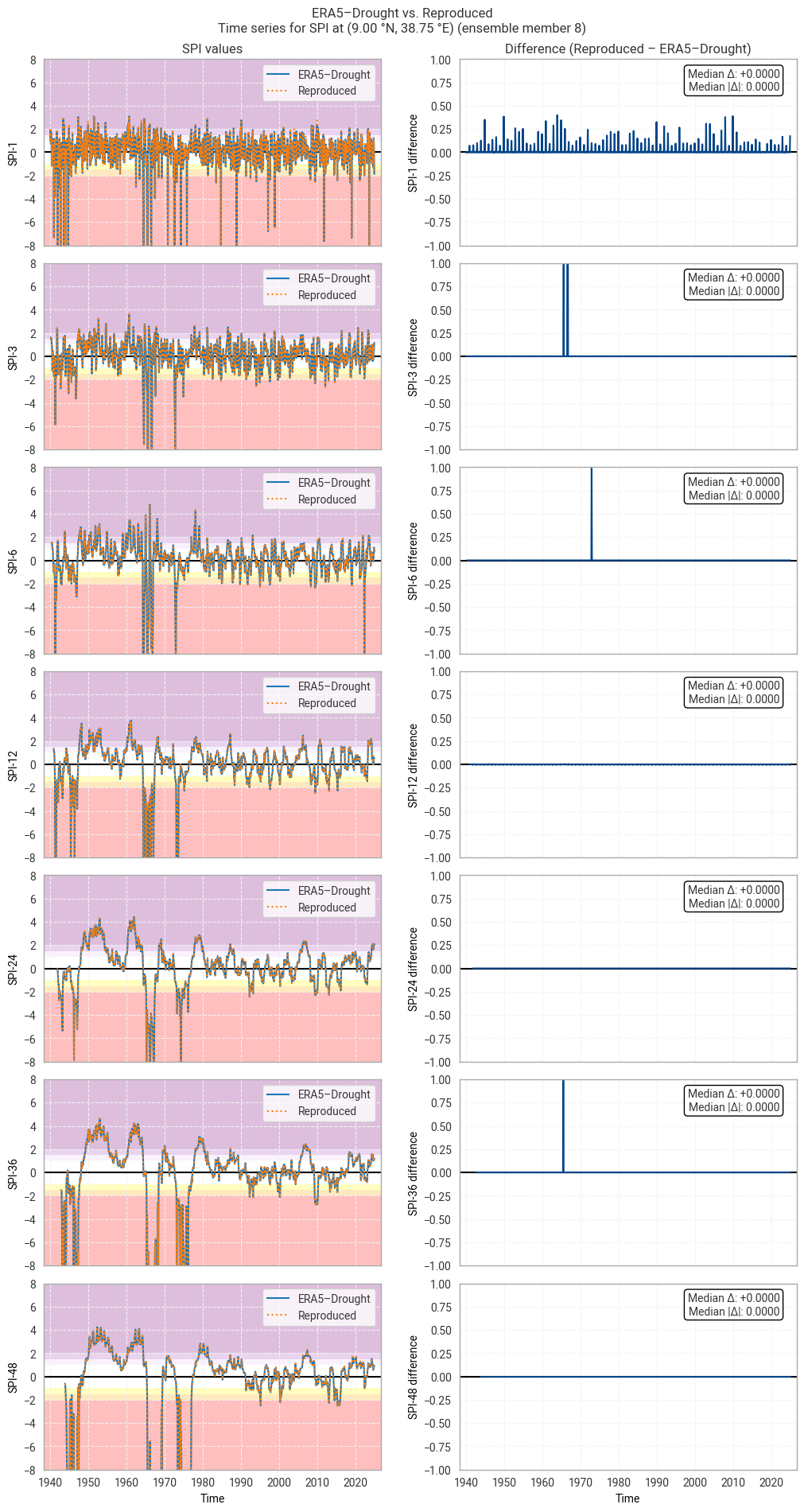
Fig. 6.1.25 SPI time series downloaded from ERA5–Drought and reproduced from ERA5 precipitation data (left) and the difference between the two (right), for the example site of Addis Ababa, Ethiopia. Colours in the left-hand column correspond to SPI categories (e.g. “extremely dry”) in [Keune+25]. This panel shows one member of the ensemble in either dataset.

Member 9

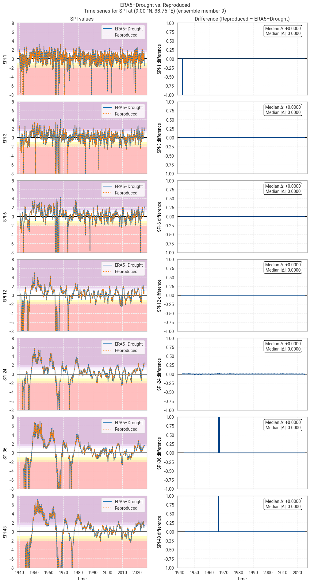
Fig. 6.1.26 SPI time series downloaded from ERA5–Drought and reproduced from ERA5 precipitation data (left) and the difference between the two (right), for the example site of Addis Ababa, Ethiopia. Colours in the left-hand column correspond to SPI categories (e.g. “extremely dry”) in [Keune+25]. This panel shows one member of the ensemble in either dataset.

Show code cell source

Hide code cell source

for m in trange(10):  # trange: range with tqdm progress bar
    plot_time_series_comparison_spei(spei_era5drought_site_ensemble.sel(number=m),
                                     spei_reproduced_site_ensemble.sel(number=m),
                                     title_suffix=f" at {label_site} (ensemble member {m})",
                                     glue_label=f"indicator_derived-drought-historical-monthly_consistency_q01_fig-spei-timeseries_ens_{m}")

Member 0

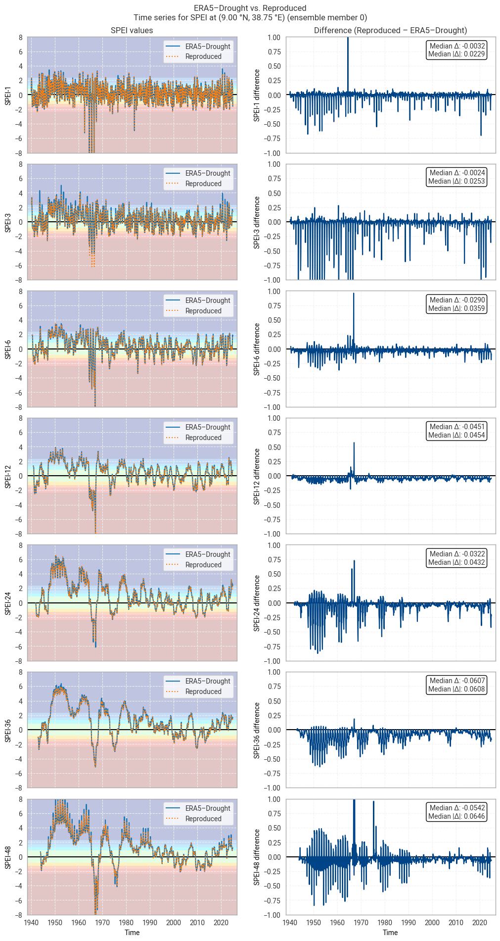
Fig. 6.1.27 SPEI time series downloaded from ERA5–Drought and reproduced from ERA5 precipitation data (left) and the difference between the two (right), for the example site of Addis Ababa, Ethiopia. Colours in the left-hand column correspond to SPEI categories (e.g. “extremely dry”) in [Keune+25]. This panel shows one member of the ensemble in either dataset.

Member 1

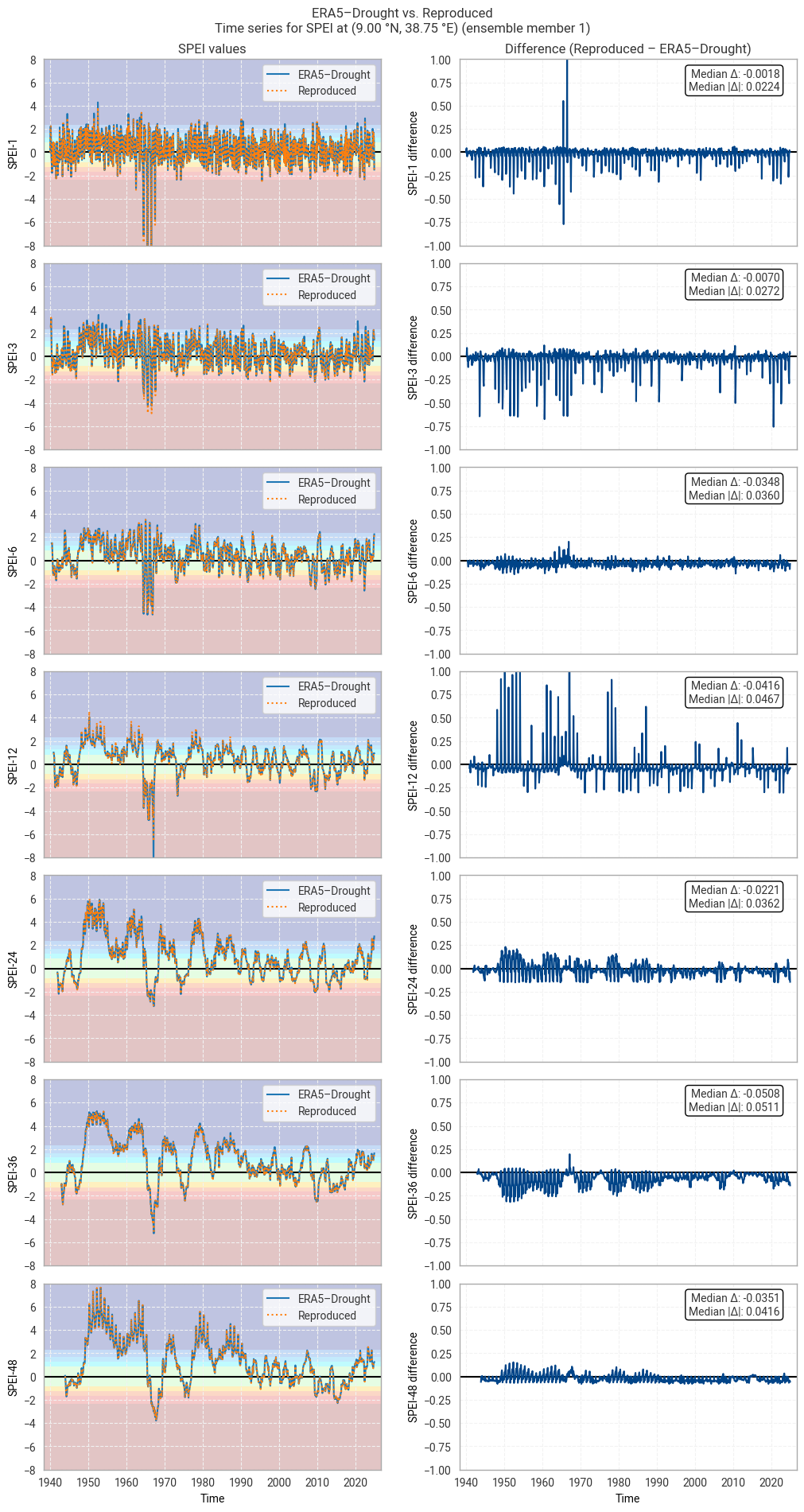
Fig. 6.1.28 SPEI time series downloaded from ERA5–Drought and reproduced from ERA5 precipitation data (left) and the difference between the two (right), for the example site of Addis Ababa, Ethiopia. Colours in the left-hand column correspond to SPEI categories (e.g. “extremely dry”) in [Keune+25]. This panel shows one member of the ensemble in either dataset.

Member 2

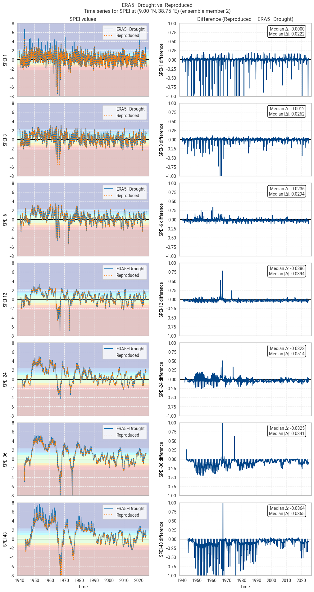
Fig. 6.1.29 SPEI time series downloaded from ERA5–Drought and reproduced from ERA5 precipitation data (left) and the difference between the two (right), for the example site of Addis Ababa, Ethiopia. Colours in the left-hand column correspond to SPEI categories (e.g. “extremely dry”) in [Keune+25]. This panel shows one member of the ensemble in either dataset.

Member 3

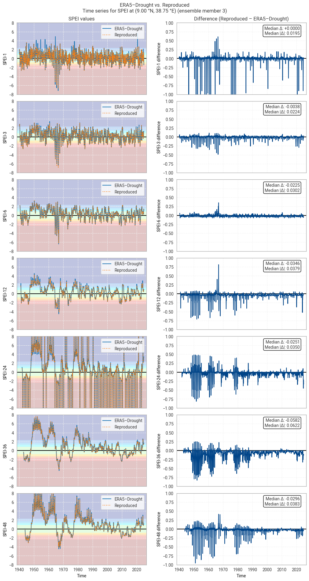
Fig. 6.1.30 SPEI time series downloaded from ERA5–Drought and reproduced from ERA5 precipitation data (left) and the difference between the two (right), for the example site of Addis Ababa, Ethiopia. Colours in the left-hand column correspond to SPEI categories (e.g. “extremely dry”) in [Keune+25]. This panel shows one member of the ensemble in either dataset.

Member 4

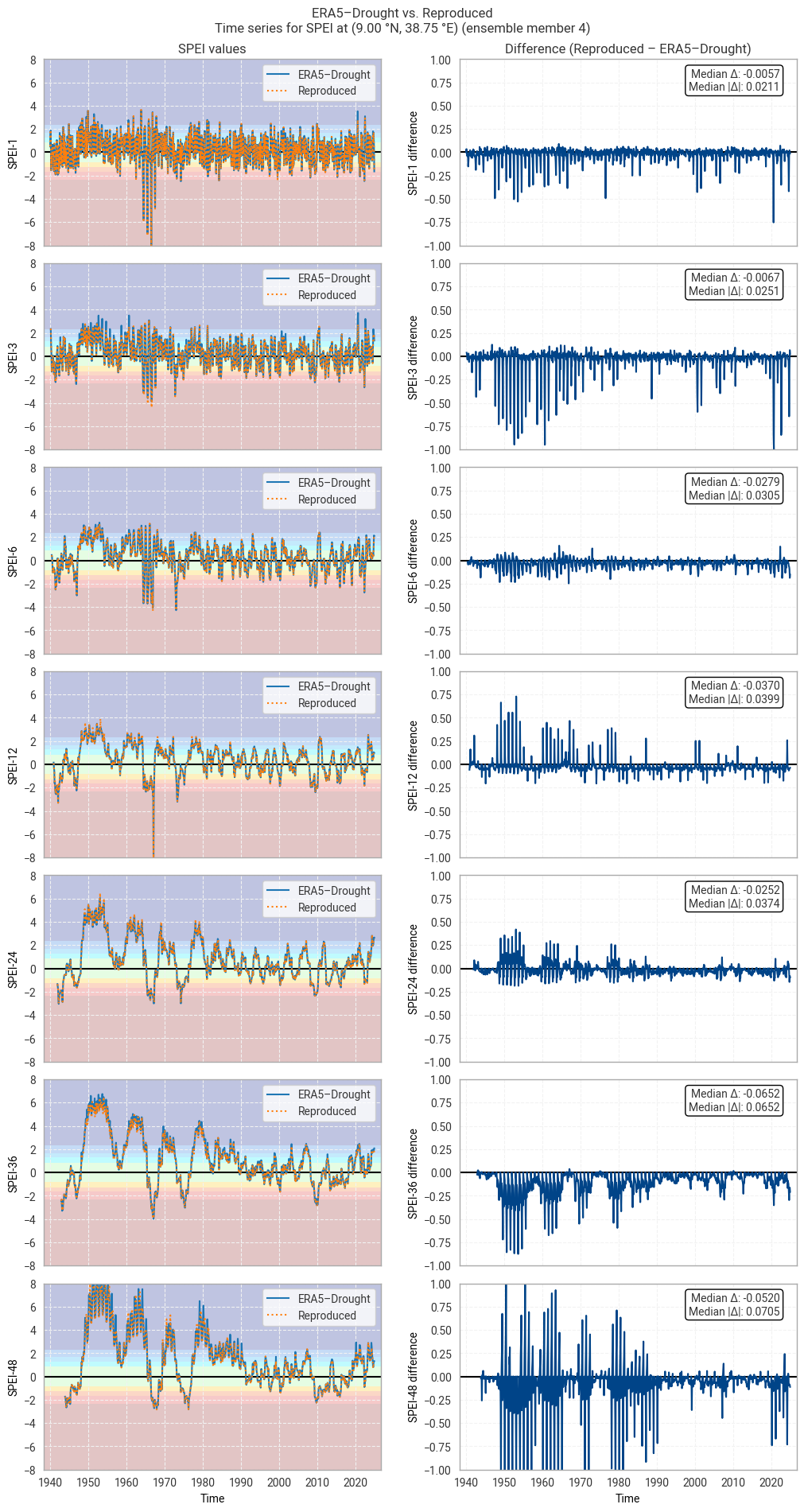
Fig. 6.1.31 SPEI time series downloaded from ERA5–Drought and reproduced from ERA5 precipitation data (left) and the difference between the two (right), for the example site of Addis Ababa, Ethiopia. Colours in the left-hand column correspond to SPEI categories (e.g. “extremely dry”) in [Keune+25]. This panel shows one member of the ensemble in either dataset.

Member 5

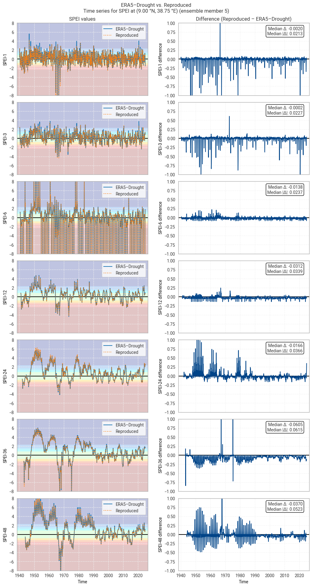
Fig. 6.1.32 SPEI time series downloaded from ERA5–Drought and reproduced from ERA5 precipitation data (left) and the difference between the two (right), for the example site of Addis Ababa, Ethiopia. Colours in the left-hand column correspond to SPEI categories (e.g. “extremely dry”) in [Keune+25]. This panel shows one member of the ensemble in either dataset.

Member 6

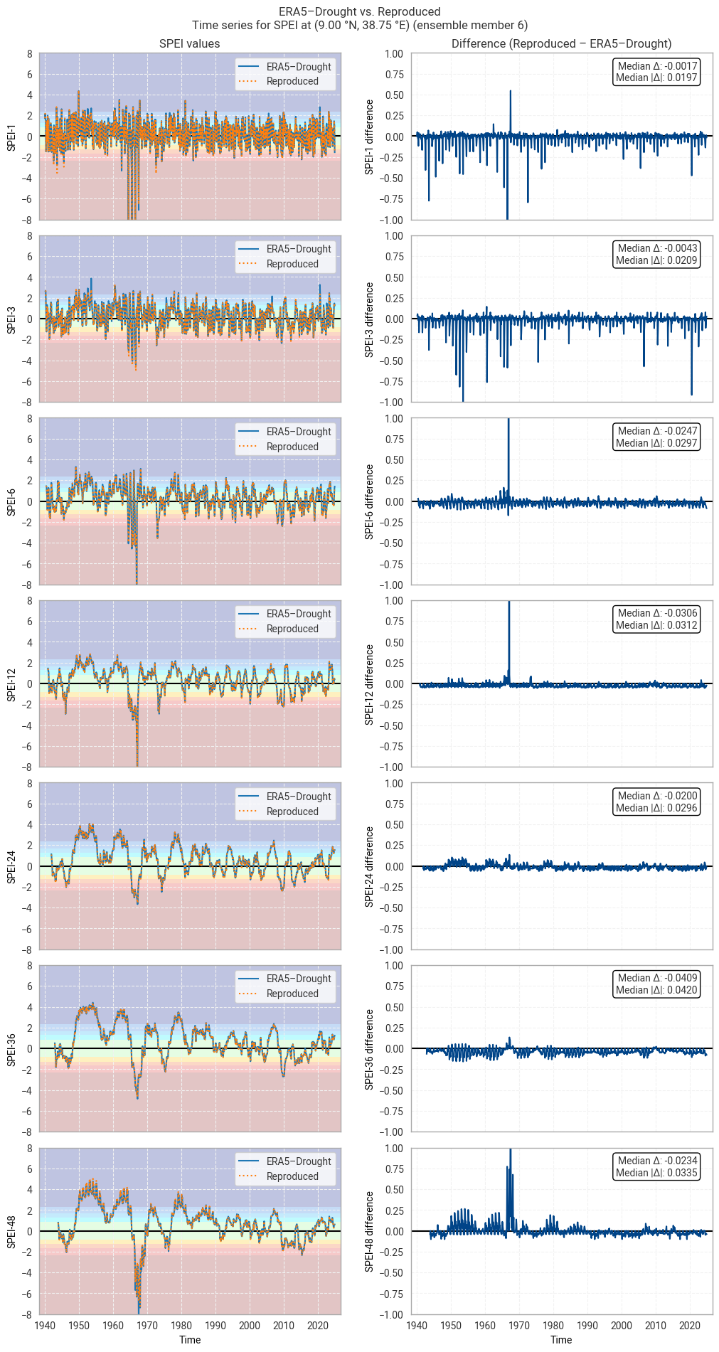
Fig. 6.1.33 SPEI time series downloaded from ERA5–Drought and reproduced from ERA5 precipitation data (left) and the difference between the two (right), for the example site of Addis Ababa, Ethiopia. Colours in the left-hand column correspond to SPEI categories (e.g. “extremely dry”) in [Keune+25]. This panel shows one member of the ensemble in either dataset.

Member 7

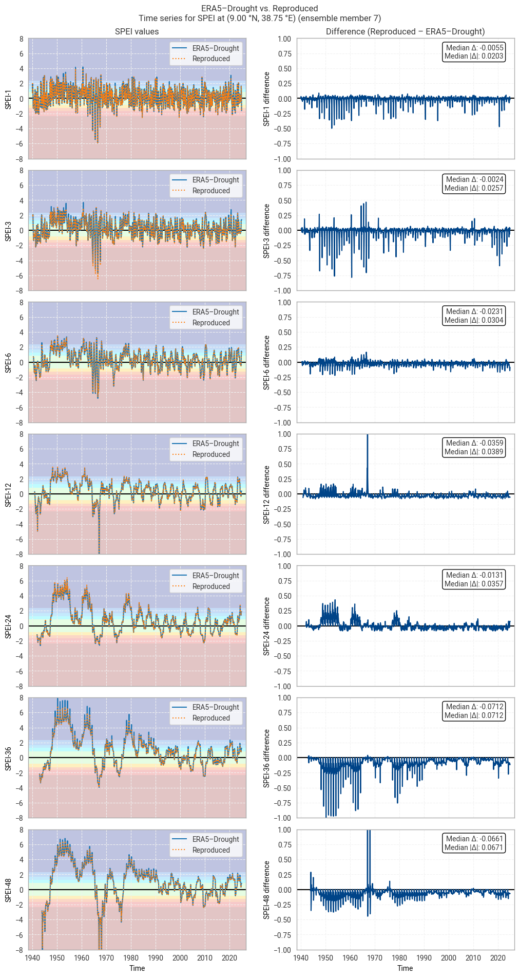
Fig. 6.1.34 SPEI time series downloaded from ERA5–Drought and reproduced from ERA5 precipitation data (left) and the difference between the two (right), for the example site of Addis Ababa, Ethiopia. Colours in the left-hand column correspond to SPEI categories (e.g. “extremely dry”) in [Keune+25]. This panel shows one member of the ensemble in either dataset.

Member 8

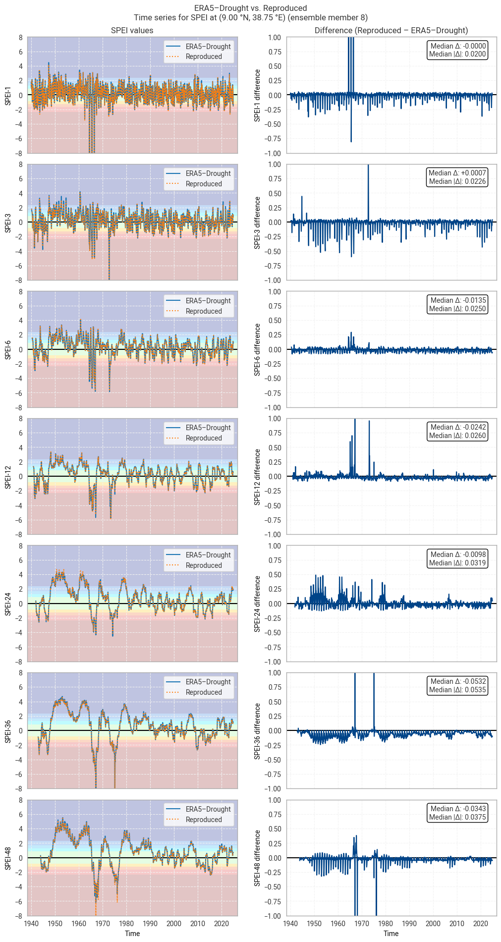
Fig. 6.1.35 SPEI time series downloaded from ERA5–Drought and reproduced from ERA5 precipitation data (left) and the difference between the two (right), for the example site of Addis Ababa, Ethiopia. Colours in the left-hand column correspond to SPEI categories (e.g. “extremely dry”) in [Keune+25]. This panel shows one member of the ensemble in either dataset.

Member 9

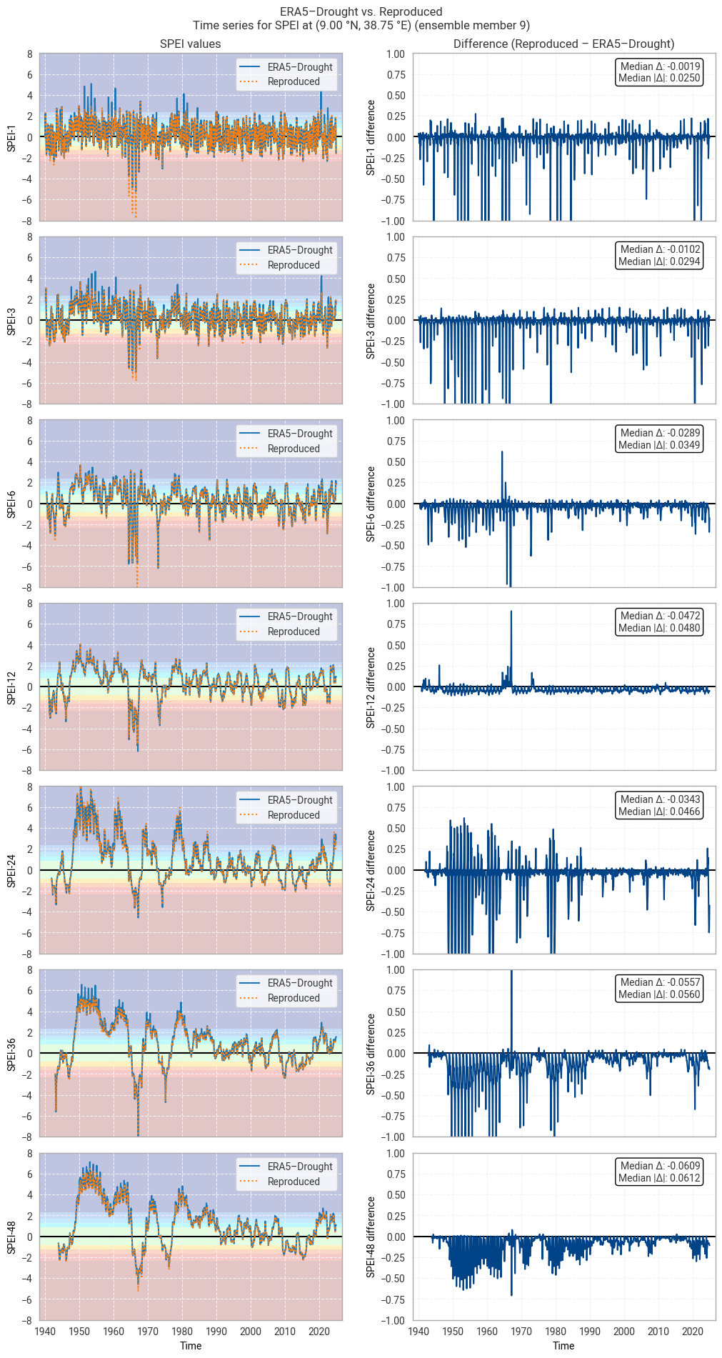
Fig. 6.1.36 SPEI time series downloaded from ERA5–Drought and reproduced from ERA5 precipitation data (left) and the difference between the two (right), for the example site of Addis Ababa, Ethiopia. Colours in the left-hand column correspond to SPEI categories (e.g. “extremely dry”) in [Keune+25]. This panel shows one member of the ensemble in either dataset.

6. Conclusions

In this notebook, we have assessed the reproducibility of drought indicators and associated quality flags in ERA5–Drought based on the underpinning ERA5 data. A pipeline for reproducing SPI and SPEI from ERA5 data was set up and applied to both the main reanalysis and the ensemble. Comparisons were made in one example site (Addis Ababa in Ethiopia) and the surrounding region (Horn of Africa); this notebook can easily be downloaded and adapted to a different area or time span of interest.

We can conclude that ERA5–Drought is highly reproducible. For SPI, reproduced values were generally identical to values in ERA5–Drought, with discrepancies taking the form of isolated spikes or occurring in areas that would be quality-masked anyway. The same was true for the probability of zero precipitation (p₀) quality flag, which matched in ≥99% of match-ups. Larger differences were seen in the SPI normality (α) quality flag (≥74% agreement) for reasons that are not entirely clear but likely related to zero-precipitation months that are captured by the p₀ quality flag. For SPEI, differences were larger, which may be explained by differences in the processing pipeline such as the exact choice of general logistic distribution used, but still small and unlikely to impact common use cases for drought classification and monitoring. The SPEI normality (α) quality flag showed good agreement (≥87%), especially considering the differences in the fitted distributions.

Users who intend to use ERA5–Drought can do so confidently. The included quality flags can be used to filter out low-quality data. Some of the effects seen in this notebook, such as slight differences in fitted parameters, are an inherent source of uncertainty in indicators like SPI and SPEI in any dataset. For a deeper exploration of the uncertainty in ERA5–Drought based on the included ensemble, we refer the reader to a forthcoming assessment on this subject.

ℹ️ If you want to know more

Key resources

The CDS catalogue entries for the data used were:

• Complete ERA5 global atmospheric reanalysis: reanalysis-era5-complete

• ERA5 hourly data on single levels from 1940 to present: reanalysis-era5-single-levels

• Monthly drought indices from 1940 to present derived from ERA5 reanalysis: derived-drought-historical-monthly

Code libraries used:

• earthkit

  • earthkit-data

  • earthkit-plots

• scipy.stats

More about drought indicators:

• SPI: The relationship of drought frequency and duration to time scales

• SPEI: A Multiscalar Drought Index Sensitive to Global Warming: The Standardized Precipitation Evapotranspiration Index

• Candidate Distributions for Climatological Drought Indices (SPI and SPEI)

• ERA5–Drought: Global drought indices based on ECMWF reanalysis

• The European and Global Drought Observatories (EDO, GDO)

More about ERA5:

• The ERA5 global reanalysis

• The ERA5 global reanalysis from 1940 to 2022

• Ensemble of data assimilations at ECMWF

References

[ECIU+25] Energy & Climate Intelligence Unit, ‘Estimated financial losses faced by UK farmers due dry weather impacts on key arable crops’, Energy & Climate Intelligence Unit, London, United Kingdom, Dec. 2025.

[IPCC+23] IPCC, ‘Climate Change 2023: Synthesis Report. Contribution of Working Groups I, II and III to the Sixth Assessment Report of the Intergovernmental Panel on Climate Change’, Intergovernmental Panel on Climate Change (IPCC), Geneva, Switzerland, Jul. 2023. doi: 10.59327/IPCC/AR6-9789291691647.

[UNICEF+24] UNICEF, ‘Latin America and Caribbean Region Flash Update No. 2 (Climate-related crisis in the Amazon Region)’, UNICEF, Nov. 2024.

[Franch-Pardo+25] I. Franch-Pardo, P. A. F. Puig, and A. Cerdà, ‘Geospatial Technologies in Crisis Response: Analyzing the 2024 Floods in Valencia, Spain’, European Journal of Geography, vol. 16, no. 2, pp. 286–297, Aug. 2025, doi: 10.48088/ejg.i.fra.16.2.286.297.

[McKee+93] T. B. McKee, N. J. Doesken, and J. Kleist, ‘The relationship of drought frequency and duration to time scales’, in Eighth Conference on Applied Climatology, Anaheim, California, USA, Jan. 1993.

[Keune+25] J. Keune, F. Di Giuseppe, C. Barnard, E. Damasio da Costa, and F. Wetterhall, ‘ERA5–Drought: Global drought indices based on ECMWF reanalysis’, Scientific Data, vol. 12, p. 616, Apr. 2025, doi: 10.1038/s41597-025-04896-y.

[EDO+25] EDO – European Drought Observatory, ‘EDO and GDO indicator factsheet: Standardized Precipitation Index (SPI)’, Copernicus Emergency Management Service, Mar. 2025. Accessed: Feb. 09, 2026. [Online]. Available: https://drought.emergency.copernicus.eu/data/factsheets/factsheet_spi.pdf

[Vicente-Serrano+10] S. M. Vicente-Serrano, S. Beguería, and J. I. López-Moreno, ‘A Multiscalar Drought Index Sensitive to Global Warming: The Standardized Precipitation Evapotranspiration Index’, Journal of Climate, vol. 23, no. 7, pp. 1696–1718, Apr. 2010, doi: 10.1175/2009JCLI2909.1.

[Soci+24] C. Soci et al., ‘The ERA5 global reanalysis from 1940 to 2022’, Quarterly Journal of the Royal Meteorological Society, vol. 150, no. 764, pp. 4014–4048, Jul. 2024, doi: 10.1002/qj.4803.

[Hersbach+20] H. Hersbach et al., ‘The ERA5 global reanalysis’, Quarterly Journal of the Royal Meteorological Society, vol. 146, no. 730, pp. 1999–2049, May 2020, doi: 10.1002/qj.3803.

[Stagge+15] J. H. Stagge, L. M. Tallaksen, L. Gudmundsson, A. F. Van Loon, and K. Stahl, ‘Candidate Distributions for Climatological Drought Indices (SPI and SPEI)’, International Journal of Climatology, vol. 35, no. 13, pp. 4027–4040, Feb. 2015, doi: 10.1002/joc.4267.

[Gebrechorkos+19] S. H. Gebrechorkos, S. Hülsmann, and C. Bernhofer, ‘Long-term trends in rainfall and temperature using high-resolution climate datasets in East Africa’, Sci Rep, vol. 9, no. 1, p. 11376, Aug. 2019, doi: 10.1038/s41598-019-47933-8.

[Shapiro+65] S. S. Shapiro and M. B. Wilk, ‘An analysis of variance test for normality (complete samples)’, Biometrika, vol. 52, no. 3–4, pp. 591–611, Dec. 1965, doi: 10.1093/biomet/52.3-4.591.