CMIP6 Climate Projections: evaluating bias in extreme temperature indices for the reinsurance sector.

CMIP6 Climate Projections: evaluating bias in extreme temperature indices for the reinsurance sector.#

Use case: Defining a strategy to optimise reinsurance protections#

Quality assessment question#

How well do CMIP6 projections represent climatology and trends of air temperature extremes in Europe?

Production date: 23-05-2024

Produced by: CMCC foundation - Euro-Mediterranean Center on Climate Change. Albert Martinez Boti.

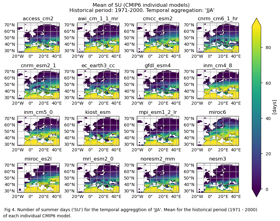
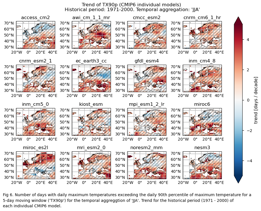
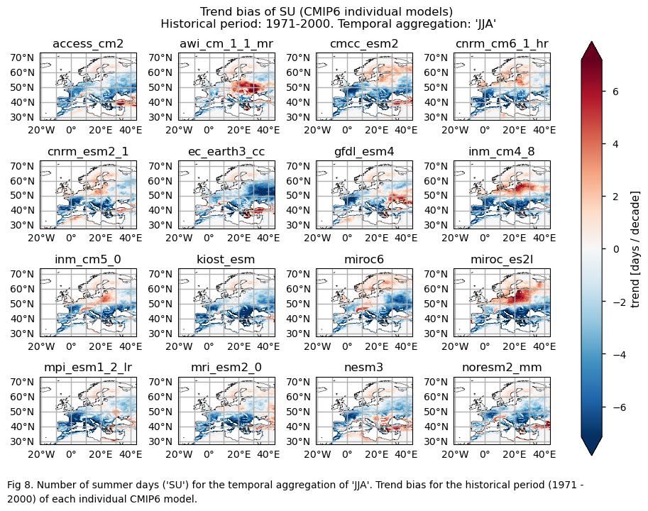
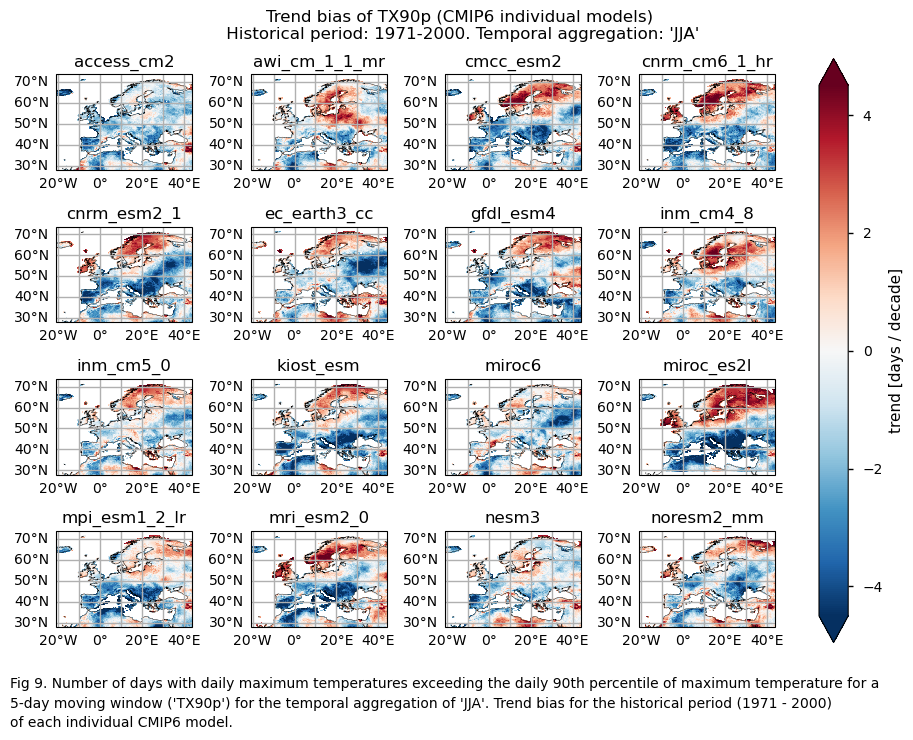
Climate change has a major impact on the reinsurance market [1][2]. In the third assessment report of the IPCC, hot temperature extremes were already presented as relevant to insurance and related services [3]. Consequently, the need for reliable regional and global climate projections has become paramount, offering valuable insights for optimising reinsurance strategies in the face of a changing climate landscape. Nonetheless, despite their pivotal role, uncertainties inherent in these projections can potentially lead to misuse [4][5]. This underscores the importance of accurately calculating and accounting for uncertainties to ensure their appropriate consideration. This notebook utilises data from a subset of models from CMIP6 Global Climate Models (GCMs) and compares them with ERA5 reanalysis, serving as the reference product. Two maximum-temperature-based indices from ECA&D indices (one of physical nature and the other of statistical nature) are computed using the icclim Python package. The first index, identified by the ETCCDI short name ‘SU’, quantifies the occurrence of summer days (i.e., with daily maximum temperatures exceeding 25°C) within a year or a season (JJA in this notebook). The second index, labeled ‘TX90p’, describes the number of days with daily maximum temperatures exceeding the daily 90th percentile of maximum temperature for a 5-day moving window. Within this notebook, these calculations are performed over the historical period spanning from 1971 to 2000. It is important to mention that the results presented here pertain to a specific subset of the CMIP6 ensemble and may not be generalisable to the entire dataset. Also note that a separate assessment examines the representation of trends of these indices for the same models during a fixed future period (2015-2099), while another assessment looks at the projected climate signal of these indices for the same models at a 2°C Global Warming Level.

Quality assessment statement#

CMIP6 projections based on maximum temperature indices can be valuable for designing strategies to optimise reinsurance protections. However, it is crucial for users to acknowledge that all climate projections inherently contain certain biases. This is especially significant when using projections in regions with complex orography or extensive continental areas, where biases are more pronounced and impact the accuracy of the projections. Therefore, users should exercise caution and consider these limitations when applying the projections to their specific use cases, understanding that biases in the mean climate and trends affect indices differently and that the choice of bias correction method should be tailored accordingly [6][7].
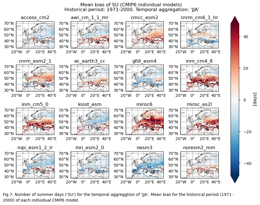
GCMs exhibit biases in capturing mean values of extreme temperature indices like the number of summer days (‘SU’) and days exceeding the 90th percentile threshold (‘TX90p’), with underestimation of index magnitudes, especially in continental areas and regions with complex terrain.
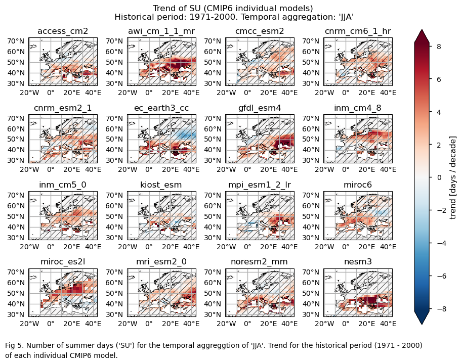
ERA5 shows that the magnitude of the historical trend varies spatially. The trend bias assessment suggests that, overall, the trend derived from the CMIP6 projections is underestimated with slight overestimations observed in certain regions. Hence, users need to consider this regional variation in both the trend and its bias.
Despite limitations and biases, the considered subset of CMIP6 models generally reproduces historical trends reasonably well for the summer season (JJA), providing a foundation for understanding past climate behavior. These findings also increase confidence (though they do not ensure accuracy) when analysing future trends using these models.

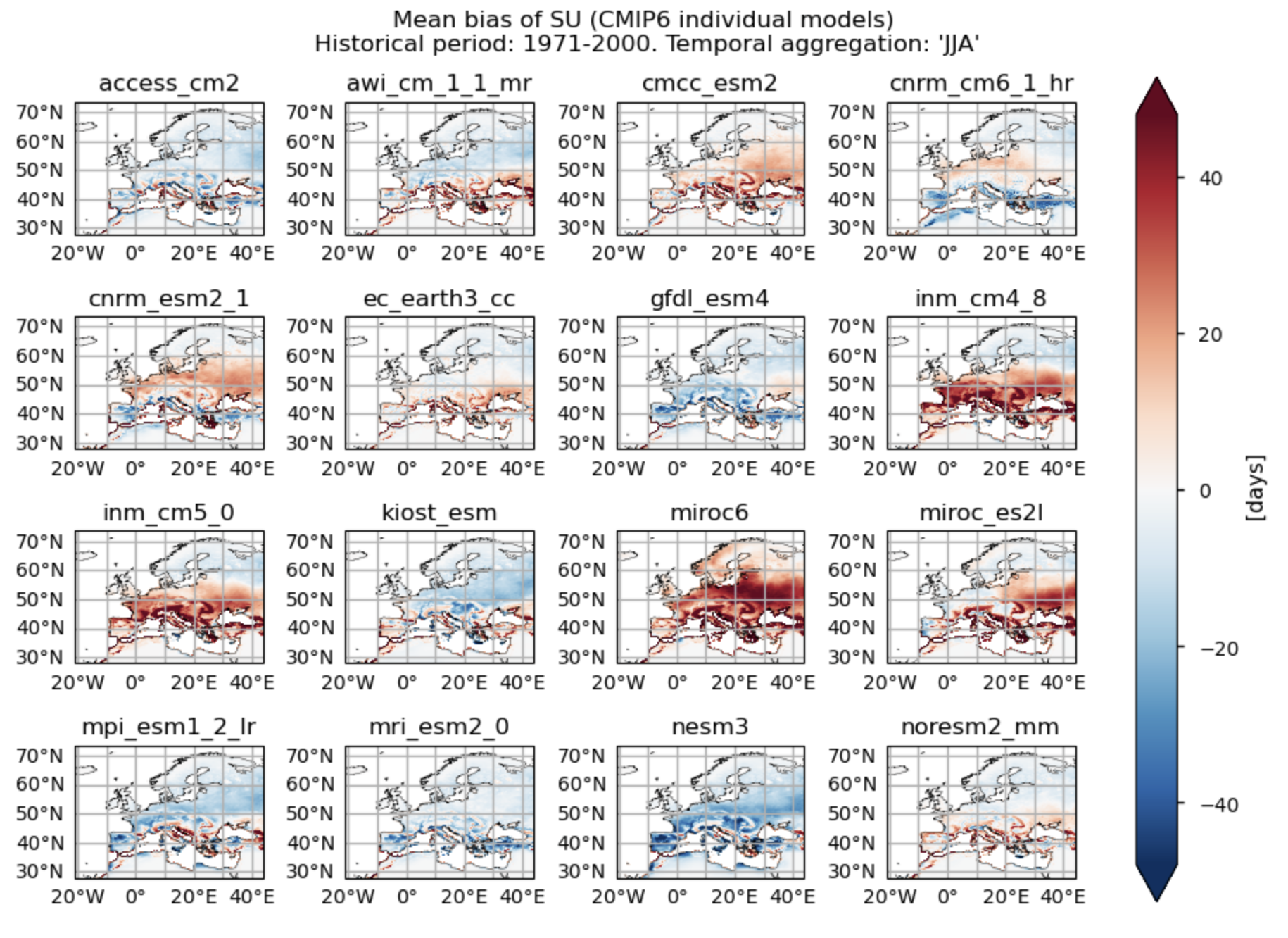
Fig A. Number of summer days ('SU') for the temporal aggregation of 'JJA'. Mean bias for the historical period (1971 - 2000) of each individual CMIP6 model.

Methodology#

This notebook provides an assessment of the systematic errors (trend and climate mean) in a subset of 16 models from CMIP6. It achieves this by comparing the model predictions with the ERA5 reanalysis for the maximum-temperature-based indices of ‘SU’ and ‘TX90p’, calculated over the temporal aggregation of JJA and for the historical period spanning from 1971 to 2000 (chosen to allow comparison to CORDEX models in another assessment). In particular, spatial patterns of climate mean and trend, along with biases, are examined and displayed for each model and the ensemble median (calculated for each grid cell). Additionally, spatially-averaged trend values are analysed and presented using box plots to provide an overview of trend behavior across the distribution of the chosen subset of models when averaged across Europe.

The analysis and results follow the next outline:

1. Parameters, requests and functions definition

1.1. Import packages
1.2. Define Parameters
1.3. Define models
1.4. Define ERA5 request
1.5. Define model requests
1.6. Functions to cache

2. Downloading and processing

2.1. Download and transform ERA5
2.2. Download and transform models
2.3. Apply land-sea mask, change attributes and cut the region to show

3. Plot and describe results

3.1. Define plotting functions
3.2. Plot ensemble maps
3.3. Plot model maps
3.4. Plot bias maps
3.5. Boxplots of the historical trend
3.6. Results summary and discussion

Analysis and results#

1. Parameters, requests and functions definition#

1.1. Import packages#

1.2. Define Parameters#

In the “Define Parameters” section, various customisable options for the notebook are specified:

The initial and ending year used for the historical period can be specified by changing the parameters year_start and year_stop (1971-2000 is chosen for consistency between CMIP6 and CORDEX).
The timeseries set the temporal aggregation. For instance, selecting “JJA” implies considering only the JJA season.
collection_id provides the choice between Global Climate Models CMIP6 or Regional Climate Models CORDEX. Although the code allows choosing between CMIP6 or CORDEX, the example provided in this notebook deals with CMIP6.
area allows specifying the geographical domain of interest.
The interpolation_method parameter allows selecting the interpolation method when regridding is performed over the indices.
The chunk selection allows the user to define if dividing into chunks when downloading the data on their local machine. Although it does not significantly affect the analysis, it is recommended to keep the default value for optimal performance.

1.3. Define models#

The following climate analyses are performed considering a subset of GCMs from CMIP6. Models names are listed in the parameters below. Some variable-dependent parameters are also selected, as the index_names parameter, which specifies the temperature-based indices (‘SU’ and ‘TX90p’ in our case) from the icclim Python package.

The selected CMIP6 models have available both the historical and SSP5-8.5 experiments.

Show code cell source Hide code cell source

match variable:
    case "temperature":
        resample_reduction = "max"
        index_names = ("SU", "TX90p")
        era5_variable = "2m_temperature"
        cmip6_variable = "daily_maximum_near_surface_air_temperature"
        cordex_variable = "maximum_2m_temperature_in_the_last_24_hours"
        models_cmip6 = (
            "access_cm2",
            "awi_cm_1_1_mr",
            "cmcc_esm2",
            "cnrm_cm6_1_hr",
            "cnrm_esm2_1",
            "ec_earth3_cc",
            "gfdl_esm4",
            "inm_cm4_8",
            "inm_cm5_0",
            "kiost_esm",
            "mpi_esm1_2_lr",
            "miroc6",
            "miroc_es2l", 
            "mri_esm2_0",
            "noresm2_mm",
            "nesm3",    
        )   
        cbars = {"cmap_divergent": "RdBu_r", "cmap_sequential": "viridis"}
        #Define dictionaries to use in titles and caption
        long_name = {
            "SU":"Number of summer days",
            "TX90p":"Number of days with daily maximum temperatures exceeding the daily 90th percentile of maximum temperature for a 5-day moving window",
        }
    case "precipitation":
        resample_reduction = "sum"
        index_names = ("CWD", "R20mm", "RR1", "RX1day", "RX5day")
        era5_variable = "total_precipitation"
        cmip6_variable = "precipitation"
        cordex_variable = "mean_precipitation_flux"
        models_cmip6 = (
            "access_cm2",
            "bcc_csm2_mr",
            "cmcc_esm2",
            "cnrm_cm6_1_hr",
            "cnrm_esm2_1",
            "ec_earth3_cc",
            "gfdl_esm4",
            "inm_cm4_8",
            "inm_cm5_0",
            "mpi_esm1_2_lr",
            "miroc6",
            "miroc_es2l", 
            "mri_esm2_0",
            "noresm2_mm",
            "nesm3",
            "ukesm1_0_ll",
        )
        cbars = {"cmap_divergent": "RdBu", "cmap_sequential": "viridis_r"}
        #Define dictionaries to use in titles and caption
        long_name = {
            "RX1day": "Maximum 1-day total precipitation",
            "RX5day": "Maximum 5-day total precipitation",
            "RR1":"Number of wet days (Precip >= 1mm)",
            "R20mm":"Number of heavy precipitation days (Precip >= 20mm)",
            "CWD":"Maximum consecutive wet days",
        }
    case _:
        raise NotImplementedError(f"{variable=}")

models_cordex = (
    "clmcom_clm_cclm4_8_17",
    "clmcom_eth_cosmo_crclim",
    "cnrm_aladin63",
    "dmi_hirham5",
    "knmi_racmo22e",
    "mohc_hadrem3_ga7_05",
    "mpi_csc_remo2009",
    "smhi_rca4",
    "uhoh_wrf361h",
)

1.4. Define ERA5 request#

Within this notebook, ERA5 serves as the reference product. In this section, we set the required parameters for the cds-api data-request of ERA5.

1.5. Define model requests#

In this section we set the required parameters for the cds-api data-request.

When Weights = True, spatial weighting is applied for calculations requiring spatial data aggregation. This is particularly relevant for CMIP6 GCMs with regular lon-lat grids that do not consider varying surface extensions at different latitudes. In contrast, CORDEX RCMs, using rotated grids, inherently account for different cell surfaces based on latitude, eliminating the need for a latitude cosine multiplicative factor (Weights = False).

Show code cell source Hide code cell source

request_cmip6 = {
    "format": "zip",
    "temporal_resolution": "daily",
    "experiment": "historical",
    "variable": cmip6_variable,
    "year": [
        str(year) for year in range(year_start - 1, year_stop + 1)
    ],  # Include D(year-1)
    "month": [f"{month:02d}" for month in range(1, 13)],
    "day": [f"{day:02d}" for day in range(1, 32)],
    "area": area,
}

request_cordex = {
    "format": "zip",
    "domain": "europe",
    "experiment": "historical",
    "horizontal_resolution": "0_11_degree_x_0_11_degree",
    "temporal_resolution": "daily_mean",
    "variable": cordex_variable,
    "gcm_model": "mpi_m_mpi_esm_lr",
    "ensemble_member": "r1i1p1",
}


def get_cordex_years(
    year_start,
    year_stop,
    timeseries,
    start_years=list(range(1951, 2097, 5)),
    end_years=list(range(1955, 2101, 5)),
):
    start_year = []
    end_year = []
    years = set(range(year_start - int(timeseries == "DJF"), year_stop + 1))
    for start, end in zip(start_years, end_years):
        if years & set(range(start, end + 1)):
            start_year.append(start)
            end_year.append(end)
    return start_year, end_year


model_requests = {}
if collection_id == "CORDEX":
    for model in models_cordex:
        start_years = [1970 if model in ("smhi_rca4", "uhoh_wrf361h") else 1966] + list(
            range(1971, 2097, 5)
        )
        end_years = [1970] + list(range(1975, 2101, 5))
        model_requests[model] = (
            "projections-cordex-domains-single-levels",
            [
                {
                    "rcm_model": model,
                    **request_cordex,
                    "start_year": start_year,
                    "end_year": end_year,
                }
                for start_year, end_year in zip(
                    *get_cordex_years(
                        year_start,
                        year_stop,
                        timeseries,
                        start_years=start_years,
                        end_years=end_years,
                    )
                )
            ],
        )
elif collection_id == "CMIP6":
    for model in models_cmip6:
        model_requests[model] = (
            "projections-cmip6",
            download.split_request(request_cmip6 | {"model": model}, chunks=chunks),
        )
else:
    raise ValueError(f"{collection_id=}")

1.6. Functions to cache#

In this section, functions that will be executed in the caching phase are defined. Caching is the process of storing copies of files in a temporary storage location, so that they can be accessed more quickly. This process also checks if the user has already downloaded a file, avoiding redundant downloads.

Functions description:

The select_timeseries function subsets the dataset based on the chosen timeseries parameter.
The compute_indices function utilises the icclim package to calculate the selected maximum-temperature-based indices.
The compute_trends function employs the Mann-Kendall test for trend calculation.
Finally, the compute_indices_and_trends function selects the temporal aggregation using the select_timeseries function. It then computes daily maximum temperature (only if we are dealing with ERA5), calculates maximum-temperature-based indices via the compute_indices function, determines the indices mean over the historical period (1971-2000), obtain the trends using the compute_trends function, and offers an option for regridding to ERA5 if required.

Show code cell source Hide code cell source

def select_timeseries(ds, timeseries, year_start, year_stop, index_names):
    if timeseries == "annual":
        return ds.sel(time=slice(str(year_start), str(year_stop)))
    ds=ds.sel(time=slice(f"{year_start-1}-12", f"{year_stop}-11"))
    if "RX5day" in index_names:
        return ds
    return ds.where(ds["time"].dt.season == timeseries, drop=True)  
    
def compute_indices(ds, index_names, timeseries, tmpdir):
    labels, datasets = zip(*ds.groupby("time.year"))
    paths = [f"{tmpdir}/{label}.nc" for label in labels]
    datasets = [ds.chunk(-1) for ds in datasets]
    xr.save_mfdataset(datasets, paths)

    ds = xr.open_mfdataset(paths)
    in_files = f"{tmpdir}/rechunked.zarr"
    chunks = {dim: -1 if dim == "time" else "auto" for dim in ds.dims}
    ds.chunk(chunks).to_zarr(in_files)

    datasets = [
        icclim.index(
            index_name=index_name,
            in_files=in_files,
            out_file=f"{tmpdir}/{index_name}.nc",
            slice_mode="year" if timeseries == "annual" else timeseries,
        )
        for index_name in index_names
    ]

    return xr.merge(datasets).drop_dims("bounds")


def compute_trends(ds):
    datasets = []
    (lat,) = set(ds.dims) & set(ds.cf.axes["Y"])
    (lon,) = set(ds.dims) & set(ds.cf.axes["X"])
    coords_name = {
        "time": "time",
        "y": lat,
        "x": lon,
    }
    for index, da in ds.data_vars.items():
        ds = Mann_Kendall_test(
            da - da.mean("time"),
            alpha=0.05,
            method="theilslopes",
            coords_name=coords_name,
        ).compute()
        ds = ds.rename({k: v for k, v in coords_name.items() if k in ds.dims})
        ds = ds.assign_coords({dim: da[dim] for dim in ds.dims})
        datasets.append(ds.expand_dims(index=[index]))
    ds = xr.concat(datasets, "index")
    return ds


def add_bounds(ds):
    for coord in {"latitude", "longitude"} - set(ds.cf.bounds):
        ds = ds.cf.add_bounds(coord)
    return ds


def get_grid_out(request_grid_out, method):
    ds_regrid = download.download_and_transform(*request_grid_out)
    coords = ["latitude", "longitude"]
    if method == "conservative":
        ds_regrid = add_bounds(ds_regrid)
        for coord in list(coords):
            coords.extend(ds_regrid.cf.bounds[coord])
    grid_out = ds_regrid[coords]
    coords_to_drop = set(grid_out.coords) - set(coords) - set(grid_out.dims)
    grid_out = ds_regrid[coords].reset_coords(coords_to_drop, drop=True)
    grid_out.attrs = {}
    return grid_out


def compute_indices_and_trends(
    ds,
    index_names,
    timeseries,
    year_start,
    year_stop,
    resample_reduction=None,
    request_grid_out=None,
    **regrid_kwargs,
):
    assert (request_grid_out and regrid_kwargs) or not (
        request_grid_out or regrid_kwargs
    )
    ds = ds.drop_vars([var for var, da in ds.data_vars.items() if len(da.dims) != 3])
    ds = ds[list(ds.data_vars)]

    # Original bounds for conservative interpolation
    if regrid_kwargs.get("method") == "conservative":
        ds = add_bounds(ds)
        bounds = [
            ds.cf.get_bounds(coord).reset_coords(drop=True)
            for coord in ("latitude", "longitude")
        ]
    else:
        bounds = []

    ds = select_timeseries(ds, timeseries, year_start, year_stop,index_names)
    if resample_reduction:
        resampled = ds.resample(time="1D")
        ds = getattr(resampled, resample_reduction)(keep_attrs=True)
        if resample_reduction == "sum":
            for da in ds.data_vars.values():
                da.attrs["units"] = f"{da.attrs['units']} / day"
    with tempfile.TemporaryDirectory() as tmpdir:
        ds_indices = compute_indices(ds, index_names, timeseries, tmpdir).compute()
        ds_trends = compute_trends(ds_indices)
        ds = ds_indices.mean("time", keep_attrs=True)
        ds = ds.merge(ds_trends)
        if request_grid_out:
            ds = diagnostics.regrid(
                ds.merge({da.name: da for da in bounds}),
                grid_out=get_grid_out(request_grid_out, regrid_kwargs["method"]),
                **regrid_kwargs,
            )
        return ds

2. Downloading and processing#

2.1. Download and transform ERA5#

In this section, the download.download_and_transform function from the ‘c3s_eqc_automatic_quality_control’ package is employed to download ERA5 reference data, select the temporal aggregation (“JJA” in our example), compute daily maximum temperature from hourly data, compute the maximum-temperature-based indices, calculate the mean and trend for the historical period (1971-2000) and cache the result (to avoid redundant downloads and processing).

2.2. Download and transform models#

In this section, the download.download_and_transform function from the ‘c3s_eqc_automatic_quality_control’ package is employed to download daily data from the CMIP6 models, compute the maximum-temperature-based indices for the selected temporal aggregation, calculate the mean and trend over the historical period (1971-2000), interpolate to ERA5’s grid (only for the cases in which it is specified, in the other cases, the original model’s grid is mantained), and cache the result (to avoid redundant downloads and processing).

model='access_cm2'
model='awi_cm_1_1_mr'
model='cmcc_esm2'
model='cnrm_cm6_1_hr'
model='cnrm_esm2_1'
model='ec_earth3_cc'
model='gfdl_esm4'
model='inm_cm4_8'
model='inm_cm5_0'
model='kiost_esm'
model='mpi_esm1_2_lr'
model='miroc6'
model='miroc_es2l'
model='mri_esm2_0'
model='noresm2_mm'
model='nesm3'

2.3. Apply land-sea mask, change attributes and cut the region to show#

This section performs the following tasks:

Cut the region of interest.
Downloads the sea mask for ERA5.
Applies the sea mask to both ERA5 data and the model data, which were previously regridded to ERA5’s grid (i.e., it applies the ERA5 sea mask to ds_interpolated).
Regrids the ERA5 land-sea mask to the model’s grid and applies it to them.
Change some variable attributes for plotting purposes.

Note: ds_interpolated contains data from the models (mean and trend over the historical period, p-value of the trends…) regridded to ERA5. model_datasets contain the same data but in the original grid of each model.

3. Plot and describe results#

This section will display the following results:

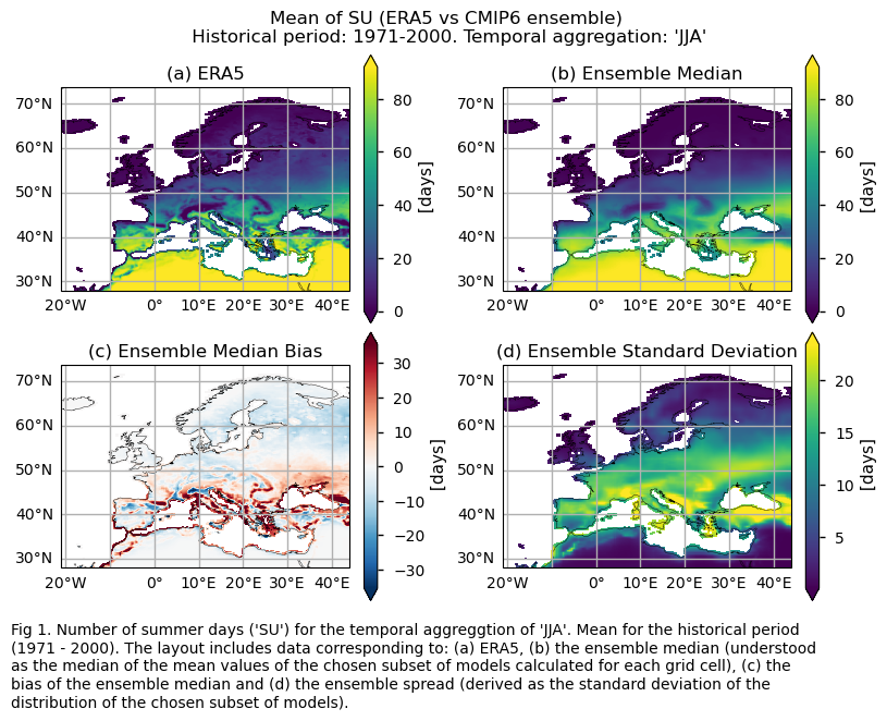
Maps representing the spatial distribution of the historical mean values (1971-2000) of the ‘SU’ index for ERA5, each model individually, the ensemble median (understood as the median of the mean values of the chosen subset of models calculated for each grid cell), and the ensemble spread (derived as the standard deviation of the distribution of the chosen subset of models).
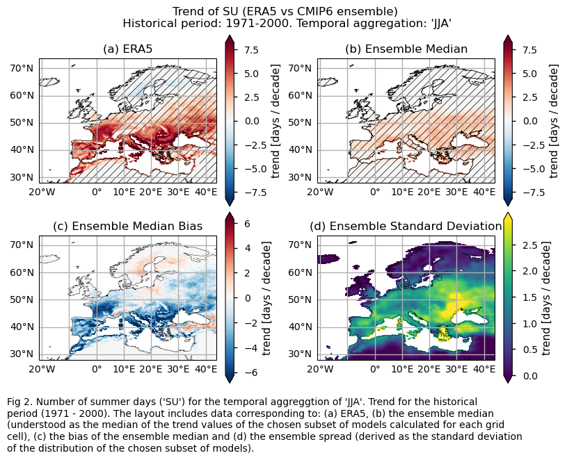
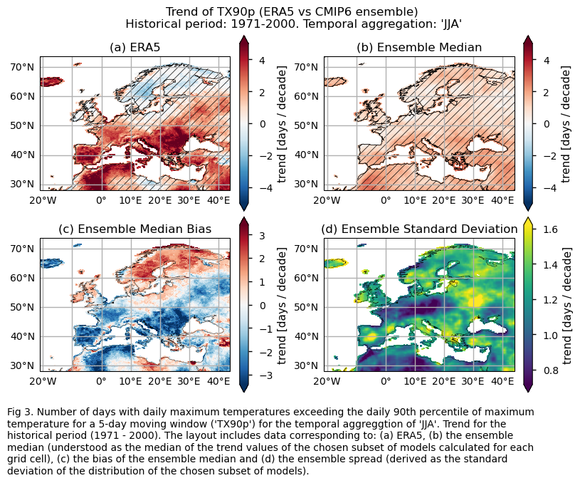
Maps representing the spatial distribution of the historical trends (1971-2000) of the indices ‘SU’ and ‘TX90p’. Similar to the first analysis, this includes ERA5, each model individually, the ensemble median (understood as the median of the trend values of the chosen subset of models calculated for each grid cell), and the ensemble spread (derived as the standard deviation of the distribution of the chosen subset of models).
Bias maps of the historical mean values.
Trend bias maps.
Boxplots representing statistical distributions (PDF) built on the spatially-averaged historical trends from each considered model, displayed together with ERA5.

3.1. Define plotting functions#

The functions presented here are used to plot the mean values and trends calculated over the historical period (1971-2000) for each of the indices (‘SU’ and ‘TX90p’).

For a selected index, three layout types can be displayed, depending on the chosen function:

Layout including the reference ERA5 product, the ensemble median, the bias of the ensemble median, and the ensemble spread: plot_ensemble() is used.
Layout including every model (for the trend and mean values): plot_models() is employed.
Layout including the bias of every model (for the trend and mean values): plot_models() is used again.

trend==True argument allows displaying trend values over the historical period, while trend==False will show mean values. When the trend argument is set to True, regions with no significance are hatched. For individual models and ERA5, a grid point is considered to have a statistically significant trend when the p-value is lower than 0.05 (in such cases, no hatching is shown). However, for determining trend significance for the ensemble median (understood as the median of the trend values of the chosen subset of models calculated for each grid cell), reliance is placed on agreement categories, following the advanced approach proposed in AR6 IPCC on pages 1945-1950. The hatch_p_value_ensemble() function is used to distinguish, for each grid point, between three possible cases:

If more than 66% of the models are statistically significant (p-value < 0.05) and more than 80% of the models share the same sign, we consider the ensemble median trend to be statistically significant, and there is agreement on the sign. To represent this, no hatching is used.
If less than 66% of the models are statistically significant, regardless of agreement on the sign of the trend, hatching is applied (indicating that the ensemble median trend is not statistically significant).
If more than 66% of the models are statistically significant but less than 80% of the models share the same sign, we consider the ensemble median trend to be statistically significant, but there is no agreement on the sign of the trend. This is represented using crosses.

Show code cell source Hide code cell source

#Define function to plot the caption of the figures (for the ensmble case)
def add_caption_ensemble(trend,exp):
    #Add caption to the figure
    match trend:
        case True:
            caption_text= (
                f"Fig {fig_number}. {long_name[index]} ('{index}') for "
                f"the temporal aggreggtion of '{timeseries}'. Trend for "
                f"the {exp} period ({year_start} - {year_stop}). The layout "
                f"includes data corresponding to: (a) ERA5, (b) the ensemble median "
                f"(understood as the median of the trend values of the chosen subset of models " 
                f"calculated for each grid cell), "
                f"(c) the bias of the ensemble median and (d) the ensemble spread "
                f"(derived as the standard deviation of the distribution of the chosen " 
                f"subset of models)."
            )
        case False:
            caption_text= (
                f"Fig {fig_number}. {long_name[index]} ('{index}') for "
                f"the temporal aggreggtion of '{timeseries}'. Mean for "
                f"the {exp} period ({year_start} - {year_stop}). The layout "
                f"includes data corresponding to: (a) ERA5, (b) the ensemble median "
                f"(understood as the median of the mean values of the chosen subset of models " 
                f"calculated for each grid cell), "
                f"(c) the bias of the ensemble median and (d) the ensemble spread "
                f"(derived as the standard deviation of the distribution of the chosen " 
                f"subset of models)."
            )
            
    wrapped_lines = textwrap.wrap(caption_text, width=105)
    # Add each line to the figure
    for i, line in enumerate(wrapped_lines):
        fig.text(0, -0.05  - i * 0.03, line, ha='left', fontsize=10)
    #end captioning


#Define function to plot the caption of the figures (for the individual models case)
def add_caption_models(trend,bias,exp):
    #Add caption to the figure
    if bias: 
        match trend:
            case True:
                caption_text = (
                    f"Fig {fig_number}. {long_name[index]} ('{index}') for the "
                    f"temporal aggregation of '{timeseries}'. Trend bias for the "
                    f"{exp} period ({year_start} - {year_stop}) of each individual "
                    f"{collection_id} model."
                )
            case False:
                caption_text = (
                    f"Fig {fig_number}. {long_name[index]} ('{index}') for the "
                    f"temporal aggreggtion of '{timeseries}'. Mean bias for the "
                    f"{exp} period ({year_start} - {year_stop}) of each individual "
                    f"{collection_id} model."
                )
    else:
        match trend:
            case True:
                caption_text = (
                    f"Fig {fig_number}. {long_name[index]} ('{index}') for the "
                    f"temporal aggreggtion of '{timeseries}'. Trend for the {exp} "
                    f"period ({year_start} - {year_stop}) of each individual "
                    f"{collection_id} model."
                ) 
            case False:
                caption_text = (
                    f" Fig {fig_number}. {long_name[index]} ('{index}') for the "
                    f"temporal aggreggtion of '{timeseries}'. Mean for the {exp} "
                    f"period ({year_start} - {year_stop}) of each individual "
                    f"{collection_id} model."
                )
    wrapped_lines = textwrap.wrap(caption_text, width=120)
    # Add each line to the figure
    for i, line in enumerate(wrapped_lines):
        fig.text(0, -0.05  - i * 0.03, line, ha='left', fontsize=10)





def hatch_p_value(da, ax, **kwargs):
    default_kwargs = {
        "plot_func": "contourf",
        "show_stats": False,
        "cmap": "none",
        "add_colorbar": False,
        "levels": [0, 0.05, 1],
        "hatches": ["", "/" * 3],
    }
    kwargs = default_kwargs | kwargs

    title = ax.get_title()
    plot_obj = plot.projected_map(da, ax=ax, **kwargs)
    ax.set_title(title)
    return plot_obj


def hatch_p_value_ensemble(trend, p_value, ax):
    n_models = trend.sizes["model"]
    robust_ratio = (p_value <= 0.05).sum("model") / n_models
    robust_ratio = robust_ratio.where(p_value.notnull().any("model"))
    signs = xr.concat([(trend > 0).sum("model"), (trend < 0).sum("model")], "sign")
    sign_ratio = signs.max("sign") / n_models
    robust_threshold = 0.66
    sign_ratio = sign_ratio.where(robust_ratio > robust_threshold)
    for da, threshold, character in zip(
        [robust_ratio, sign_ratio], [robust_threshold, 0.8], ["/", "\\"]
    ):
        hatch_p_value(da, ax=ax, levels=[0, threshold, 1], hatches=[character * 3, ""])


def set_extent(da, axs, area):
    extent = [area[i] for i in (1, 3, 2, 0)]
    for i, coord in enumerate(extent):
        extent[i] += -1 if i % 2 else +1
    for ax in axs:
        ax.set_extent(extent)


def plot_models(
    data,
    da_for_kwargs=None,
    p_values=None,
    col_wrap=4 if collection_id=="CMIP6" else 3,
    subplot_kw={"projection": ccrs.PlateCarree()},
    figsize=None,
    layout="constrained",
    area=area,
    flip_cmaps=False,
    **kwargs,
):
    if isinstance(data, dict):
        assert da_for_kwargs is not None
        model_dataarrays = data
    else:
        da_for_kwargs = da_for_kwargs or data
        model_dataarrays = dict(data.groupby("model"))

    if p_values is not None:
        model_p_dataarrays = (
            p_values if isinstance(p_values, dict) else dict(p_values.groupby("model"))
        )
    else:
        model_p_dataarrays = None

    # Get kwargs
    default_kwargs = {"robust": True, "extend": "both"}
    kwargs = default_kwargs | kwargs
    kwargs = xr.plot.utils._determine_cmap_params(da_for_kwargs.values, **kwargs)

    fig, axs = plt.subplots(
        *(col_wrap, math.ceil(len(model_dataarrays) / col_wrap)),
        subplot_kw=subplot_kw,
        figsize=figsize,
        layout=layout,
    )
    axs = axs.flatten()
    for (model, da), ax in zip(model_dataarrays.items(), axs):
        pcm = plot.projected_map(
            da, ax=ax, show_stats=False, add_colorbar=False, **kwargs
        )
        ax.set_title(model)
        if model_p_dataarrays is not None:
            hatch_p_value(model_p_dataarrays[model], ax)
    set_extent(da_for_kwargs, axs, area)
    fig.colorbar(
        pcm,
        ax=axs.flatten(),
        extend=kwargs["extend"],
        location="right",
        label=f"{da_for_kwargs.attrs.get('long_name', '')} [{da_for_kwargs.attrs.get('units', '')}]",
    )
    return fig


def plot_ensemble(
    da_models,
    da_era5=None,
    p_value_era5=None,
    p_value_models=None,
    subplot_kw={"projection": ccrs.PlateCarree()},
    figsize=None,
    layout="constrained",
    cbar_kwargs=None,
    area=area,
    flip_cmaps=False,
    **kwargs,
):
    # Get kwargs
    default_kwargs = {"robust": True, "extend": "both"}
    kwargs = default_kwargs | kwargs
    kwargs = xr.plot.utils._determine_cmap_params(
        da_models.values if da_era5 is None else da_era5.values, **kwargs
    )
    if da_era5 is None and cbar_kwargs is None:
        cbar_kwargs = {"orientation": "horizontal"}

    # Figure
    fig, axs = plt.subplots(
        *(1 if da_era5 is None else 2, 2),
        subplot_kw=subplot_kw,
        figsize=figsize,
        layout=layout,
    )
    axs = axs.flatten()
    axs_iter = iter(axs)

    # ERA5
    if da_era5 is not None:
        ax = next(axs_iter)
        plot.projected_map(
            da_era5, ax=ax, show_stats=False, cbar_kwargs=cbar_kwargs, **kwargs
        )
        if p_value_era5 is not None:
            hatch_p_value(p_value_era5, ax=ax)
        ax.set_title("(a) ERA5")

    # Median
    ax = next(axs_iter)
    median = da_models.median("model", keep_attrs=True)
    plot.projected_map(
        median, ax=ax, show_stats=False, cbar_kwargs=cbar_kwargs, **kwargs
    )
    if p_value_models is not None:
        hatch_p_value_ensemble(trend=da_models, p_value=p_value_models, ax=ax)
    ax.set_title("(b) Ensemble Median" if da_era5 is not None else "(a) Ensemble Median")

    # Bias
    if da_era5 is not None:
        ax = next(axs_iter)
        with xr.set_options(keep_attrs=True):
            bias = median - da_era5
        plot.projected_map(
            bias,
            ax=ax,
            show_stats=False,
            center=0,
            cbar_kwargs=cbar_kwargs,
            **default_kwargs,
        )
        ax.set_title("(c) Ensemble Median Bias")

    # Std
    ax = next(axs_iter)
    std = da_models.std("model", keep_attrs=True)
    plot.projected_map(
        std, ax=ax, show_stats=False, cbar_kwargs=cbar_kwargs, **default_kwargs
    )
    ax.set_title("(d) Ensemble Standard Deviation" if da_era5 is not None else "(b) Ensemble Standard Deviation")

    set_extent(da_models, axs, area)
    return fig

3.2. Plot ensemble maps#

In this section, we invoke the plot_ensemble() function to visualise the mean values and trends calculated over the historical period (1971-2000) for the model ensemble and ERA5 reference product across Europe. Note that the model data used in this section has previously been interpolated to the ERA5 grid.

Specifically, for each of the indices (‘SU’ and ‘TX90p’), this section presents two layouts:

Only for the ‘SU’ index: mean values of the historical period (1971-2000) for: (a) the reference ERA5 product, (b) the ensemble median (understood as the median of the mean values of the chosen subset of models calculated for each grid cell), (c) the bias of the ensemble median, and (d) the ensemble spread (derived as the standard deviation of the distribution of the chosen subset of models).
Trend values of the historical period (1971-2000) for: (a) the reference ERA5 product, (b) the ensemble median (understood as the median of the trend values of the chosen subset of models calculated for each grid cell), (c) the bias of the ensemble median, and (d) the ensemble spread (derived as the standard deviation of the distribution of the chosen subset of models).

../_images/f5bcd4abaa236df4e7c23c292a2b67614ad58c447d15d2213e7a3f150d503af1.png

../_images/29b3d3ddd4480ded9a07f9d7aff9ba0b2a4ce963f2e9578ae433f9c2356b9c3e.png

../_images/7c6a826be225559d97887f4530787a4ea66ff6cbce0e700928557b4cedc37717.png

3.3. Plot model maps#

In this section, we invoke the plot_models() function to visualise the mean values and trends calculated over the historical period (1971-2000) for every model individually across Europe. Note that the model data used in this section maintains its original grid.

Specifically, for each of the indices (‘SU’ and ‘TX90p’), this section presents two layouts:

A layout including the historical mean (1971-2000) of every model (only for the ‘SU’ index).
A layout including the historical trend (1971-2000) of every model.

../_images/cf8cbc7aa1dc416ad461c786e27584275c7f21bf49685fa13b75b761201b0f41.png

../_images/91fcc242e4c14f97ce06a223bd1a0a59a79ad2aefd8fbc5a89a774b055c35f38.png

../_images/2b344c30817b7b3ccd2c9113c27cc5211c0c74f6931d8b23551b9bb04a39a9e1.png

3.4. Plot bias maps#

In this section, we invoke the plot_models() function to visualise the bias for the mean values and trends calculated over the historical period (1971-2000) for every model individually across Europe. Note that the model data used in this section has previously been interpolated to the ERA5 grid.

Specifically, for each of the indices (‘SU’ and ‘TX90p’), this section presents two layouts:

A layout including the bias for the historical mean (1971-2000) of every model (only for the ‘SU’ index).
A layout including the bias for the historical trend (1971-2000) of every model.

../_images/c4c8685f9cfcf5f45c7bb6c4d166debe013eefa000fbe899f9087fa23102c447.png

../_images/a9671999141e3f64240683251e16ba8c82f327d83f34a0b69d0fbd857f14adf9.png

../_images/00fc2d5b5a885d2e85cbb088c2fc601364a26d3fe03a16cc037594808a53bb18.png

3.5. Boxplots of the historical trend#

In this last section, we compare the trends of the climate models with the reference trend from ERA5.

Dots represent the spatially-averaged historical trend over the selected region (change of the number of days per decade) for each model (grey), the ensemble mean (blue), and the reference product (orange). The ensemble median is shown as a green line. Note that the spatially averaged values are calculated for each model from its original grid (i.e., no interpolated data has been used here).

The boxplot visually illustrates the distribution of trends among the climate models, with the box covering the first quartile (Q1 = 25th percentile) to the third quartile (Q3 = 75th percentile), and a green line indicating the ensemble median (Q2 = 50th percentile). Whiskers extend from the edges of the box to show the full data range.

../_images/b0d9fc585ddd8c508e8fccc3c37cb4e922880f4c2620d2ef7625775674623157.png

../_images/ecbc9e0d470a158911e541afa085446e3b54c14daec7d08cedb5f6a2914576b1.png

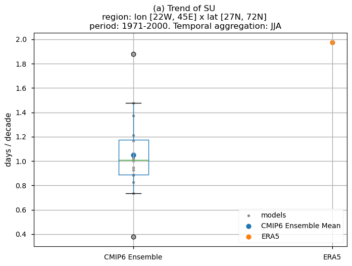
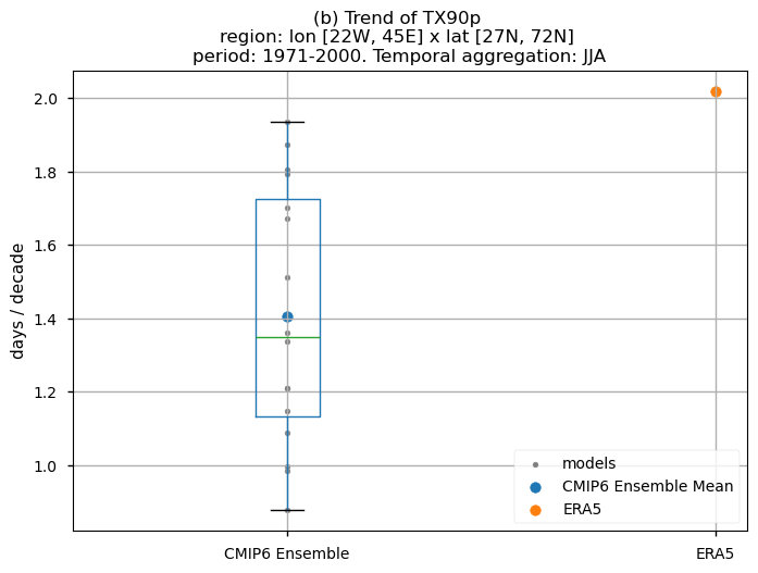
Fig 10. Boxplots illustrating the historical trends of the distribution of the chosen subset of models and ERA5 for: (a) the 'SU' index and (b) the 'TX90p' index. The distribution is created by considering spatially averaged trends across Europe. The ensemble mean and the ensemble median trends are both included. Outliers in the distribution are denoted by a grey circle with a black contour.

3.6. Results summary and discussion#

The selected subset of CMIP6 Global Climate Models (GCMs) exhibit biases in capturing both mean values and trends for the ‘number of summer days’ (SU) and ‘the number of days with daily maximum temperature exceeding the daily 90th percentile’ (TX90p) indices. These indices are calculated over the temporal aggregation of JJA and for the historical period spanning from 1971 to 2000.
GCMs struggle to accurately represent the climatology of the ‘SU’ index in regions with complex orography. Furthermore, underestimating the magnitude of this index is common, particularly in continental areas.
While the mean climate bias is mainly affected by orography, the regional variation in the trend bias is broader. ERA5 shows that the magnitude of the historical trend varies spatially. The trend bias assessment suggests that, overall, the trend is underestimated, with slight overestimations observed in certain regions. Hence, users need to consider this regional variation in both the trend and its bias.
Boxplots reveal a consistent positive spatial-averaged historical trend characterising the distribution of the chosen subset of models. Magnitudes, however, are slightly underestimated when compared to ERA5. For the ‘SU’ index, the CMIP6 ensemble median displays approximately 1.0 days/10 years, contrasting with ERA5’s ~2 days/10 years. The ‘TX90p’ index reveals around 1.4 days/10 years for the CMIP6 ensemble median in contrast to the ~2 days/10 years observed in ERA5. The interquantile range of the ensemble ranges from 0.9 to 1.2 days per decade for the ‘SU’ index (with outliers closer to 1.9 days per decade) and from 1.1 to more than 1.7 days per decade for the ‘TX90p’ index.
What do the results mean for users? Are the biases relevant?
- These results indicate that CMIP6 projections of maximum temperature indices can be useful in applications like designing strategies to optimise reinsurance protections. The findings increase confidence (though they do not ensure accuracy) when analysing future trends using these models.
- However, users must recognise that all climate projections inherently include certain biases. This is particularly important when using projections of maximum temperature indices in areas with complex orography or large continental regions. In such cases, the biases may be more pronounced and could impact the accuracy of the projections. Therefore, users should exercise caution and consider these limitations when applying the projections to their specific use cases, recognising that biases in the mean climate and trends affect indices differently and that the choice of bias correction method should be tailored accordingly [6][7].

RESULTS NOTE:
It is important to note that the results presented are specific to the 16 models chosen, and users should aim to assess as wide a range of models as possible before making a sub-selection.

If you want to know more#

Key resources#

Some key resources and further reading were linked throughout this assessment.

The CDS catalogue entries for the data used were:

CMIP6 climate projections (Daily - Daily maximum near-surface air temperature): https://cds.climate.copernicus.eu/cdsapp#!/dataset/projections-cmip6?tab=overview
ERA5 hourly data on single levels from 1940 to present (2m temperature): https://cds.climate.copernicus.eu/cdsapp#!/dataset/reanalysis-era5-single-levels?tab=overview

Code libraries used:

C3S EQC custom functions, c3s_eqc_automatic_quality_control, prepared by BOpen
icclim Python package

References#

[1] Tesselaar, M., Botzen, W.J.W., Aerts, J.C.J.H. (2020). Impacts of Climate Change and Remote Natural Catastrophes on EU Flood Insurance Markets: An Analysis of Soft and Hard Reinsurance Markets for Flood Coverage. Atmosphere 2020, 11, 146. https://doi.org/10.3390/atmos11020146.

[2] Rädler, A. T. (2022). Invited perspectives: how does climate change affect the risk of natural hazards? Challenges and step changes from the reinsurance perspective. Nat. Hazards Earth Syst. Sci., 22, 659–664. https://doi.org/10.5194/nhess-22-659-2022.

[3] Vellinga, P., Mills, E., Bowers, L., Berz, G.A., Huq, S., Kozak, L.M., Paultikof, J., Schanzenbacker, B., Shida, S., Soler, G., Benson, C., Bidan, P., Bruce, J.W., Huyck, P.M., Lemcke, G., Peara, A., Radevsky, R., Schoubroeck, C.V., Dlugolecki, A.F. (2001). Insurance and other financial services. In J. J. McCarthy, O. F. Canziani, N. A. Leary, D. J. Dokken, & K. S. White (Eds.), Climate change 2001: impacts, adaptation, and vulnerability. Contribution of working group 2 to the third assessment report of the intergovernmental panel on climate change. (pp. 417-450). Cambridge University Press.

[4] Lemos, M.C. and Rood, R.B. (2010). Climate projections and their impact on policy and practice. WIREs Clim Chg, 1: 670-682. https://doi.org/10.1002/wcc.71

[5] Nissan, H., Goddard, L., de Perez, E.C., et al. (2019). On the use and misuse of climate change projections in international development. WIREs Clim Change, 10:e579. https://doi.org/10.1002/wcc.579

[6] Iturbide, M., Casanueva, A., Bedia, J., Herrera, S., Milovac, J., Gutiérrez, J.M. (2021). On the need of bias adjustment for more plausible climate change projections of extreme heat. Atmos. Sci. Lett., 23, e1072. https://doi.org/10.1002/asl.1072

[7] https://ibicus.readthedocs.io/en/latest/.

CMIP6 Climate Projections: evaluating bias in extreme temperature indices for the reinsurance sector.

Contents

CMIP6 Climate Projections: evaluating bias in extreme temperature indices for the reinsurance sector.#

Use case: Defining a strategy to optimise reinsurance protections#

Quality assessment question#

Quality assessment statement#

Methodology#

Analysis and results#

1. Parameters, requests and functions definition#

1.1. Import packages#

1.2. Define Parameters#

1.3. Define models#

1.4. Define ERA5 request#

1.5. Define model requests#

1.6. Functions to cache#

2. Downloading and processing#

2.1. Download and transform ERA5#

2.2. Download and transform models#

2.3. Apply land-sea mask, change attributes and cut the region to show#

3. Plot and describe results#

3.1. Define plotting functions#

3.2. Plot ensemble maps#

3.3. Plot model maps#

3.4. Plot bias maps#

3.5. Boxplots of the historical trend#

3.6. Results summary and discussion#

If you want to know more#

Key resources#

References#