CMIP6 Climate Projections: evaluating uncertainty in projected changes in extreme temperature indices at a 2°C Global Warming Level for the reinsurance sector.

CMIP6 Climate Projections: evaluating uncertainty in projected changes in extreme temperature indices at a 2°C Global Warming Level for the reinsurance sector.#

Use case: Defining a strategy to optimise reinsurance protections#

Quality assessment question#

What are the projected changes for a global warming level of 2°C and associated uncertainties in air temperature extremes in Europe?

Production date: 10-07-2024

Produced by: CMCC foundation - Euro-Mediterranean Center on Climate Change. Albert Martinez Boti.

Climate change has a major impact on the reinsurance market [1][2]. In the third assessment report of the IPCC, hot temperature extremes were already presented as relevant to insurance and related services [3]. Consequently, the need for reliable regional and global climate projections has become paramount, offering valuable insights for optimising reinsurance strategies in the face of a changing climate landscape. Nonetheless, despite their pivotal role, uncertainties inherent in these projections can potentially lead to misuse [4][5]. This underscores the importance of accurately calculating and accounting for uncertainties to ensure their appropriate consideration. This notebook utilises data from CMIP6 Global Climate Models (GCM) and explores the projected changes and uncertainties in future projections of maximum temperature-based extreme indices by considering the ensemble inter-model spread of a subset of CMIP6 models at a global mean warming level of 2°C. Two maximum temperature-based indices from ECA&D indices (one of physical nature and the other of statistical nature) are computed using the icclim Python package. The first index, identified by the ETCCDI short name ‘SU’, quantifies the occurrence of summer days (i.e., with daily maximum temperatures exceeding 25°C) within a year or a season (JJA in this notebook). The second index, labeled ‘TX90p’, describes the number of days with daily maximum temperatures exceeding the daily 90th percentile of maximum temperature for a 5-day moving window. In this notebook, these calculations are performed over the historical period from 1971 to 2000 and compared to the global warming level of 2°C. The global warming level of 2°C can be defined as the first time the 30-year moving average (centre year) of global temperature is above 2°C compared to pre-industrial (Grigory Nikulin et al. (2018) [6]). The preindustrial period is defined here as the period spanning from 1861 to 1890 and the index calculations are performed for the Shared Socioeconomic Pathways SSP5-8.5. It is important to mention that the results presented here pertain to a specific subset of the CMIP6 ensemble and may not be generalisable to the entire dataset. Also note that a separate assessment examines the representation of climatology and trends of these indices for the same models during the historical period (1971-2000), while another assessment looks at the projected trends of these indices for the same models during a fixed future period (2015-2099).

Quality assessment statement#

For the CMIP6 models analysed, there is clear agreement on the sign of the climate signal for the selected indices during the JJA season, underscoring the need for proactive measures to optimise reinsurance protections in the face of projected increases in air temperature extremes for a world 2°C warmer. The advantage of using Global Warming levels (GWL of 2°C for this notebook), as opposed to considering the trend for a fixed future period, is that it eliminates the systematic biases of the models by focusing on differences rather than absolute values. However, it is important to note that the timing of the thirty-year period when the global mean temperature reaches 2°C above the preindustrial baseline varies depending on the model, making it challenging to determine.
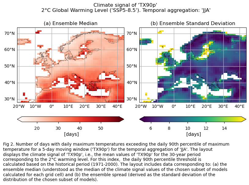
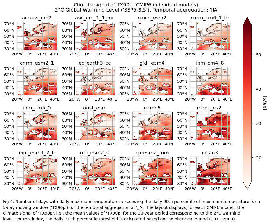
The considered subset of CMIP6 models shows that, in a world 2°C warmer than the preindustrial baseline, the average number of days with maximum daily temperatures surpassing the daily 90th percentile (calculated for the historical period) during the JJA season exhibits spatial differences across Europe. Notably, values are higher for the Mediterranean Basin, consistent with the findings of Josep Cos et al. (2022) [7], who assessed the Mediterranean climate change hotspot using CMIP6 projections. The boxplot analysis for this index displays an ensemble median spatially-averaged value over Europe larger than 32 days for the JJA season, indicating that under a 2°C global warming level, one out of every three days is projected to have a maximum daily temperature above the daily 90th percentile calculated for the historical period.
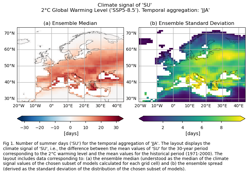
The frequency of summer days occurring during the JJA season, is projected to generally increase in a world 2°C warmer than the preindustrial baseline (1861-1890), compared to the average occurrences during the control period (1971-2000) across Europe, albeit with regional variations. Minor changes are expected in the northernmost and southern regions. In the north, where temperatures historically remain below the 25°C threshold even during the JJA season, the increase in the number of summer days is minimal (the threshold temperature of 25°C may be too high to be reached even in a world 2°C warmer than the preindustrial). In the southern Mediterranean Basin, the threshold is usually surpassed throughout the entire JJA season in the historical period, and thus, little change is observed (specially in northern Africa). This arise limitations of this index, indicating the potential need to select a higher threshold to capture the changes in these regions. Such regions, where the changes may be just as impactful or even more so than areas with a significant increase in days above 25 degrees, require careful consideration.
These findings emphasise the importance of integrating both statistical and physical extreme indices for a comprehensive assessment of climate impacts, particularly when developing adaptive strategies such as reinsurance protections. While percentile-based indices may better capture changes across all regions, they may pose challenges for users who are more used to fixed thresholds.

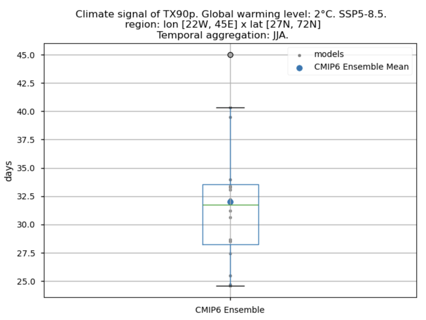
Fig A. Boxplot illustrating the climate signal (i.e., the mean values for the warming level of 2°C compared to the historical period from 1971 to 2000) for the ensemble distribution of the 'TX90p' index. For this index, the daily 90th percentile threshold is calculated based on the historical period (1971-2000). The distribution is created by considering spatially averaged values across Europe. The ensemble mean and the ensemble median are both included. Outliers in the distribution are denoted by a grey circle with a black contour.

Methodology#

This notebook provides an assessment of the projected changes and their associated uncertainties, utilising a subset of 16 models from CMIP6 under a global warming level of 2°C. The uncertainty is explored by analysing the ensemble inter-model spread of projected changes for the maximum-temperature-based indices ‘SU’ and ‘TX90p,’ calculated over the temporal aggregation of JJA for the specific global warming level of 2°C. In particular, spatial patterns of the climate signal (i.e., mean values of the indices for the warming level of 2°C compared to the historical period from 1971 to 2000) are examined and displayed for each model individually and for the ensemble median (calculated for each grid cell), alongside the ensemble inter-model spread to account for projected uncertainty. Additionally, spatially-averaged values are analysed and presented using box plots to provide an overview of climate signal behavior across the distribution of the chosen subset of models when averaged across Europe.

The analysis and results follow the next outline:

1. Parameters, requests and functions definition

1.1. Import packages
1.2. Define Parameters
1.3. Define models
1.4. Define land-sea mask request
1.5. Define model requests
1.6. Functions to cache

2. Downloading and processing

2.1. Download and transform the regridding model
2.2. Download and transform models
2.3. Apply land-sea mask, change attributes and cut the region to show

3. Plot and describe results

3.1. Define plotting functions
3.2. Plot ensemble maps
3.3. Plot model maps
3.4. Boxplots of the climate change signal
3.5. Results summary and discussion

Analysis and results#

1. Parameters, requests and functions definition#

1.1. Import packages#

1.2. Define Parameters#

In the “Define Parameters” section, various customisable options for the notebook are specified. Most of the parameters chosen are the same as those used in other assessments (“CMIP6 Climate Projections: evaluating bias in extreme temperature indices for the reinsurance sector”), being them:

historical_slice determines the historical (or control) period used (1971 to 2000 to be consistent with other user question of the same use case)
The timeseries set the temporal aggregation. For instance, selecting “JJA” implies considering only the JJA season.
The index_names parameter enables the selection of maximum-temperature-based indices (‘SU’ and ‘TX90p’ in our case) from the icclim Python package.
collection_id sets the family of models. Only CMIP6 is implemented for this notebook.
area allows specifying the geographical domain of interest.
The interpolation_method parameter allows selecting the interpolation method when regridding is performed over the indices.
The chunk selection allows the user to define if dividing into chunks when downloading the data on their local machine. Although it does not significantly affect the analysis, it is recommended to keep the default value for optimal performance.

1.3. Define models#

The following climate analyses are performed considering a subset of GCMs from CMIP6. Models names are listed in the parameters below. The selected CMIP6 models have available both the historical and SSP8.5 experiments, and are the same as those used in another assessment (“CMIP6 Climate Projections: evaluating bias in extreme temperature indices for the reinsurance sector”). Additionally, for each model, the thirty-year period corresponding to the Global Warming Level of 2°C above the preindustrial period is specified.

The Global Warming Level of 2°C can be defined as the earliest point at which a 30-year moving average of global temperature exceeds by two degrees compared to the 1861–1890 baseline [6]. This thirty-year period varies depending on the Global Climate Model being analysed. To determine this timeframe, the global mean surface temperature for the preindustrial baseline is first calculated for each model. Then, a rolling mean over 30 years is applied to the future period from 2015 to 2099, following the SSP5-8.5 scenario. Finally, the earliest 30-year period at which each model reaches the global warming level of 2°C above the preindustrial period is identified.

NOTE on the 30-year slice used for Global Warming Level calculations:
Given the 30-year duration of the historical/control period, the period of mean global surface temperature reaching 2 degrees above preindustrial levels was defined as a 30-year interval (while some studies use 20-year slices for this purpose). The pre-industrial period was also calculated as a 30-year slice (as done in [6]), despite the standard practice of considering the period from 1850 to 1900. This approach not only saves computational time but also ensures consistency in working with 30-year slices.

NOTE on the Global Warming Level calculation:
To streamline the current notebook and avoid excessive length and complexity, the calculation of the Global Warming Level of 2°C above the preindustrial period for each model has been conducted externally.

Show code cell source Hide code cell source

if collection_id == "CORDEX":
    models_cordex = {}
    raise NotImplementedError

match variable:
    case "temperature":
        index_names = ("SU", "TX90p")
        era5_variable = "2m_temperature"
        cmip6_variable = "daily_maximum_near_surface_air_temperature"
        cordex_variable = "maximum_2m_temperature_in_the_last_24_hours"
        models_cmip6 = {
            "access_cm2": slice(2022, 2051),
            "awi_cm_1_1_mr": slice(2021, 2050),
            "cmcc_esm2": slice(2024, 2053),
            "cnrm_cm6_1_hr": slice(2015, 2044),
            "cnrm_esm2_1": slice(2031, 2060),
            "ec_earth3_cc": slice(2019, 2048),
            "gfdl_esm4": slice(2037, 2066),
            "inm_cm4_8": slice(2030,2059),
            "inm_cm5_0": slice(2031, 2060),
            "kiost_esm": slice(2022,2051),
            "miroc6": slice(2039, 2068),
            "miroc_es2l": slice(2033,2062),
            "mpi_esm1_2_lr": slice(2034, 2063),
            "mri_esm2_0": slice(2023,2052),
            "noresm2_mm": slice(2040,2069),
            "nesm3": slice(2018,2047),
        }
        #Define dictionaries to use in titles and caption
        long_name = {
            "SU":"Number of summer days",
            "TX90p":"Number of days with daily maximum temperatures exceeding the daily 90th percentile of maximum temperature for a 5-day moving window",
        }
        # Colormaps
        cmaps = {"SU": "RdBu_r", "TX90p": "Reds"}
    case "precipitation":
        index_names = ("CWD", "R20mm", "RR1", "RX1day", "RX5day")
        era5_variable = "total_precipitation"
        cmip6_variable = "precipitation"
        cordex_variable = "mean_precipitation_flux"
        models_cmip6 = {
            "access_cm2": slice(2022, 2051),
            "bcc_csm2_mr": slice(2025, 2054),
            "cmcc_esm2": slice(2024, 2053),
            "cnrm_cm6_1_hr": slice(2015, 2044),
            "cnrm_esm2_1": slice(2031, 2060),
            "ec_earth3_cc": slice(2019, 2048),
            "gfdl_esm4": slice(2037, 2066),
            "inm_cm4_8": slice(2030,2059),
            "inm_cm5_0": slice(2031, 2060),
            "miroc6": slice(2039, 2068),
            "miroc_es2l": slice(2033,2062),
            "mpi_esm1_2_lr": slice(2034, 2063),
            "mri_esm2_0": slice(2023,2052),
            "noresm2_mm": slice(2040,2069),
            "nesm3": slice(2018,2047),
            "ukesm1_0_ll": slice(2017,2046),
        }
        #Define dictionaries to use in titles and caption
        long_name = {
            "RX1day": "Maximum 1-day total precipitation",
            "RX5day": "Maximum 5-day total precipitation",
            "RR1":"Number of wet days (Precip >= 1mm)",
            "R20mm":"Number of heavy precipitation days (Precip >= 20mm)",
            "CWD":"Maximum consecutive wet days",
        }
        # Colormaps
        cmaps = "RdBu"
    case _:
        raise NotImplementedError(f"{variable=}")

model_regrid = "gfdl_esm4" 

1.4. Define land-sea mask request#

Within this notebook, ERA5 will be used to download the land-sea mask when plotting. In this section, we set the required parameters for the cds-api data-request of ERA5 land-sea mask.

1.5. Define model requests#

In this section we set the required parameters for the cds-api data-request.

When Weights = True, spatial weighting is applied for calculations requiring spatial data aggregation. This is particularly relevant for CMIP6 GCMs with regular lon-lat grids that do not consider varying surface extensions at different latitudes. In contrast, CORDEX RCMs, using rotated grids, inherently account for different cell surfaces based on latitude, eliminating the need for a latitude cosine multiplicative factor (Weights = False).

1.6. Functions to cache#

In this section, functions that will be executed in the caching phase are defined. Caching is the process of storing copies of files in a temporary storage location, so that they can be accessed more quickly. This process also checks if the user has already downloaded a file, avoiding redundant downloads.

Functions description:

The select_timeseries function subsets the dataset based on the chosen timeseries parameter, which could be a specific season (e.g., “JJA”) or “annual.” It tailors the dataset according to the specified criteria, providing either annual or seasonal data as the outcome.
The compute_indices function utilises the icclim package to calculate the selected maximum-temperature-based indices.
Finally, the compute_indices_and_trends function selects the temporal aggregation using the select_timeseries function. It then calculates maximum-temperature-based indices via the compute_indices function and determines the indices mean over the period of interest.

Show code cell source Hide code cell source

def select_timeseries(ds, timeseries, year_slice, index_names):
    if timeseries == "annual":
        return ds.sel(time=slice(str(year_slice.start), str(year_slice.stop)))
    ds=ds.sel(time=slice(f"{year_slice.start-1}-12", f"{year_slice.stop}-11"))
    if "RX5day" in index_names:
        return ds
    return ds.where(ds["time"].dt.season == timeseries, drop=True)


def compute_indices(
    ds,
    index_names,
    timeseries,
    tmpdir,
    historical_slice,
    future_slice,
):
    labels, datasets = zip(*ds.groupby("time.year"))
    paths = [f"{tmpdir}/{label}.nc" for label in labels]
    datasets = [ds.chunk(-1) for ds in datasets]
    xr.save_mfdataset(datasets, paths)

    ds = xr.open_mfdataset(paths)
    in_files = f"{tmpdir}/rechunked.zarr"
    chunks = {dim: -1 if dim == "time" else "auto" for dim in ds.dims}
    ds.chunk(chunks).to_zarr(in_files)

    future_range = (f"{future_slice.start}-01-01", f"{future_slice.stop}-12-31")
    historical_range = (
        f"{historical_slice.start}-01-01",
        f"{historical_slice.stop}-12-31",
    )

    datasets = []
    for index_name in index_names:
        kwargs = {
            "index_name": index_name,
            "in_files": in_files,
            "slice_mode": "year" if timeseries == "annual" else timeseries,
        }
        if index_name == "TX90p":
            datasets.append(
                icclim.index(
                    out_file=f"{tmpdir}/{index_name}.nc",
                    time_range=future_range,
                    base_period_time_range=historical_range,
                    **kwargs,
                )
            )
        else:
            ds_historical = icclim.index(
                out_file=f"{tmpdir}/{index_name}_historical.nc",
                time_range=historical_range,
                **kwargs,
            )
            ds_future = icclim.index(
                out_file=f"{tmpdir}/{index_name}_future.nc",
                time_range=future_range,
                **kwargs,
            )
            with xr.set_options(keep_attrs=True):
                datasets.append(ds_future.mean("time") - ds_historical.mean("time"))
    return xr.merge(datasets).drop_dims("bounds")


def add_bounds(ds):
    for coord in {"latitude", "longitude"} - set(ds.cf.bounds):
        ds = ds.cf.add_bounds(coord)
    return ds


def get_grid_out(request_grid_out, method):
    ds_regrid = download.download_and_transform(*request_grid_out)
    coords = ["latitude", "longitude"]
    if method == "conservative":
        ds_regrid = add_bounds(ds_regrid)
        for coord in list(coords):
            coords.extend(ds_regrid.cf.bounds[coord])
    grid_out = ds_regrid[coords]
    coords_to_drop = set(grid_out.coords) - set(coords) - set(grid_out.dims)
    grid_out = ds_regrid[coords].reset_coords(coords_to_drop, drop=True)
    grid_out.attrs = {}
    return grid_out


def compute_indices_and_trends_future_vs_historical(
    ds,
    index_names,
    timeseries,
    historical_slice,
    future_slice,
    request_grid_out=None,
    **regrid_kwargs,
):
    assert (request_grid_out and regrid_kwargs) or not (
        request_grid_out or regrid_kwargs
    )
    ds = ds.drop_vars([var for var, da in ds.data_vars.items() if len(da.dims) != 3])
    ds = ds[list(ds.data_vars)]

    # Original bounds for conservative interpolation
    if regrid_kwargs.get("method") == "conservative":
        ds = add_bounds(ds)
        bounds = [
            ds.cf.get_bounds(coord).reset_coords(drop=True)
            for coord in ("latitude", "longitude")
        ]
    else:
        bounds = []

    ds_historical = select_timeseries(ds, timeseries, historical_slice,index_names)
    ds_future = select_timeseries(ds, timeseries, future_slice,index_names)
    ds = xr.concat([ds_historical, ds_future], "time")
    with tempfile.TemporaryDirectory() as tmpdir:
        ds = compute_indices(
            ds, index_names, timeseries, tmpdir, historical_slice, future_slice
        )
        ds = ds.mean("time", keep_attrs=True).compute()
        if request_grid_out:
            ds = diagnostics.regrid(
                ds.merge({da.name: da for da in bounds}),
                grid_out=get_grid_out(request_grid_out, regrid_kwargs["method"]),
                **regrid_kwargs,
            )
        return ds

2. Downloading and processing#

2.1. Download and transform the regridding model#

In this section, the download.download_and_transform function from the ‘c3s_eqc_automatic_quality_control’ package is employed to download daily data from the selected CMIP6 regridding model, compute the indices for the selected temporal aggregation (“JJA” in our example), calculate the mean for the historical period (1971-2000) and for the thirty-year period corresponding to the 2°C Global Warming Level, and cache the result (to avoid redundant downloads and processing).

The regridding model is intended here as the model whose grid will be used to interpolate the others. This ensures all models share a common grid, facilitating the calculation of median values for each cell point. The regridding model within this notebook is “gfdl_esm4” but a different one can be selected by just modifying the model_regrid parameter at 1.3. Define models. It is key to highlight the importance of the chosen target grid depending on the specific application.

NOTE on the Global Warming Level calculation:
The thirty year-period corresponding to the 2°C Global Warming Level is different for each model. Its calculation has been conducted externally.

2.2. Download and transform models#

In this section, we utilise the download_and_transform function from the ‘c3s_eqc_automatic_quality_control’ package to download daily data from the CMIP6 models for the historical period (1971-2000) and for the thirty-year period corresponding to the 2°C warming level of each model. Subsequently, temporal aggregation is selected (in our example, ‘JJA’). The next step involves calculating the indices and the climate signal. For the ‘SU’ index, as we are dealing with an index calculated using a physical threshold, the climate signal is obtained as the difference between the mean values for the thirty-year period corresponding to the 2°C Global Warming Level and the mean values calculated over the historical period (1971-2000). The climate signal for the ‘TX90p’ index, as we are dealing with an index based on a statistical threshold, is obtained by calculating - for the thirty-year period corresponding to the 2°C warming level - the mean number of days with daily maximum temperatures exceeding the daily 90th percentile. The daily 90th percentile threshold is calculated based on the historical period of 1971-2000.

NOTE on the Global Warming Level calculation:
The thirty year-period corresponding to the 2°C Global Warming Level is different for each model. Its calculation has been conducted externally.

model='access_cm2'
model='awi_cm_1_1_mr'
model='cmcc_esm2'
model='cnrm_cm6_1_hr'
model='cnrm_esm2_1'
model='ec_earth3_cc'
model='gfdl_esm4'
model='inm_cm4_8'
model='inm_cm5_0'
model='kiost_esm'
model='miroc6'
model='miroc_es2l'
model='mpi_esm1_2_lr'
model='mri_esm2_0'
model='noresm2_mm'
model='nesm3'

2.3. Apply land-sea mask, change attributes and cut the region to show#

This section performs the following tasks:

Cut the region of interest.
Downloads the sea mask for ERA5.
Regrids ERA5’s mask to the model_regrid grid and applies it to the regridded data
Regrids the ERA5 land-sea mask to the model’s original grid and applies it to them.
Change some variable attributes for plotting purposes.

Note: ds_interpolated contains data from the models regridded to the regridding model’s grid. model_datasets contain the same data but in the original grid of each model.

3. Plot and describe results#

This section will display the following results:

Maps representing the spatial distribution of the climate change signal (i.e., mean values for the warming level of 2°C compared to the historical period 1971-2000) of the indices ‘SU’ and ‘TX90p’ for each model individually, the ensemble median (understood as the median of the climate signal values of the chosen subset of models calculated for each grid cell), and the ensemble spread (derived as the standard deviation of the distribution of the chosen subset of models).
Boxplots representing statistical distributions (PDFs) constructed from the spatially-averaged climate signal of each considered model.

3.1. Define plotting functions#

The functions presented here are used to plot the climate signal (i.e., the mean values for the warming level of 2°C compared to the historical period) for each of the indices (‘SU’ and ‘TX90p’).

For a selected index, two layout types will be displayed, depending on the chosen function:

Layout including the ensemble median and the ensemble spread: plot_ensemble() is used.
Layout including every model: plot_models() is employed.

Show code cell source Hide code cell source

#Define function to plot the caption of the figures (for the ensmble case)
def add_caption_ensemble(index):
    #Add caption to the figure
    match index:
        case "TX90p":
            caption_text = (
                f"Fig {fig_number}. {long_name[index]} ('{index}') for "
                f"the temporal aggregation of '{timeseries}'. The layout displays "
                f"the climate signal of '{index}', i.e., the mean values of '{index}' "
                f"for the 30-year period corresponding to the 2°C warming level. For this index,  "
                f"the daily 90th percentile threshold is calculated based on the historical period (1971-2000). "
                f"The layout includes data corresponding to: (a) the ensemble median (understood as the median "
                f"of the climate signal values of the chosen subset of models " 
                f"calculated for each grid cell) and (b) the ensemble spread "
                f"(derived as the standard deviation of the distribution of the chosen " 
                f"subset of models)."
            )
        case _:
            caption_text = (
                f"Fig {fig_number}. {long_name[index]} ('{index}') for "
                f"the temporal aggregation of '{timeseries}'. The layout displays "
                f"the climate signal of '{index}', i.e., the difference between the mean values of '{index}' "
                f"for the 30-year period corresponding to the 2°C warming level and the mean values for the "
                f"historical period (1971-2000). " 
                f"The layout includes data corresponding to: (a) the ensemble median (understood as the median "
                f"of the climate signal values of the chosen subset of models " 
                f"calculated for each grid cell) and (b) the ensemble spread "
                f"(derived as the standard deviation of the distribution of the chosen " 
                f"subset of models)."
            ) 
            
    wrapped_lines = textwrap.wrap(caption_text, width=105)
    # Add each line to the figure
    for i, line in enumerate(wrapped_lines):
        fig.text(0, -0.05  - i * 0.03, line, ha='left', fontsize=10)
    #end captioning


#Define function to plot the cation of the figures (for the individual models case)
def add_caption_models(index):
    #Add caption to the figure
    match index:
        case "TX90p":
            caption_text = (
                f"Fig {fig_number}. {long_name[index]} ('{index}') for the temporal aggregation of "
                f"'{timeseries}'. The layout displays, for each {collection_id} model,  "
                f"the climate signal of '{index}', i.e., the mean values of '{index}' "
                f"for the 30-year period corresponding to the 2°C warming level. For this index, the daily "
                f" 90th percentile threshold is calculated based on the historical period (1971-2000). "
            )
        case _:
            caption_text = (
                f"Fig {fig_number}. {long_name[index]} ('{index}') for the temporal aggregation of "
                f"'{timeseries}'. The layout displays, for each {collection_id} model,  "
                f"the climate signal of '{index}', i.e., the difference between the mean values of '{index}' "
                f"for the 30-year period corresponding to the 2°C warming level and the mean values "
                f"for the historical period (1971-2000)"
            )
    wrapped_lines = textwrap.wrap(caption_text, width=120)
    # Add each line to the figure
    for i, line in enumerate(wrapped_lines):
        fig.text(0, -0.05  - i * 0.03, line, ha='left', fontsize=10)

def hatch_p_value(da, ax, **kwargs):
    default_kwargs = {
        "plot_func": "contourf",
        "show_stats": False,
        "cmap": "none",
        "add_colorbar": False,
        "levels": [0, 0.05, 1],
        "hatches": ["", "/" * 3],
    }
    kwargs = default_kwargs | kwargs

    title = ax.get_title()
    plot_obj = plot.projected_map(da, ax=ax, **kwargs)
    ax.set_title(title)
    return plot_obj


def hatch_p_value_ensemble(trend, p_value, ax):
    n_models = trend.sizes["model"]
    robust_ratio = (p_value <= 0.05).sum("model") / n_models
    robust_ratio = robust_ratio.where(p_value.notnull().any("model"))
    signs = xr.concat([(trend > 0).sum("model"), (trend < 0).sum("model")], "sign")
    sign_ratio = signs.max("sign") / n_models
    robust_threshold = 0.66
    sign_ratio = sign_ratio.where(robust_ratio > robust_threshold)
    for da, threshold, character in zip(
        [robust_ratio, sign_ratio], [robust_threshold, 0.8], ["/", "\\"]
    ):
        hatch_p_value(da, ax=ax, levels=[0, threshold, 1], hatches=[character * 3, ""])


def set_extent(da, axs, area):
    extent = [area[i] for i in (1, 3, 2, 0)]
    for i, coord in enumerate(extent):
        extent[i] += -1 if i % 2 else +1
    for ax in axs:
        ax.set_extent(extent)


def plot_models(
    data,
    da_for_kwargs=None,
    p_values=None,
    col_wrap=4 if collection_id=="CMIP6" else 3,
    subplot_kw={"projection": ccrs.PlateCarree()},
    figsize=None,
    layout="constrained",
    area=area,
    **kwargs,
):
    if isinstance(data, dict):
        assert da_for_kwargs is not None
        model_dataarrays = data
    else:
        da_for_kwargs = da_for_kwargs or data
        model_dataarrays = dict(data.groupby("model"))

    if p_values is not None:
        model_p_dataarrays = (
            p_values if isinstance(p_values, dict) else dict(p_values.groupby("model"))
        )
    else:
        model_p_dataarrays = None

    # Get kwargs
    default_kwargs = {"robust": True, "extend": "both"}
    kwargs = default_kwargs | kwargs
    kwargs = xr.plot.utils._determine_cmap_params(da_for_kwargs.values, **kwargs)

    fig, axs = plt.subplots(
        *(col_wrap, math.ceil(len(model_dataarrays) / col_wrap)),
        subplot_kw=subplot_kw,
        figsize=figsize,
        layout=layout,
    )
    axs = axs.flatten()
    for (model, da), ax in zip(model_dataarrays.items(), axs):
        pcm = plot.projected_map(
            da, ax=ax, show_stats=False, add_colorbar=False, **kwargs
        )
        ax.set_title(model)
        if model_p_dataarrays is not None:
            hatch_p_value(model_p_dataarrays[model], ax)
    set_extent(da_for_kwargs, axs, area)
    fig.colorbar(
        pcm,
        ax=axs.flatten(),
        extend=kwargs["extend"],
        location="right",
        label=f"{da_for_kwargs.attrs.get('long_name', '')} [{da_for_kwargs.attrs.get('units', '')}]",
    )
    return fig


def plot_ensemble(
    da_models,
    da_era5=None,
    p_value_era5=None,
    p_value_models=None,
    subplot_kw={"projection": ccrs.PlateCarree()},
    figsize=None,
    layout="constrained",
    cbar_kwargs=None,
    area=area,
    cmap_bias=None,
    cmap_std=None,
    **kwargs,
):
    # Get kwargs
    default_kwargs = {"robust": True, "extend": "both"}
    kwargs = default_kwargs | kwargs
    kwargs = xr.plot.utils._determine_cmap_params(
        da_models.values if da_era5 is None else da_era5.values, **kwargs
    )
    if da_era5 is None and cbar_kwargs is None:
        cbar_kwargs = {"orientation": "horizontal"}

    # Figure
    fig, axs = plt.subplots(
        *(1 if da_era5 is None else 2, 2),
        subplot_kw=subplot_kw,
        figsize=figsize,
        layout=layout,
    )
    axs = axs.flatten()
    axs_iter = iter(axs)

    # ERA5
    if da_era5 is not None:
        ax = next(axs_iter)
        plot.projected_map(
            da_era5, ax=ax, show_stats=False, cbar_kwargs=cbar_kwargs, **kwargs
        )
        if p_value_era5 is not None:
            hatch_p_value(p_value_era5, ax=ax)
        ax.set_title("(a) ERA5")

    # Median
    ax = next(axs_iter)
    median = da_models.median("model", keep_attrs=True)
    plot.projected_map(
        median, ax=ax, show_stats=False, cbar_kwargs=cbar_kwargs, **kwargs
    )
    if p_value_models is not None:
        hatch_p_value_ensemble(trend=da_models, p_value=p_value_models, ax=ax)
    ax.set_title("(b) Ensemble Median" if da_era5 is not None else "(a) Ensemble Median")

    # Bias
    if da_era5 is not None:
        ax = next(axs_iter)
        with xr.set_options(keep_attrs=True):
            bias = median - da_era5
        plot.projected_map(
            bias,
            ax=ax,
            show_stats=False,
            center=0,
            cbar_kwargs=cbar_kwargs,
            **(default_kwargs | {"cmap": cmap_bias}),
        )
        ax.set_title("(c) Ensemble Median Bias")

    # Std
    ax = next(axs_iter)
    std = da_models.std("model", keep_attrs=True)
    plot.projected_map(
        std,
        ax=ax,
        show_stats=False,
        cbar_kwargs=cbar_kwargs,
        **(default_kwargs | {"cmap": cmap_std}),
    )
    ax.set_title("(d) Ensemble Standard Deviation" if da_era5 is not None else "(b) Ensemble Standard Deviation")

    set_extent(da_models, axs, area)
    return fig

3.2. Plot ensemble maps#

In this section, we invoke the plot_ensemble() function to visualise the climate signal (i.e., the mean values for the warming level of 2°C compared to the historical period) across Europe for each of the indices (‘SU’ and ‘TX90p’). The layout includes: (a) the ensemble median (understood as the median of the climate signal values of the chosen subset of models calculated for each grid cell) and (b) the ensemble spread (derived as the standard deviation of the distribution of the chosen subset of models).

Note that the model data used in this section has previously been interpolated to the “regridding model” grid ("gfdl_esm4" for this notebook).

../_images/2cafb539eef362834e690c5d7ef09ff80a1c0bcb0579c47fb4b156cc1ecb94f2.png

../_images/4c48616c5be2d8781719b3c54b72aced3f1917e00a89b3b1a013f7480d2d1716.png

3.3. Plot model maps#

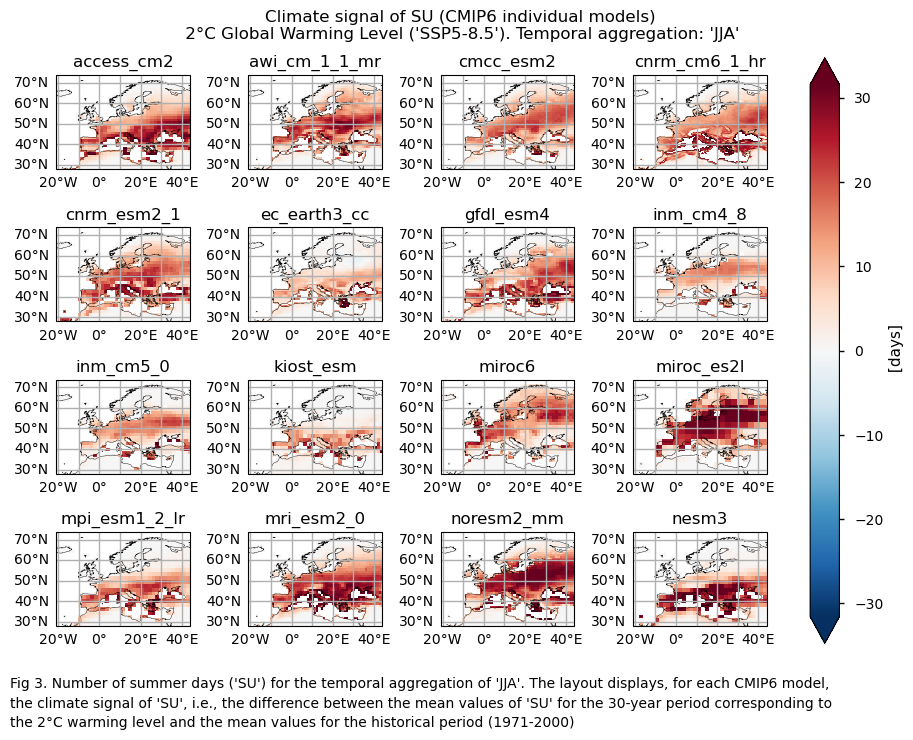
In this section, we invoke the plot_models() function to visualise the climate signal for every model individually across Europe. Note that the model data used in this section maintains its original grid.

Specifically, for each of the indices (‘SU’ and ‘TX90p’), this section presents a single layout including the climate signal of every model.

../_images/ad317df7094230a0e483a8cd49f52c1353354cd88bb9e2cac7283bb595a0fd83.png

../_images/965b4a127b71c7256517b655f1c17f945c9d7bf23e44d10e6b8fc24099e821af.png

3.4. Boxplots of the climate change signal#

Finally, we present boxplots representing the ensemble distribution of each climate model signal for the 2°C global warming level.

Dots represent the spatially-averaged climate signal over the selected region for each model (grey) and the ensemble mean (blue). The ensemble median is shown as a green line. Note that the spatially averaged values are calculated for each model from its original grid (i.e., no interpolated data has been used here).

The boxplot visually illustrates the distribution of the climate signal among the climate models, with the box covering the first quartile (Q1 = 25th percentile) to the third quartile (Q3 = 75th percentile), and a green line indicating the ensemble median (Q2 = 50th percentile). Whiskers extend from the edges of the box to show the full data range.

../_images/5a88108ba42651b6e710a76f7ffe9c52585ff5eb17fcaff9472a6dc6b3854ed8.png

../_images/aaad0c661ddd2c55f87fa00e6e667b49a092034260595944b7ed68aa32a05068.png

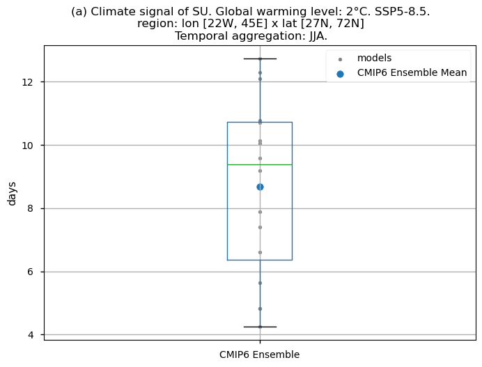
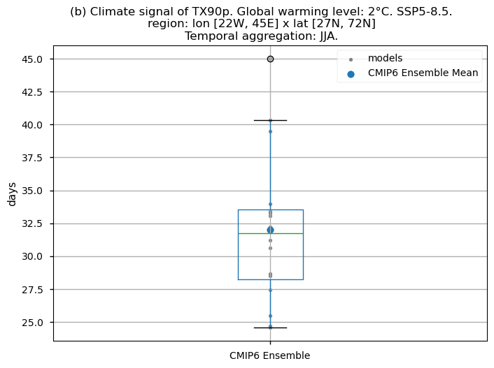
Fig 5. Boxplots illustrating the climate signal (i.e., mean values for the warming level of 2°C compared to the historical period from 1971 to 2000) of the distribution of the chosen subset of models for: (a) the 'SU' index, and (b) the 'TX90p' index. The distribution is created by considering spatially averaged values across Europe. The ensemble mean and the ensemble median are both included. Outliers in the distribution are denoted by a grey circle with a black contour.

3.5. Results summary and discussion#

The frequency of mean summer days occurring during the JJA season, defined as those with a daily maximum temperature exceeding 25°C, is projected to generally increase in a world 2°C warmer than the preindustrial baseline (1861-1890), compared to the average occurrences during the control period (1971-2000) across Europe, albeit with regional variations. Minor changes are expected in the northernmost and southern regions. In the north, where temperatures historically remain below the 25°C threshold even during the JJA season, the increase in the number of summer days is minimal (the threshold temperature of 25°C may be too high to be reached even in a world 2°C warmer than the preindustrial). In the southern Mediterranean Basin, the threshold is already surpassed throughout the entire JJA season in the historical period, and thus, no change is observed. This underscores the importance of incorporating both statistical and physical extreme indices for a comprehensive assessment of climate impacts.
The ensemble median spatially-averaged value shown through the boxplot indicates that with a 2°C global warming, the count of summer days (‘SU’) is projected to rise by approximately 10 days compared to the historical average for the JJA season. The interquartile range for the ‘SU’ index extends from around 6 to almost 11 days.
In a world 2°C warmer than the preindustrial baseline, the average number of days with maximum daily temperatures surpassing the reference 90th percentile (calculated for the historical period) during the JJA season exhibits spatial differences across Europe. Notably, values are higher for the Mediterranean Basin, consistent with the findings of Josep Cos et al. (2022) [6], who assessed the Mediterranean climate change hotspot using CMIP6 projections. The boxplot analysis for this index displays an ensemble median spatially-averaged value over Europe larger than 32 days for the JJA season, indicating that under a 2°C global warming level, one out of every three days will have a maximum daily temperature above the 90th percentile reference calculated for the historical period. The interquartile range spans approximately 28 to 33 days for the ‘TX90p’ index.
It is important to highlight that the boxplots reflect spatially-averaged values, and their outputs should be interpreted with caution, as the results may vary substantially when considering different regions across Europe.
What do the results mean for users? Are the biases from the historical notebook (“CMIP6 Climate Projections: evaluating bias in extreme temperature indices for the reinsurance sector”) relevant? What are the differences compared to looking at the trend for a fixed future period?
- For the CMIP6 models analysed, there is clear agreement on the sign of the projected climate signal, defined as the differences between the mean values of the indices calculated for a centered thirty-year period when the global mean temperature is 2°C higher than the preindustrial baseline and the mean values for the historical period from 1971 to 2000. This agreement suggests that it may be safe to include this information when designing strategies to optimise reinsurance protections in a world 2°C warmer than the preindustrial baseline.
- The advantage of using this approach, instead of considering the trend for a fixed future period, is that some of the systematic biases of the models may be removed [7], as we are dealing with differences rather than absolute values. However, it is important to note that the centered thirty-year period when the global mean temperature reaches 2°C above the preindustrial baseline varies depending on the model considered, and determining this timing can be challenging.

RESULTS NOTE:
It is important to note that the results presented are specific to the 16 models chosen, and users should aim to assess as wide a range of models as possible before making a sub-selection.

If you want to know more#

Key resources#

Some key resources and further reading were linked throughout this assessment.

The CDS catalogue entries for the data used were:

CMIP6 climate projections (Daily - Daily maximum near-surface air temperature): https://cds.climate.copernicus.eu/cdsapp#!/dataset/projections-cmip6?tab=overview

Code libraries used:

C3S EQC custom functions, c3s_eqc_automatic_quality_control, prepared by BOpen
icclim Python package

References#

[1] Tesselaar, M., Botzen, W.J.W., Aerts, J.C.J.H. (2020). Impacts of Climate Change and Remote Natural Catastrophes on EU Flood Insurance Markets: An Analysis of Soft and Hard Reinsurance Markets for Flood Coverage. Atmosphere 2020, 11, 146. https://doi.org/10.3390/atmos11020146.

[2] Rädler, A. T. (2022). Invited perspectives: how does climate change affect the risk of natural hazards? Challenges and step changes from the reinsurance perspective. Nat. Hazards Earth Syst. Sci., 22, 659–664. https://doi.org/10.5194/nhess-22-659-2022.

[3] Vellinga, P., Mills, E., Bowers, L., Berz, G.A., Huq, S., Kozak, L.M., Paultikof, J., Schanzenbacker, B., Shida, S., Soler, G., Benson, C., Bidan, P., Bruce, J.W., Huyck, P.M., Lemcke, G., Peara, A., Radevsky, R., Schoubroeck, C.V., Dlugolecki, A.F. (2001). Insurance and other financial services. In J. J. McCarthy, O. F. Canziani, N. A. Leary, D. J. Dokken, & K. S. White (Eds.), Climate change 2001: impacts, adaptation, and vulnerability. Contribution of working group 2 to the third assessment report of the intergovernmental panel on climate change. (pp. 417-450). Cambridge University Press.

[4] Lemos, M.C. and Rood, R.B. (2010). Climate projections and their impact on policy and practice. WIREs Clim Chg, 1: 670-682. https://doi.org/10.1002/wcc.71

[5] Nissan H, Goddard L, de Perez EC, et al. (2019). On the use and misuse of climate change projections in international development. WIREs Clim Change, 10:e579. https://doi.org/10.1002/wcc.579

[6] Nikulin, G., Lennard, C., Dosio, A., Kjellström, E., Chen, Y., Hänsler, A., Kupiainen, M., Laprise, R., Laura Mariotti, L., Maule C.F., et al. (2018). The effects of 1.5 and 2 degrees of global warming on Africa in the CORDEX ensemble. Environ. Res. Lett. 13 065003. https://dx.doi.org/10.1088/1748-9326/aab1b1

[7] Cos, J., Doblas-Reyes, F., Jury, M., Marcos, R., Bretonnière, P.-A., and Samsó, M. (2022). The Mediterranean climate change hotspot in the CMIP5 and CMIP6 projections, Earth Syst. Dynam., 13, 321–340. https://doi.org/10.5194/esd-13-321-2022.

CMIP6 Climate Projections: evaluating uncertainty in projected changes in extreme temperature indices at a 2°C Global Warming Level for the reinsurance sector.

Contents

CMIP6 Climate Projections: evaluating uncertainty in projected changes in extreme temperature indices at a 2°C Global Warming Level for the reinsurance sector.#

Use case: Defining a strategy to optimise reinsurance protections#

Quality assessment question#

Quality assessment statement#

Methodology#

Analysis and results#

1. Parameters, requests and functions definition#

1.1. Import packages#

1.2. Define Parameters#

1.3. Define models#

1.4. Define land-sea mask request#

1.5. Define model requests#

1.6. Functions to cache#

2. Downloading and processing#

2.1. Download and transform the regridding model#

2.2. Download and transform models#

2.3. Apply land-sea mask, change attributes and cut the region to show#

3. Plot and describe results#

3.1. Define plotting functions#

3.2. Plot ensemble maps#

3.3. Plot model maps#

3.4. Boxplots of the climate change signal#

3.5. Results summary and discussion#

If you want to know more#

Key resources#

References#