Testing the capability of CMIP6 GCMs to represent precipitation intra-seasonal variability

5.1.1. Testing the capability of CMIP6 GCMs to represent precipitation intra-seasonal variability#

Production date: 31-03-2025

Produced by: CMCC foundation - Euro-Mediterranean Center on Climate Change. Albert Martinez Boti.

Most research has focused on projected long-term changes in mean climate and extremes, while changes in variability have received less attention. However, understanding the evolution of precipitation variability is crucial for accurately modelling climate phenomena and quantifying the impacts of climate change, particularly on water resources and related socioeconomic factors [1], [2]. This notebook evaluates the capability of a subset of 16 CMIP6 Global Climate Models (GCMs) to represent monsoon intra-seasonal variability over the Indian subcontinent. Specifically, it evaluates the High-Frequency Intra-Seasonal Oscillations (HFISOs) with a characteristic period of 10–20 days, generally associated with the Quasi-Biweekly Oscillation (QBWO) [3], [4], [5]. The Low-Frequency Intra-Seasonal Oscillations (LFISOs) — which have a characteristic period of 30–60 days [6], [7] and are usually linked to the well-known Madden-Julian Oscillation (MJO) mode — are also studied.

Systematic errors are obtained by comparing LFISOs and HFISOs — calculated from model daily outputs — with those from the ERA5 reanalysis, which serves as the reference dataset. These oscillations are extracted by applying a pass-band filter (10–20 days for HFISOs and 30–60 days for LFISOs) to daily precipitation anomalies. To assess the intensity of these oscillations [8] , variance and the coefficient of variation of the filtered data are calculated for the summer monsoon period (JJAS) from 1940 to 2014. This assessment presents the spatial patterns of the variance and coefficient of variation of LFISOs and HFISOs, as well as their evolution. The latter is evaluated through time series of spatially averaged variance and coefficient of variation of the filtered data using 30-year moving windows.

Biases and future changes in LFISOs and HFISOs are highly relevant to users, as these modes are often associated with: (1) active-break cycles (i.e., alternating ‘active’ phases of heavy rainfall and quiescent phases during the peak monsoon season in July and August [9], [10]), (2) the activity of synoptic systems such as monsoon lows (e.g., [11]) and (3) late monsoon rainfall [12]. This evaluation complements another assessment that examined the representation of historic inter-annual precipitation variability across the Indian subcontinent.

🌍 Use case: Assessing the potential impacts of climate change on precipitation variability over India#

❓ Quality assessment question#

How well do CMIP6 projections represent historical intra-seasonal variability of Monsoon precipitation across the Indian subcontinent? Are there trends affecting the intra-seasonal variability of Monsoon precipitation?

📢 Quality assessment statement#

These are the key outcomes of this assessment

This assessment complements a previous analysis of historical inter-annual precipitation variability across the Indian subcontinent.
Intra-seasonal and inter-annual variability assessments show similar spatial patterns, suggesting a connection between the two [10]
Variability formulation matters: the two metrics used highlight different spatial features of intra-seasonal variability.
Variance shows model-dependent biases linked to orography and wet regions. The Coefficient of Variation (CV) normalises for mean precipitation but can lead to artificially high values in extremely dry areas.
CV differences between models are smaller than those for variance. Most models underestimate CV in dry inland regions.
HFISOs and LFISOs variance and CV exhibit similar spatial patterns.
CMIP6 models poorly capture observed trends in HFISO and LFISO variability. ERA5 shows decreasing variance and increasing CV, which are not reproduced by the ensemble median.
Bias correction may be necessary before using CMIP6 precipitation projections in water management applications. Similarities in inter-annual and intra-seasonal variability biases suggest corrections may be required at the daily level.

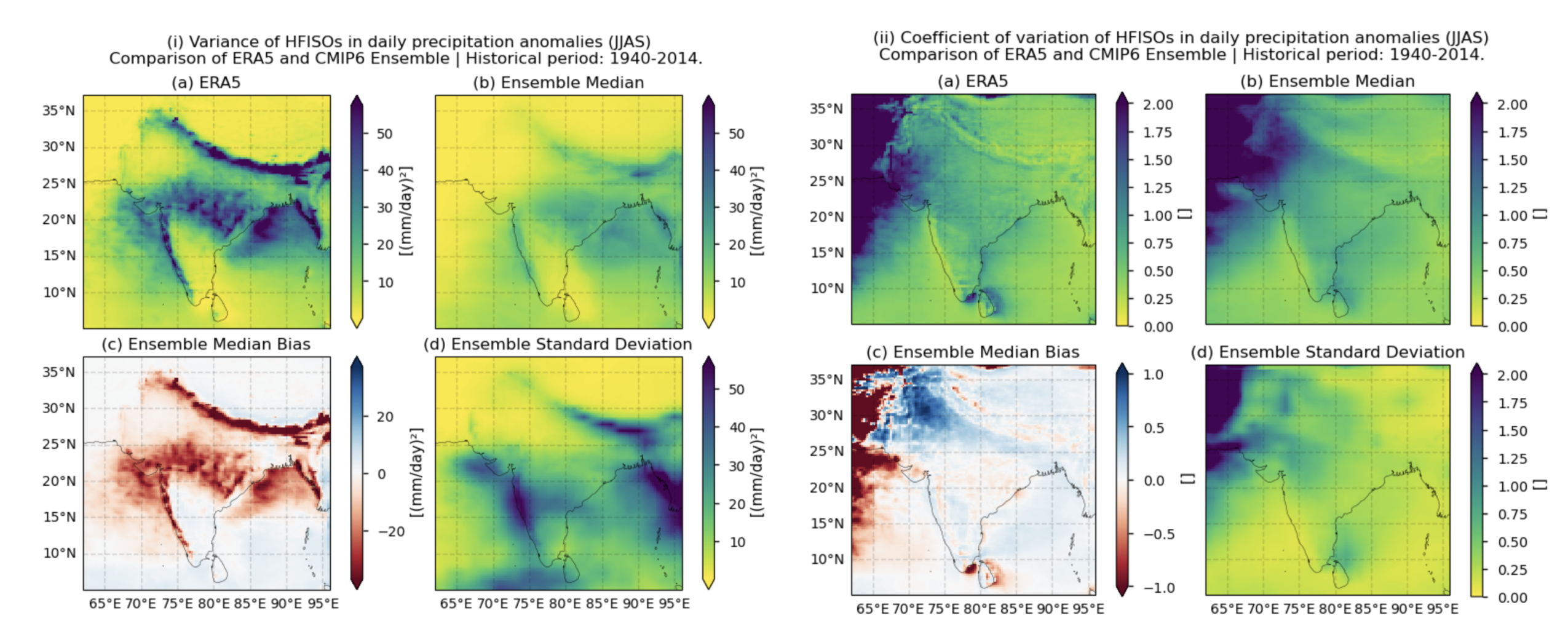
Mean Bias variance — Fig. 5.1.1.1 Fig A. i. Variance of HFISOs in daily precipitation anomalies over the historical period (1940–2014). The layout includes data corresponding to: (a) ERA5, (b) the ensemble median (defined as the median of the Variance of HFISOs values for the selected subset of models, calculated for each grid cell), (c) the bias of the ensemble median, and (d) the ensemble spread (calculated as the standard deviation of the Variance of HFISOs values for the selected subset of models). Before calculating the variance, a Lanczos band-pass filter has been applied to the daily precipitation anomalies to isolate the 10–20-day high-frequency intraseasonal oscillations (HFISOs). Fig A.ii. Same as Fig. A.i. but for the coefficient of variation of HFISOs.#

📋 Methodology#

A subset of 16 models from the CMIP6 project is used to evaluate the representation of intra-seasonal precipitation variability over the Indian subcontinent. The analysis focuses on two intra-seasonal timescales: High-Frequency Intra-Seasonal Oscillations (HFISOs) with periods of 10–20 days and Low-Frequency Intra-Seasonal Oscillations (LFISOs) with periods of 30–60 days. LFISOs and HFISOs are identified using a pass-band filter (10–20 days for HFISOs and 30–60 days for LFISOs) applied to daily precipitation anomalies, computed relative to the climatological precipitation for each day of the year. The intensity of these intra-seasonal oscillations is assessed by calculating the variance and Coefficient of Variation (CV) of the filtered data, following the approach in [8], for the summer monsoon period (JJAS) from 1940 to 2014.

The analyses performed within this notebook examine the spatial patterns of variance and the Coefficient of Variation for LFISOs and HFISOs, along with the associated biases for each model and the ensemble median (per grid cell). ERA5 serves as the reference dataset. Note that although HFISOs are generally associated with the Quasi-Biweekly Oscillation (QBWO) [3], [4], [5], and LFISOs are typically linked to the Madden–Julian Oscillation (MJO) [6], [7], the filtering method is subject to limitations, including signal contamination and overlap. Therefore, the variability captured in each band is not exclusively attributable to the QBWO or MJO.

Finally, the temporal evolution of spatially averaged intra-seasonal variability is analysed using time series of variance and the coefficient of variation, computed with a 30-year moving window. This approach allows for assessing long-term changes in the intensity of HFISOs and LFISOs over the historical period from 1940 to 2014.

The analysis focuses on the JJAS period, traditionally regarded as the Indian Summer Monsoon season, but the methodology can be adapted for other seasonal or annual periods.

The analysis and results follow the next outline:

1. Parameters, requests and functions definition

1.1. Import packages
1.2. Define Parameters
1.3. Define input models and output parameters
1.4. Define ERA5 request
1.5. Define model requests
1.6. Functions to cache

2. Downloading and processing

2.1. Download and transform ERA5
2.2. Download and transform models
2.3. Change some attributes

3. Plot and describe results

3.1. Define plotting functions
3.2. Plot ensemble maps
3.3. Plot model maps
3.4. Plot bias maps
3.5. Timeseries of the coefficient of variation
3.6. Results summary and discussion
3.7. Implications for the users

📈 Analysis and results#

1. Parameters, requests and functions definition#

1.1. Import packages#

1.2. Define Parameters#

In the “Define Parameters” section, various customisable options for the notebook are specified:

The initial and ending year used for the historical period can be specified by changing the parameters year_start and year_stop (1940-2014 is chosen).
timeseries sets the temporal period. For instance, selecting “JJAS” implies considering only the June, July, August, September season.
area allows specifying the geographical domain of interest (NWSE). A domain including the Indian sub-continent has been selected.
area_timeseries specifies the region of interest when displaying the timeseries. We have chosen the Indian Peninsula for this assessment. This domain should be equal or smaller than area.
The interpolation_method parameter allows selecting the interpolation method when regridding is performed.
The chunk selection allows the user to define if dividing into chunks when downloading the data on their local machine. Although it does not significantly affect the analysis, it is recommended to keep the default value for optimal performance.
variable and collection_id are not customisable for this assessment and are set to ‘precipitation’ and ‘CMIP6’. Expert users can use this notebook as a guide to create similar analyses for other variables or model sets (such as CORDEX).

1.3. Define input models and output parameters#

The following climate analyses are performed considering a subset of GCMs from CMIP6.

The selected CMIP6 models have available both the historical and SSP5-8.5 experiments.

1.4. Define ERA5 request#

Within this notebook, ERA5 serves as the reference product. In this section, we set the required parameters for the cds-api data-request of ERA5.

1.5. Define model requests#

In this section we set the required parameters for the cds-api data-request.

1.6. Functions to cache#

In this section, functions that will be executed in the caching phase are defined. Caching is the process of storing copies of files in a temporary storage location, so that they can be accessed more quickly. This process also checks if the user has already downloaded a file, avoiding redundant downloads.

Functions description:

get_grid_out and add_bounds ensure the regrid is performed properly.
The select_timeseries function subsets the dataset based on the chosen timeseries parameter.
The lanczos_bandpass_filter uses the band-pass filter Lanczos to isolate the 10–20-day (30-60 day for the LFISOs) component of the precipitation.
The compute_rolling_variance function calculates the rolling variance and coefficient of variation of the filtered data using a 30-year window (which are needed when displaying the time series afterwards). It also computes the variance and coefficient of variation for the entire period.
The compute_intraseasonal_variance function calculates daily anomalies, filters the low and high frequency intra seasonal oscillations (by calling lanczos_bandpass_filter) and selects the season using the select_timeseries function. It then computes the rolling variance (and coefficient of variation) of the filtered data over the historical period (1940–2014) by calling compute_rolling_variance. The window width is 30 years, with a step size of one year. The variance and coefficient of variation is also calculated for the whole historical period.

Show code cell source Hide code cell source

def get_month_info(season_abbreviation):
    season_to_month = {
        "DJF": ("DEC", 12, "12", "02", [12,1,2]),
        "MAM": ("MAR", 3, "03", "05", [3,4,5]),
        "JJA": ("JUN", 6, "06", "08", [6,7,8]),
        "SON": ("SEP", 9, "09", "11", [9,10,11]),
        "JJAS":("JUN", 6, "06", "09", [6,7,8,9]),    
    }
    return season_to_month.get(season_abbreviation)

def select_timeseries(ds, timeseries, year_start, year_stop):
    if timeseries == "annual":
        return ds.sel(time=slice(str(year_start), str(year_stop)))
    ds=ds.sel(time=slice(f"{year_start}-{get_month_info(timeseries)[2]}",
                         f"{year_stop}-{get_month_info(timeseries)[3]}"))
    return ds.sel(time=ds.time.dt.month.isin(get_month_info(timeseries)[4]))

def lanczos_bandpass_filter(data, lowcut, highcut, fs=1, numtaps=37):
    """Applies a Lanczos bandpass filter to 1D data."""
    nyquist = 0.5 * fs
    low = lowcut / nyquist
    high = highcut / nyquist

    # Design FIR filter using `firwin`
    fir_coeff = signal.firwin(numtaps, [low, high], pass_zero=False, fs=fs)

    # Apply the filter using filtfilt for zero-phase distortion
    return signal.filtfilt(fir_coeff, [1.0], data, axis=0)

def compute_rolling_variance(ds_filtered, ds, window_years, timeseries,
                             resample_reduction, freq="day"):
    
    def group_rolling(da):
        return (
            da.rolling(time=days_in_window if freq == "day" else window_years)
            .construct("window_dim")
            .groupby("time.year")
            .last()
            .assign_coords(time=time)
            .swap_dims(year="time")
            .drop_vars("year")
        )
        
    last_year = ds["time.year"].max().item()
    time_mask = ds["time.year"] == last_year  # Mask to select only the last year
    
    days_in_window = (360 if timeseries == "annual" else len(timeseries) * 30) * window_years
    time = ds["time"].groupby("time.year").last()
    (da_pr,)= ds.data_vars.values()
    results = {}
    for var_name, da in ds_filtered.data_vars.items():
        if window_years==year_stop-year_start+1:
            var = da.var("time") 
            coeff = (var ** 0.5) / da_pr.mean("time")
        else:
            var = group_rolling(da).var("window_dim", skipna=False)
            coeff = (var ** 0.5) / group_rolling(da_pr).mean("window_dim") 
        
        # Store results with unique names
        results[f"{var_name}_variance"] = var
        results[f"{var_name}_coefficient_of_variation"] = coeff

    # Merge into a Dataset
    ds_out = xr.Dataset(results)
    return ds_out.expand_dims(variance=[window_years])

def add_bounds(ds):
    for coord in {"latitude", "longitude"} - set(ds.cf.bounds):
        ds = ds.cf.add_bounds(coord)
    return ds

def get_grid_out(request_grid_out, method):
    ds_regrid = download.download_and_transform(*request_grid_out)
    coords = ["latitude", "longitude"]
    if method == "conservative":
        ds_regrid = add_bounds(ds_regrid)
        for coord in list(coords):
            coords.extend(ds_regrid.cf.bounds[coord])
    grid_out = ds_regrid[coords]
    coords_to_drop = set(grid_out.coords) - set(coords) - set(grid_out.dims)
    return grid_out.reset_coords(coords_to_drop, drop=True)


def compute_intraseasonal_variance(
    ds, timeseries, year_start, year_stop, variance_window,
    filter_pairs, filter_names, resample_reduction=None,
    request_grid_out=None, **regrid_kwargs
):
    # Apply resample reduction if specified
    if resample_reduction:
        resampled = ds.resample(time="1D")
        ds = getattr(resampled, resample_reduction)(keep_attrs=True)                       
        
    #Change units
    if resample_reduction:
        print("resample_reduction")
        ds *=1000
    else:
        print("no_resample_reduction")
        ds *=86400
    
    #get the anomalies
    anomalies = ds.groupby("time.dayofyear") - ds.groupby("time.dayofyear").mean("time", skipna=True)
    drop_coords = ["dayofyear"]
    if "realization" in anomalies.coords:
        drop_coords.append("realization")
    anomalies = anomalies.reset_coords(drop_coords, drop=True)
    (da,) = anomalies.data_vars.values()
    #get the filtered data
    filtered_vars = {
        name: xr.DataArray(
        lanczos_bandpass_filter(da, lowcut, highcut), 
        coords=da.coords, 
        dims=da.dims
        )
        for (lowcut, highcut), name in zip(filter_pairs, filter_names)
    }
    ds_filtered = xr.Dataset(filtered_vars)

    # Select the time series for both ds and ds_filtered
    ds = select_timeseries(ds.convert_calendar('360_day', align_on='year', use_cftime=True),
                           timeseries, year_start, year_stop)
    ds_filtered = select_timeseries(ds_filtered.convert_calendar('360_day', align_on='year', use_cftime=True),
                                    timeseries, year_start, year_stop)

    #Compute the variance and coefficient of variation
    datasets =[
        compute_rolling_variance(
            ds_filtered,
            ds,
            window_years=variance,
            timeseries=timeseries,
            resample_reduction=resample_reduction,
        )
        for variance in variance_window
    ]
    
    # Create the new dataset with NaN values for the calculating the variance and CV for the whole period
    ds_whole = xr.Dataset(
        {var: xr.full_like(datasets[0][var], np.nan) for var in datasets[0].data_vars},
        coords={**datasets[0].coords, "variance": np.full_like(datasets[0]["variance"], year_stop-year_start+1)},
        attrs=datasets[0].attrs
    )

    ds_whole = ds_whole.assign(
        {
            var_name: ds_whole[var_name].where(
                ds_whole.time != ds_whole.time[-1], datasets[1][var_name]
            )
            for var_name in datasets[1].data_vars
        }
    )

    
    ds = xr.concat([datasets[0],ds_whole], "variance")
    
    # Handle grid output if requested
    if request_grid_out:
        grid_out = get_grid_out(request_grid_out, method=regrid_kwargs["method"])
        ds = diagnostics.regrid(ds, grid_out=grid_out, **regrid_kwargs)
    return ds.convert_calendar('proleptic_gregorian', align_on='date', use_cftime=False)

2. Downloading and processing#

2.1. Download and transform ERA5#

In this section, the download.download_and_transform function from the ‘c3s_eqc_automatic_quality_control’ package is used to download ERA5 reference dailly data, calculate daily anomalies, filter the low and high fequency intra seasonal oscillations, select the season (e.g., “JJAS” in this case), and compute the variance and coefficient of variation of the filtered data for the entire historical period, as well as for a 30-year rolling window. The results are then cached to prevent redundant downloads and processing.

2.2. Download and transform models#

In this section, the download.download_and_transform function from the ‘c3s_eqc_automatic_quality_control’ package is employed to download daily data from the CMIP6 models, calculate daily anomalies, filter the low and high fequency intra seasonal oscillations, select the season (“JJAS” in this example), compute the variance and coefficient of variation of the filtered data for the entire historical period (as well as for a 30-year rolling windows), interpolate to the ERA5 grid (only when specified; otherwise, the original model grid is maintained), and cache the results to avoid redundant downloads and processing.

model='access_cm2'
model='bcc_csm2_mr'
model='canesm5'
model='cmcc_esm2'
model='cnrm_cm6_1_hr'
model='cnrm_esm2_1'
model='ec_earth3_cc'
model='gfdl_esm4'
model='inm_cm4_8'
model='inm_cm5_0'
model='mpi_esm1_2_lr'
model='miroc6'
model='miroc_es2l'
model='mri_esm2_0'
model='noresm2_mm'
model='nesm3'

2.3. Change some attributes#

3. Plot and describe results#

This section will display the following results:

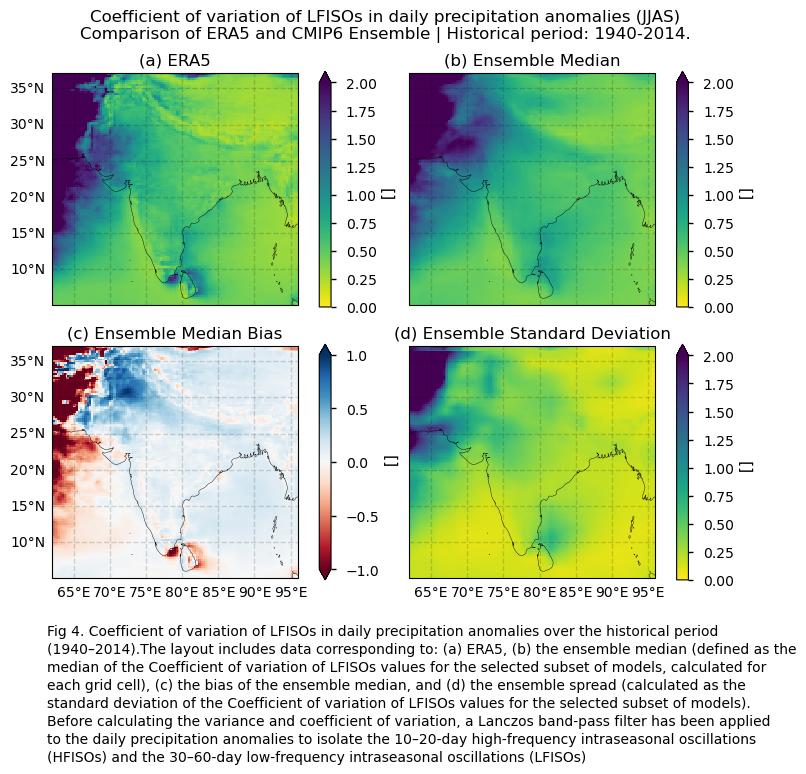
Maps showing the spatial distribution of the variance of filtered daily precipitation anomalies, calculated for the historical period 1940–2014. The results compare ERA5 and the ensemble median, defined as the median of the variance values for the selected subset of models, calculated for each grid cell. The layout includes ERA5, the ensemble median, the ensemble median bias, and the ensemble spread (derived as the standard deviation of the variance for the selected subset of models). The same layout is displayed for the coefficient of variation.
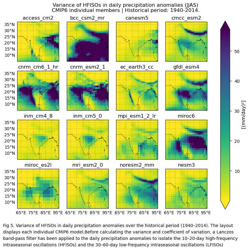
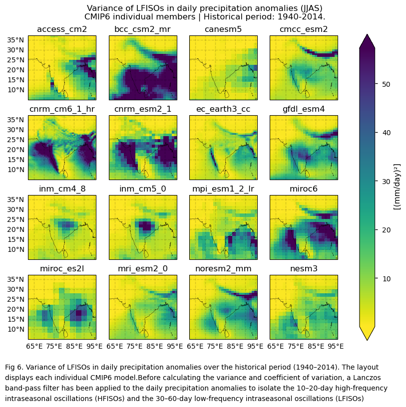
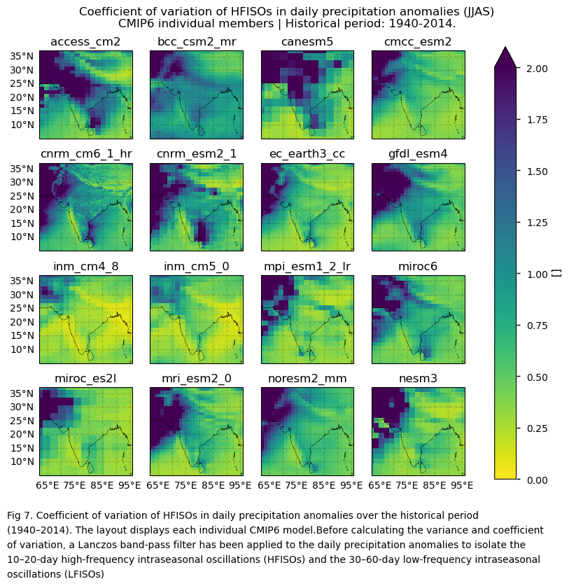
Maps showing the spatial distribution of the variance of filtered daily precipitation anomalies, calculated for the historical period 1940–2014 for each model. The same layout is displayed for the coefficient of variation.
Bias maps of the variance of filtered daily precipitation anomalies, calculated for the historical period 1940–2014 for each model. The same layout is displayed for the coefficient of variation.
Time series showing the evolution of the 30-year variance and coefficient of variation (standard deviation divided by the mean) of filtered daily precipitation anomalies over the historical period, including trends and inter-model spread.

Note: A Lanczos band-pass filter is applied to isolate the 10–20-day (HFISOs) and 30–60-day (LFISOs) components of daily precipitation anomalies. The seasonal period is JJAS.

3.1. Define plotting functions#

The functions presented here are used to plot layouts of the variance and coefficient of variation of filtered daily precipitation anomalies over the whole historical period.

Three layout types can be displayed, depending on the chosen function:

Layout including the reference ERA5 product, the ensemble median, the bias of the ensemble median, and the ensemble spread: plot_ensemble() is used.
Layout including every model: plot_models() is employed.
Layout including the bias of every model: plot_models() is used again.

Show code cell source Hide code cell source

#Define function to plot the caption of the figures (for the ensmble case)
def add_caption_ensemble(exp, mode_var="Variance"):

    caption_text= (
            f"Fig {fig_number}. {mode_var} in daily precipitation anomalies "
            f"over the {exp} period ({year_start}–{year_stop})."
            f"The layout includes data corresponding to: (a) ERA5, (b) the ensemble median "
            f"(defined as the median of the {mode_var} values for the selected "
            f"subset of models, calculated for each grid cell), "
            f"(c) the bias of the ensemble median, and (d) the ensemble spread "
            f"(calculated as the standard deviation of the {mode_var} values "
            f"for the selected subset of models). Before calculating the variance and coefficient of variation, "
            f"a Lanczos band-pass filter has been applied to the daily precipitation anomalies to isolate the " 
            f"10–20-day high-frequency intraseasonal oscillations (HFISOs) and the 30–60-day low-frequency "
            f"intraseasonal oscillations (LFISOs)"
    )

            
    wrapped_lines = textwrap.wrap(caption_text, width=105)
    # Add each line to the figure
    for i, line in enumerate(wrapped_lines):
        fig.text(0.05, -0.05  - i * 0.03, line, ha='left', fontsize=10)
    #end captioning


#Define function to plot the caption of the figures (for the individual models case)
def add_caption_models(bias,exp, mode_var="Variance"):
    #Add caption to the figure
    if bias: 
        caption_text = (
                f"Fig {fig_number}. Bias of the {mode_var} in daily precipitation anomalies "
                f"over the {exp} period ({year_start}–{year_stop}). "
                f"The layout displays each "
                f"individual {collection_id} model. Before calculating the variance and coefficient of variation, "
                f"a Lanczos band-pass filter has been applied to the daily precipitation anomalies to isolate the " 
                f"10–20-day high-frequency intraseasonal oscillations (HFISOs) and the 30–60-day low-frequency "
                f"intraseasonal oscillations (LFISOs)"
        )
    else:       
        caption_text = (
                f"Fig {fig_number}. {mode_var} in daily precipitation anomalies "
                f"over the {exp} period ({year_start}–{year_stop}). "
                f"The layout displays each individual "
                f"{collection_id} model.Before calculating the variance and coefficient of variation, "
                f"a Lanczos band-pass filter has been applied to the daily precipitation anomalies to isolate the " 
                f"10–20-day high-frequency intraseasonal oscillations (HFISOs) and the 30–60-day low-frequency "
                f"intraseasonal oscillations (LFISOs)"
        )

    wrapped_lines = textwrap.wrap(caption_text, width=110)
    # Add each line to the figure
    for i, line in enumerate(wrapped_lines):
        fig.text(0, -0.05  - i * 0.03, line, ha='left', fontsize=10)

def set_extent(da, axs, area):
    extent = [area[i] for i in (1, 3, 2, 0)]
    for i, coord in enumerate(extent):
        extent[i] += -2 if i % 2 else +2
    for ax in axs:
        # Grid
        subplotspec = ax.get_subplotspec()
        gridliners = [a for a in ax.artists if isinstance(a, Gridliner)]
        for gl in gridliners:
            gl.remove()
            gl = ax.gridlines(draw_labels=True, linestyle="--", linewidth=1, color="black", alpha=0.15)
            gl.top_labels = gl.right_labels = False
            gl.left_labels = subplotspec.is_first_col()
            gl.bottom_labels = subplotspec.is_last_row()
        # Extent
        ax.set_extent(extent)

def plot_models(
    data,
    da_for_kwargs=None,
    col_wrap=4,
    subplot_kw={"projection": ccrs.PlateCarree()},
    figsize=None,
    layout="constrained",
    area=area,
    flip_cmaps=False,
    **kwargs,
):
    if isinstance(data, dict):
        assert da_for_kwargs is not None
        model_dataarrays = data
    else:
        da_for_kwargs = da_for_kwargs or data
        model_dataarrays = dict(data.groupby("model"))

    # Get kwargs
    default_kwargs = {"robust": True, "extend": "both"}
    kwargs = default_kwargs | kwargs
    kwargs = xr.plot.utils._determine_cmap_params(da_for_kwargs.values, **kwargs)

    fig, axs = plt.subplots(
        *(col_wrap, math.ceil(len(model_dataarrays) / col_wrap)),
        subplot_kw=subplot_kw,
        figsize=figsize,
        layout=layout,
    )
    axs = axs.flatten()
    for (model, da), ax in zip(model_dataarrays.items(), axs):
        pcm = plot.projected_map(
            da, ax=ax, show_stats=False, add_colorbar=False, **kwargs
        )
        ax.set_title(model)
    set_extent(da_for_kwargs, axs, area)
    fig.colorbar(
        pcm,
        ax=axs.flatten(),
        extend=kwargs["extend"],
        location="right",
        label=f"{da_for_kwargs.attrs.get('long_name', '')} [{da_for_kwargs.attrs.get('units', '')}]",
    )
    return fig




def plot_ensemble(
    da_models,
    da_era5=None,
    subplot_kw={"projection": ccrs.PlateCarree()},
    figsize=None,
    layout="constrained",
    cbar_kwargs=None,
    area=area,
    flip_cmaps=False,
    cmap_params_era5=None,
    cmap_params_median=None,
    cmap_params_bias=None,
    cmap_params_std=None,
    **kwargs,
):
    import matplotlib.pyplot as plt
    import xarray as xr

    # Default behaviour
    default_kwargs = {"robust": True, "extend": "both"}
    if da_era5 is None and cbar_kwargs is None:
        cbar_kwargs = {"orientation": "horizontal"}

    # Create figure and axes
    fig, axs = plt.subplots(
        *(1 if da_era5 is None else 2, 2),
        subplot_kw=subplot_kw,
        figsize=figsize,
        layout=layout,
    )
    axs = axs.flatten()
    axs_iter = iter(axs)

    # --- ERA5 plot ---
    if da_era5 is not None:
        ax = next(axs_iter)
        params = cmap_params_era5 or xr.plot.utils._determine_cmap_params(
            da_era5.values, **default_kwargs
        )
        plot.projected_map(
            da_era5, ax=ax, show_stats=False, cbar_kwargs=cbar_kwargs, **params
        )
        ax.set_title("(a) ERA5")

    # --- Ensemble Median ---
    ax = next(axs_iter)
    median = da_models.median("model", keep_attrs=True)
    params = cmap_params_median or xr.plot.utils._determine_cmap_params(
        da_era5.values, **default_kwargs
    )
    plot.projected_map(
        median, ax=ax, show_stats=False, cbar_kwargs=cbar_kwargs, **params
    )
    ax.set_title("(b) Ensemble Median" if da_era5 is not None else "(a) Ensemble Median")

    # --- Ensemble Bias (Median - ERA5) ---
    if da_era5 is not None:
        ax = next(axs_iter)
        with xr.set_options(keep_attrs=True):
            bias = median - da_era5
        params = cmap_params_bias or xr.plot.utils._determine_cmap_params(
            bias.values, center=0, **default_kwargs
        )
        plot.projected_map(
            bias,
            ax=ax,
            show_stats=False,
            cbar_kwargs=cbar_kwargs,
            **params,
        )
        ax.set_title("(c) Ensemble Median Bias")

    # --- Ensemble Standard Deviation ---
    ax = next(axs_iter)
    std = da_models.std("model", keep_attrs=True)
    params = cmap_params_std or xr.plot.utils._determine_cmap_params(
        std.values, **default_kwargs
    )
    plot.projected_map(
        std,
        ax=ax,
        show_stats=False,
        cbar_kwargs=cbar_kwargs,
        **params,
    )
    ax.set_title("(d) Ensemble Standard Deviation" if da_era5 is not None else "(b) Ensemble Standard Deviation")

    # Set extent
    set_extent(da_models, axs, area)

    return fig

3.2. Plot ensemble maps#

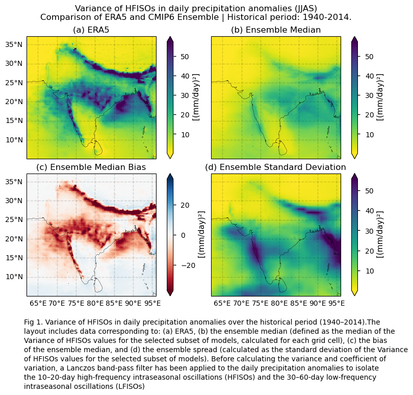
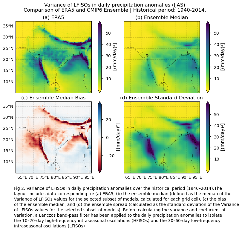
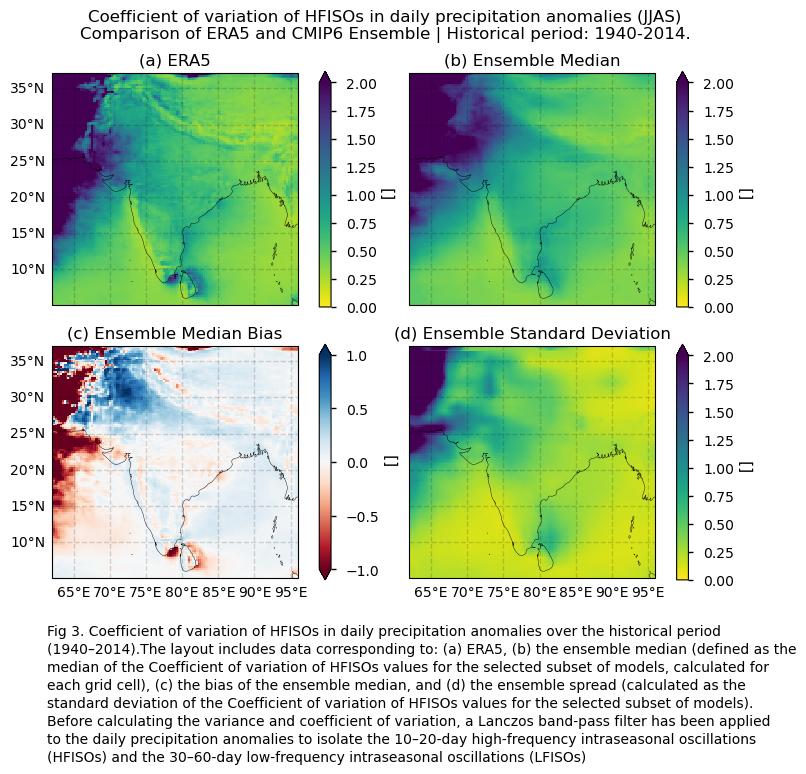
In this section, we invoke the plot_ensemble() function to visualise the variance values of filtered daily precipitation anomalies over the period 1940–2014 for the following: (a) the reference ERA5 product, (b) the ensemble median (defined as the median of the variance values for the selected subset of models, calculated for each grid cell), (c) the bias of the ensemble median, and (d) the ensemble spread (calculated as the standard deviation of the variance for the selected subset of models). The same layout of maps is displayed for the coefficient of variation. As mentioned throughout this notebook, before calculating the variance and coefficient of variation, a Lanczos band-pass filter has been applied to the daily precipitation anomalies to isolate the 10–20-day high-frequency intraseasonal oscillations (HFISOs) and the 30–60-day low-frequency intraseasonal oscillations (LFISOs).

../../_images/4ea689bc5c2bcef83f3c84dbd6729daf1f2fd2224885f5dedd1a48166e4cc569.png

../../_images/a62fd7ad2734cac1e5cc50af7b304816cc5e7729e0b25fe0bb06729dcaef1e92.png

../../_images/1df883f16aeeea583927f76f6a47a132199d105ae409a4bc6b36439777deabf2.png

../../_images/1fef48c1d95f4e61846b13b7832e375c474c6259108bac65c0560ec2835d32a2.png

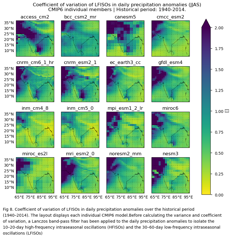
3.3. Plot model maps#

In this section, we invoke the plot_models() function to visualise the variance and the coefficient of variation of filtered daily precipitation anomalies over the period 1940–201, for every model individually. As mentioned throughout this notebook, before calculating the variance and coefficient of variation, a Lanczos band-pass filter has been applied to the daily precipitation anomalies to isolate the 10–20-day high-frequency intraseasonal oscillations (HFISOs) and the 30–60-day low-frequency intraseasonal oscillations (LFISOs). Note that the model data used in this section maintains its original grid.

../../_images/adb91441b452e18b914d4b48c1a7c0809e0f9ff6459d76cd271b9bee4d6cd6f4.png

../../_images/e15a6927991cba886faa039257cb84a24a120e197da8e519845d378ea02c1ad8.png

../../_images/8ff53a66064517b02e1f3062550b3c205544b05ba31e5841baa21975f31f645e.png

../../_images/4cf2d5288893124b5118c2c414697ed061437975ae1d2015f92e058a0abd03d7.png

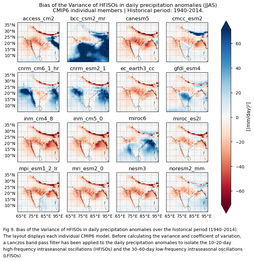
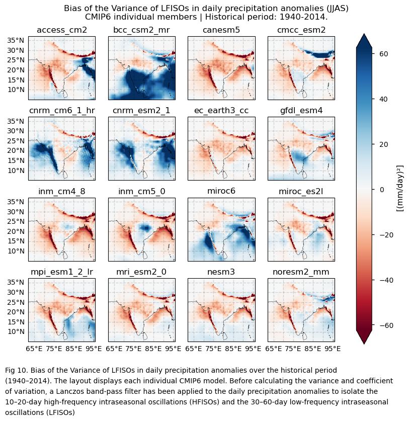
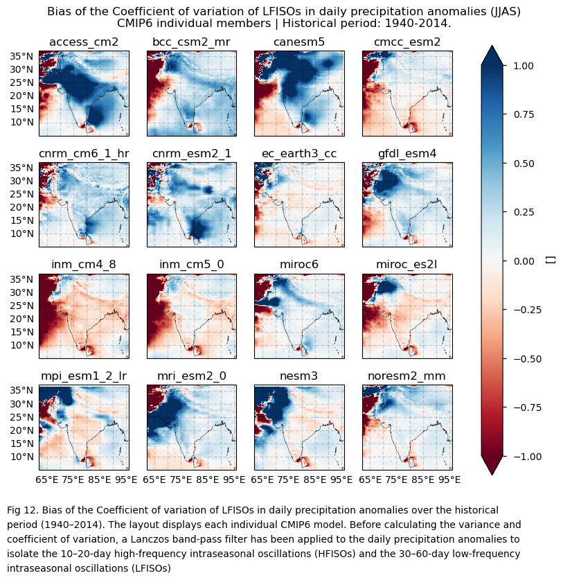
3.4. Plot bias maps#

In this section, we invoke the plot_models() function to visualise the bias of the variance and the coefficient of variation for filtered daily precipitation anomalies over the period 1940–2014, for every model individually. As mentioned throughout this notebook, before calculating the variance and coefficient of variation, a Lanczos band-pass filter has been applied to the daily precipitation anomalies to isolate the 10–20-day high-frequency intraseasonal oscillations (HFISOs) and the 30–60-day low-frequency intraseasonal oscillations (LFISOs). Note that the model data used in this section has previously been interpolated to the ERA5 grid.

../../_images/971e631d8207ae3356a3e4c8a1493edf9c9e45cce26b21947869fb654d576cfe.png

../../_images/c4118d2bef11e65c60afb1b15a2c32e1de58ce264e03d12c373a340856ab2f38.png

../../_images/c42b2d9577c67dcc20ad6a6d48df29d1329d72a1b85d11b0d6c289017c24003e.png

../../_images/eeb877df3dadc043a3f7e8319d0cb4ca42ceca71af21c67aaecc4a5f9a6ff1c8.png

3.5. Timeseries of the coefficient of variation#

This section examines the time series of spatially averaged variance and coefficient of variation, calculated from filtered daily precipitation anomalies over the historical period using a 30-year window. The analysis compares the CMIP6 ensemble median, ERA5, and individual models, highlighting trends for both the CMIP6 ensemble median and ERA5. It also displays the ensemble spread, along with the slope values of the trends for ERA5 and the CMIP6 ensemble median.

As mentioned throughout this notebook, before calculating the variance and coefficient of variation, a Lanczos band-pass filter has been applied to the daily precipitation anomalies to isolate the 10–20-day high-frequency intraseasonal oscillations (HFISOs) and the 30–60-day low-frequency intraseasonal oscillations (LFISOs).

Show code cell source Hide code cell source

# Define the colors
colors = {"CMIP6": "green", "ERA5": "black"}

# Cutout region
regionalise_kwargs = {
    "lon_slice": slice(area_timeseries[1], area_timeseries[3]),
    "lat_slice": slice(area_timeseries[0], area_timeseries[2]),
}

def plot_trend(time_series, var_values, label, color):
    time_numeric = pd.to_numeric(time_series.to_series())
    slope, intercept, _, p_value, _ = linregress(time_numeric, var_values)
    trend = intercept + slope * time_numeric
    slope_per_decade = slope * 10 * (60 * 60 * 24 * 365.25 * 10**9)  # nanoseconds to decade
    plt.plot(time_series, trend, linestyle='--', color=color, label=label)
    return slope_per_decade, p_value

for var in ["HFISOs_10_20_variance", "LFISOs_30_60_variance", "HFISOs_10_20_coefficient_of_variation", "LFISOs_30_60_coefficient_of_variation"]:
    # Get the spatial mean for ERA5
    era5_mean = diagnostics.spatial_weighted_mean(utils.regionalise(ds_era5, **regionalise_kwargs))[var]

    # Get the spatial mean for CMIP6, preserving each model
    cmip6_means = [
        diagnostics.spatial_weighted_mean(
            utils.regionalise(ds.expand_dims(model=[model]), **regionalise_kwargs)
        )[var] for model, ds in model_datasets.items()
    ]

    # Calculate the median, ensemble mean, and standard deviation
    cmip6_mean_median = xr.concat(cmip6_means, dim="model").median("model", keep_attrs=True)
    cmip6_mean_ens_mean = xr.concat(cmip6_means, dim="model").mean("model", keep_attrs=True)
    cmip6_mean_std = xr.concat(cmip6_means, dim="model").std("model", keep_attrs=True)

    # Initialize list to store trend information
    trend_info = []

    era5_var = era5_mean.sel(variance=variance_window[0])
    cmip6_var = cmip6_mean_median.sel(variance=variance_window[0])
    cmip6_var_ens_mean = cmip6_mean_ens_mean.sel(variance=variance_window[0])
    cmip6_mean_std_sel = cmip6_mean_std.sel(variance=variance_window[0])
            
    # Plotting
    plt.figure(figsize=(10, 5))

    # Plot individual model series for each variance
    for model_data in cmip6_means:
        model_var = model_data.sel(variance=variance_window[0])
        model_var_values = model_var.values.flatten() if model_var.ndim > 1 else model_var.values
        plt.plot(model_var['time'], model_var_values, linestyle='-', color="grey", alpha=0.3)

    plt.plot([], [], linestyle='-', color='grey', alpha=0.3, label='Individual Models')

    era5_var.plot(label=f"ERA5", color=colors["ERA5"])
    cmip6_var.plot(label=f"CMIP6", color=colors["CMIP6"])

    plt.fill_between(
        cmip6_var_ens_mean['time'],
        cmip6_var_ens_mean.values + cmip6_mean_std_sel,
        cmip6_var_ens_mean.values - cmip6_mean_std_sel,
        color=colors["CMIP6"], alpha=0.2, label=f'CMIP6 Spread'
    )

    slope_era5, p_value_era5 = plot_trend(era5_var['time'][~np.isnan(era5_var.values)],
                                          era5_var.values[~np.isnan(era5_var.values)], 
                                          f"ERA5 Trend", colors["ERA5"])

    slope_cmip6, p_value_cmip6 = plot_trend(cmip6_var['time'][~np.isnan(cmip6_var.values)],
                                            cmip6_var.values[~np.isnan(cmip6_var.values)], 
                                            f"CMIP6 Median Trend", colors["CMIP6"])

    trend_info = [
        (f"ERA5 {variance_window[0]}-year {mode_var_string[var]}", slope_era5, p_value_era5),
        (f"CMIP6 Median {variance_window[0]}-year {mode_var_string[var]}", slope_cmip6, p_value_cmip6)
    ]

    plt.xlabel('End year of the moving window')
    string_freq = f"(from {timeseries} {cmip6_variable_short} means)"
    title_numb = "(a)" if var == "HFISOs_10_20_variance" else \
             "(b)" if var == "LFISOs_30_60_variance" else \
             "(c)" if var == "HFISOs_10_20_coefficient_of_variation" else \
             "(d)"
    plt.title(
        f"{title_numb} {mode_var_string[var]} in daily precipitation anomalies . "
        f"Width of the moving window: {variance_window[0]}-year. \n"
        f"Region: lon [{area_timeseries[1]}E, {area_timeseries[3]}E] x lat [{area_timeseries[2]}N, {area_timeseries[0]}N] \n"
        f"Period: {year_start}-{year_stop}. Season: {timeseries}"
    )

    plt.legend()
    plt.grid()
    ax = plt.gca()
    ax.xaxis.set_major_formatter(mdates.DateFormatter('%Y'))
    plt.gcf().autofmt_xdate()

    units = "(mm/day)²" if var in ["LFISOs_30_60_variance","HFISOs_10_20_variance"] else ""
    plt.ylabel(f"{units}")
    units = "(mm/day)²" if var in ["LFISOs_30_60_variance","HFISOs_10_20_variance"] else "1"
    plt.gcf().text(0.13, -0.015,
                    '\n'.join([f"{name} Trend: {trend:.4f} ({units}/decade), p-value: {p:.3e}"
                                for name, trend, p in trend_info]),
                    fontsize=12,
                    ha='left', va='center',
                    bbox=dict(boxstyle="square,pad=0.5", edgecolor="black", facecolor="lightgray"))

    plt.ylim((0.45, 1.0) if var in ["HFISOs_10_20_coefficient_of_variation", "LFISOs_30_60_coefficient_of_variation"] else (0,40))
    plt.show()
    print(f"\n")

../../_images/7d48e83295b1503d3e529b4716da9034937c4d59e4e7f88dcabd973462dc6aae.png

../../_images/5e2ebed9ea53018556d7019b117a4c8b625c83e351cad0f34b8fdc21c1bb1f8a.png

../../_images/a42dc77dc21959125e81adfae17b8de6a0ff2fdbc5a6cf96673d809ad5adf5a4.png

../../_images/8f1f255d120ccc589384e96e0c62ff4340d7aa25786b21e69da809c3d73299f2.png

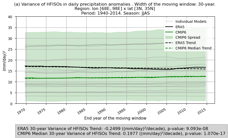
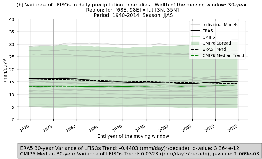
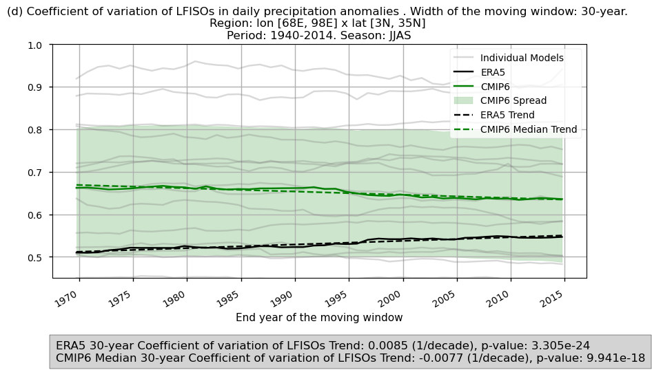
Fig 13. Time series of the spatially averaged values for the chosen variability formulations: (a) variance and (b) coefficient of variation, for filtered daily precipitation anomalies over the period 1940–2014. The variance and coefficient of variation have been calculated using a 30-year window. Each time series displays the CMIP6 ensemble median (green), ERA5 (black), and individual models (grey), with dashed lines indicating the trend for the CMIP6 ensemble median and ERA5. The shaded area represents the ensemble spread. A grey box at the bottom displays the trend slope. Before calculating the variance and coefficient of variation, a Lanczos band-pass filter has been applied to the daily precipitation anomalies to isolate the 10–20-day high-frequency intraseasonal oscillations (HFISOs) and the 30–60-day low-frequency intraseasonal oscillations (LFISOs).

3.6. Results summary and discussion#

An assessment evaluating the capability of CMIP6 GCMs to represent inter-annual precipitation variability complements the results presented in this notebook.
Intra-seasonal variability during the Monsoon season (JJAS) shows substantial differences in spatial patterns depending on the formulation used—variance or the coefficient of variation (standard deviation divided by the mean). As detailed throughout, a Lanczos band-pass filter is applied to daily precipitation anomalies to isolate 10–20-day high-frequency (HFISOs) and 30–60-day low-frequency (LFISOs) oscillations. Anomalies are computed relative to the daily climatology to remove the seasonal cycle.
Using variance to assess inter-annual variability reveals large differences in bias sign, magnitude, and spatial distribution. Despite model differences, biases are consistently influenced by orography and high-precipitation regions. These regions show high absolute biases due to high JJAS precipitation, though not necessarily large relative to the mean. The coefficient of variation (CV) normalises this effect, offering a potentially more meaningful measure of variability—though it can yield high values where climatological means are near zero.
Differences between models are smaller when using CV compared to variance. Inland north-western regions (with near-zero or very low seasonal averages) show strong negative biases and high inter-model spread. One hypothesis to explain this may be that unusually wet spells are underestimated in comparison to ERA5.
The spatial patterns of variance and CV for HFISOs and LFISOs are largely similar.
Intra-seasonal variability patterns strongly resemble those seen in the inter-annual assessment, suggesting intra-seasonal timescales may influence inter-annual variability [10].
CMIP6 ensemble median does not accurately capture the temporal evolution of variance and coefficient of variation in filtered daily anomalies averaged over India (HFISOs and LFISOs). While ERA5 shows a decreasing trend in variance and increasing trend in coefficient of variation, CMIP6 models indicate opposite trends, highlighting discrepancies in temporal representation. The trends for the selection region are statistically significant with p-values below 0.05.

3.7. Implications for the users#

The selection of the variability formulation matters. The Coefficient of Variation (CV) reduces orographic influence by normalising variability by the mean, and shows smaller inter-model differences than variance. However, it can produce artefactually high values in north-western inland regions where mean precipitation is very low.
ERA5 has biases [13][14]. While ERA5 is used for its temporal coverage, it has known biases. Users may consider alternative references like the GPCP dataset, which may yield different results.
Unlike the inter-annual assessment, CV and variance show opposite trends over time. ERA5 indicates a decline in variance and a rise in the coefficient of variation, while CMIP6 models show the reverse.
It is important to consider a larger ensemble and acknowledge that the time series in this assessment represent spatially averaged values, which may lead to different results when focusing on specific sub-regions.
Frequency component consistency: No significant differences are seen in the spatial or temporal patterns between the low-frequency (LFISOs) and high-frequency (HFISOs) components of intra-seasonal oscillations.
Given the challenges in replicating the spatial patterns of variance and the coefficient of variation, as well as the difficulties in capturing their temporal evolution, bias correction of CMIP6 projections may be essential for effectively using future projections of intra-seasonal precipitation variability. Such improvements could facilitate the adoption of CMIP6 future projections in the water management sector, aiding in the design of strategies to adapt to projected changes in precipitation.
Intra-seasonal and inter-annual links. The spatial patterns of intra-seasonal variability closely resemble those found in the inter-annual variability assessment. Intra-seasonal variability may influence inter-annual variability [10] and, therefore, it may be important to bias correct data at the daily timescale.
Assessments using regional climate models (RCMs) may produce different results (not necessarily better) due to their higher spatial resolution, better representation of local processes, and more detailed treatment of orography and land-atmosphere interactions.

RESULTS NOTE:
It is important to note that the results presented are specific to the 16 models chosen, and users should aim to assess as wide a range of models as possible before making a sub-selection.

ℹ️ If you want to know more#

Key resources#

Some key resources and further reading were linked throughout this assessment.

The CDS catalogue entries for the data used were:

CMIP6 climate projections (Daily - Precipitation): https://cds.climate.copernicus.eu/datasets/projections-cmip6?tab=overview
ERA5 hourly data on single levels from 1940 to present (total precipitation): https://cds.climate.copernicus.eu/datasets/reanalysis-era5-single-levels?tab=overview

Code libraries used:

C3S EQC custom functions, c3s_eqc_automatic_quality_control, prepared by B-Open

References#

[1] Thornton, P. K., Ericksen, P. J., Herrero, M., and Challinor, A. J., 2014. Climate variability and vulnerability to climate change: A review. Global Change Biol. 20, https://doi.org/10.1111/gcb.12581

[2] Masroor, M., Rehman, S., Avtar, R., Sahana, M., Ahmed, R., Sajjad, H., 2020. Exploring climate variability and its impact on drought occurrence: evidence from Godavari Middle sub-basin, India. Weather and Climate Extremes. 30, 100277. https://doi.org/10.1016/j.wace.2020.100277

[3] Krishnamurti, T. N. and Ardanuy, P., 1980. 10 to 20-day westward propagating mode and “breaks in the monsoons”. Tellus, 32, 15–26. https://doi.org/10.1111/j.2153-3490.1980.tb01717.x

[4] Wen, M. and Zhang, R., 2007. Role of the quasi-biweekly oscillation in the onset of convection over the Indochina Peninsula, Q. J. R. Meteor. Soc., 133, 433–444. https://doi.org/10.1002/qj.38

[5] Wen, M., Yang, S., Higgins, R. W., Zhang, R., 2011. Characteristics of the dominant modes of atmospheric quasi-biweekly oscillation over tropical-subtropical Americas, J. Climate, 24, 3956–3970. https://doi.org/10.1175/2011JCLI3916.1

[6] Madden, R. A. and Julian P. R., 1971. Detection of a 40–50 day oscillation in the zonal wind in the tropical Pacific, J. Atmos. Sci., 28, 702–708. https://doi.org/10.1175/1520-0469(1971)028<0702:DOADOI>2.0.CO;2

[7] Madden, R. A. and Julian P. R., 1972. Description of global scale circulation cells in the tropics with 40–50 day period, J. Atmos. Sci., 29, 1109–1123. https://doi.org/10.1175/1520-0469(1972)029<1109:DOGSCC>2.0.CO;2

[8] Liu, F., Wang, B., Ouyang, Y., Wang, H., Qiao,S., Chen, G., Dong, W., 2022. Intraseasonal variability of global land monsoon precipitation and its recent trend. npj Clim Atmos Sci 5, 30. https://doi.org/10.1038/s41612-022-00253-7

[9], Jia, X. and Yang, S., 2013. Impact of the quasi-biweekly oscillation over the western North Pacific on East Asian subtropical monsoon during early summer, J. Geophys. Res. Atmos., 118, 4421–4434, https://doi.org/10.1002/jgrd.50422

[10] Jiang, X. and Ting, M., 2019. Intraseasonal Variability of Rainfall and Its Effect on Interannual Variability across the Indian Subcontinent and the Tibetan Plateau. J. Climate, 32, 2227–2245, https://doi.org/10.1175/JCLI-D-18-0319.1.

[11] Hatsuzuka, D., and Fujinami, H., 2017. Effects of the South Asian Monsoon Intraseasonal Modes on Genesis of Low Pressure Systems over Bangladesh. J. Climate, 30, 2481–2499, https://doi.org/10.1175/JCLI-D-16-0360.1.

[12] Yan, X., Yang, S., Wang, T., Maloney, E.D., Dong, S., Wei, W., He, S., 2019. Quasi-biweekly oscillation of the Asian monsoon rainfall in late summer and autumn: different types of structure and propagation. Clim Dyn 53, 6611–6628. https://doi.org/10.1007/s00382-019-04946-3

[13] Ramon, J., Lledó L., Torralba, V., Soret, A., Doblas-Reyes, F.J., 2019. What global reanalysis best represents near-surface winds?. Q J R Meteorol Soc. 2019; 145: 3236–3251. https://doi.org/10.1002/qj.3616

[14] Hassler, B., and Lauer, A., 2021. Comparison of Reanalysis and Observational Precipitation Datasets Including ERA5 and WFDE5. Atmosphere, 12, 1462. https://doi.org/10.3390/atmos12111462

Testing the capability of CMIP6 GCMs to represent precipitation intra-seasonal variability

Contents

5.1.1. Testing the capability of CMIP6 GCMs to represent precipitation intra-seasonal variability#

🌍 Use case: Assessing the potential impacts of climate change on precipitation variability over India#

❓ Quality assessment question#

📢 Quality assessment statement#

📋 Methodology#

📈 Analysis and results#

1. Parameters, requests and functions definition#

1.1. Import packages#

1.2. Define Parameters#

1.3. Define input models and output parameters#

1.4. Define ERA5 request#

1.5. Define model requests#

1.6. Functions to cache#

2. Downloading and processing#

2.1. Download and transform ERA5#

2.2. Download and transform models#

2.3. Change some attributes#

3. Plot and describe results#

3.1. Define plotting functions#

3.2. Plot ensemble maps#

3.3. Plot model maps#

3.4. Plot bias maps#

3.5. Timeseries of the coefficient of variation#

3.6. Results summary and discussion#

3.7. Implications for the users#

ℹ️ If you want to know more#

Key resources#

References#