Testing the capability of CMIP6 GCMs to represent precipitation variability

5.1.9. Testing the capability of CMIP6 GCMs to represent precipitation variability#

Production date: 19-01-2025

Produced by: CMCC foundation - Euro-Mediterranean Center on Climate Change. Albert Martinez Boti.

Most research has focused on projected long-term changes in mean climate and extremes, while changes in variability have received less attention. However, understanding the evolution of precipitation variability is crucial for accurately modelling climate phenomena and quantify climate change impacts, particularly on water resources and related socioeconomic factors [1],[2]. This notebook evaluates the capability of a subset of 16 CMIP6 Global Climate Models (GCMs) to represent inter-annual variability in seasonal mean precipitation over the Indian subcontinent, employing variance and the coefficient of variation (standard deviation divided by the mean) as measures of variability.

Systematic errors are assessed by comparing model outputs against the ERA5 reanalysis, which serves as the reference dataset. The analysis focuses on JJAS (June, July, August and September), traditionally regarded as the Indian Summer Monsoon period, though the methodology is adaptable for annual or other seasonal analyses. Spatial patterns of the variance and the coefficient of variation are examined for JJAS mean precipitation over the historical period from 1940 to 2014. Additionally, the temporal evolution of the spatially-averaged variance and coefficient of variation, including trends, is analysed using a 30-year moving window and presented as time series.

The analyses presented in this notebook provide valuable insights into the reliability of a subset of CMIP6 models in capturing precipitation inter-annual variability. Understanding the performance of these models can help the water management sector to make more informed decisions and supports the use of CMIP6 Global Climate Models (GCMs) in designing strategies to adapt to projected changes in variability.

🌍 Use case: Assessing the potential impacts of climate change on precipitation inter-annual variability over India for water management#

❓ Quality assessment question#

How well do CMIP6 projections represent historic inter-annual variability of precipitation across the Indian sub-continent? Are there trends affecting precipitation inter-annual variability?

📢 Quality assessment statement#

These are the key outcomes of this assessment

The choice of variability formulation is crucial when describing inter-annual variability during the summer Monsoon. The two formulations considered within this assessment reveal distinct spatial patterns.
Variance analyses reveal model-dependent differences in bias magnitude, sign, and spatial distribution. Despite these variations, all models show strong links to orography and high-precipitation regions, where biases remain significant due to high precipitation, even though they are not necessarily large relative to the mean. The coefficient of variation removes this effect by normalising the standard deviation (i.e., the square root of the variance) by the mean.
Model differences are less pronounced for the coefficient of variation than for variance. Most models underestimate it in the inland north-west, where seasonal mean precipitation is very low or near zero.
The 30-year time series of spatially averaged variance and coefficient of variation show a decreasing trend for ERA5, suggesting a decline in inter-annual variability over the historical period. This is evident from both variance magnitude—potentially influenced by the mean’s decline [3]—and the coefficient of variation, which removes the effect of the mean. However, the CMIP6 ensemble median for the subset of considered models shows the opposite trend.
Understanding and correcting the biases of CMIP6 projections of precipitation variability may increase confidence when analysing projections assessing the future inter-annual variability which can help on planning for water resource allocation, flood mitigation, and agricultural management, ensuring resilience against the challenges posed by a changing climate.

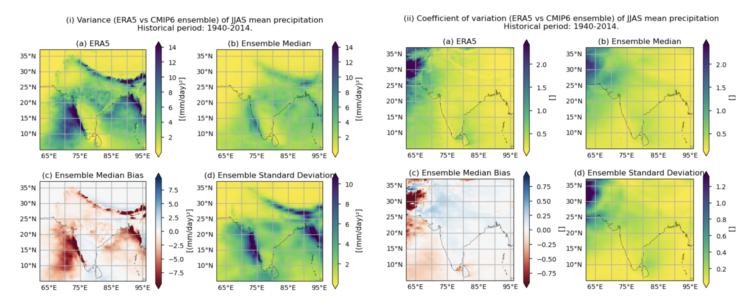
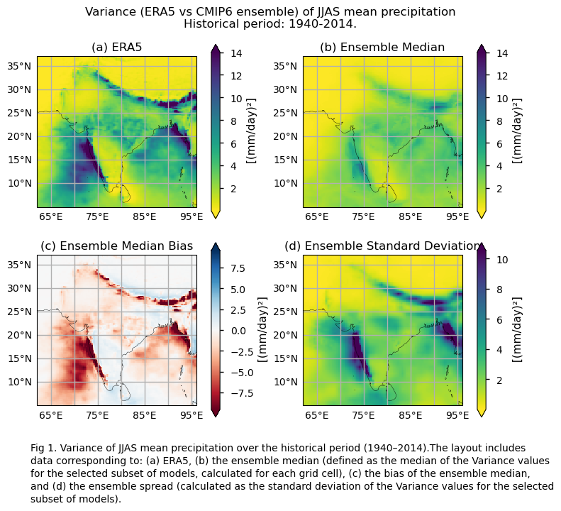
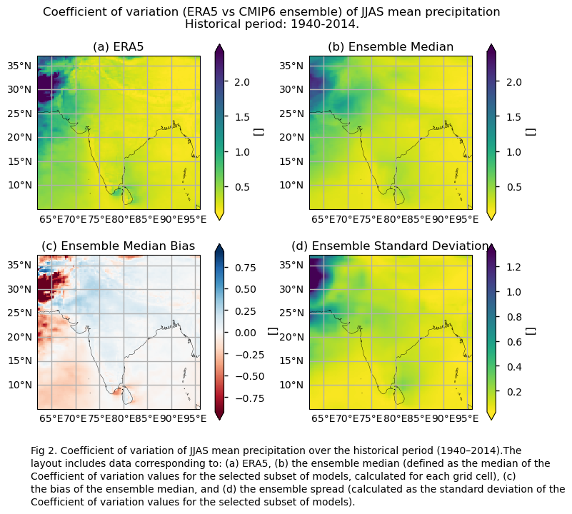
Mean Bias variance — Fig. 5.1.9.1 Fig A. i. Variance of JJAS mean precipitation over the historical period (1940–2014). The layout includes data corresponding to: (a) ERA5, (b) the ensemble median (defined as the median of the variance values for the selected subset of models, calculated for each grid cell), (c) the bias of the ensemble median, and (d) the ensemble spread (calculated as the standard deviation of the variance values for the selected subset of models). Fig A.ii. Same as Fig. A.i. but for the coefficient of variation.#

📋 Methodology#

A subset of 16 models from the CMIP6 project is used to calculate the variance and the coefficient of variation (standard deviation divided by the mean), which serve as formulations to characterise precipitation inter-annual variability in this notebook. Spatial patterns of variance and the coefficient of variation for seasonal mean precipitation, along with their associated biases (using ERA5 as reference), are displayed for each model and the ensemble median (per grid cell). Additionally, the spatially averaged temporal evolution of the variance and coefficient of variation, including trends, is analysed using a 30-year moving window and presented as time series, following a methodology similar to [4].

The analysis focuses on the Indian subcontinent during the historical period from 1940 to 2014 and examines the JJAS period, traditionally regarded as the Indian Summer Monsoon (or rainy) season, although the methodology can be adapted for other seasonal or annual periods.

The analysis and results follow the next outline:

1. Parameters, requests and functions definition

1.1. Import packages
1.2. Define Parameters
1.3. Define models
1.4. Define ERA5 request
1.5. Define model requests
1.6. Functions to cache

2. Downloading and processing

2.1. Download and transform ERA5
2.2. Download and transform models
2.3. Change some attributes

3. Plot and describe results

3.1. Define plotting functions
3.2. Plot ensemble maps
3.3. Plot model maps
3.4. Plot bias maps
3.5. Timeseries of the coefficient of variation
3.6. Results summary and discussion

📈 Analysis and results#

1. Parameters, requests and functions definition#

1.1. Import packages#

1.2. Define Parameters#

In the “Define Parameters” section, various customisable options for the notebook are specified:

The initial and ending year used for the historical period can be specified by changing the parameters year_start and year_stop (1940-2014 is chosen).
The timeseries set the temporal period. For instance, selecting “JJAS” implies considering only the June, July, August, September season.
area allows specifying the geographical domain of interest. A domain including the Indian sub-continent has been selected.
The interpolation_method parameter allows selecting the interpolation method when regridding is performed.
The chunk selection allows the user to define if dividing into chunks when downloading the data on their local machine. Although it does not significantly affect the analysis, it is recommended to keep the default value for optimal performance.
variable and collection_id are not customisable for this assessment and are set to ‘precipitation’ and ‘CMIP6’. Expert users can use this notebook as a guide to create similar analyses for other variables or model sets (such as CORDEX).

1.3. Define models#

The following climate analyses are performed considering a subset of GCMs from CMIP6.

The selected CMIP6 models have available both the historical and SSP5-8.5 experiments.

1.4. Define ERA5 request#

Within this notebook, ERA5 serves as the reference product. In this section, we set the required parameters for the cds-api data-request of ERA5.

1.5. Define model requests#

In this section we set the required parameters for the cds-api data-request.

1.6. Functions to cache#

In this section, functions that will be executed in the caching phase are defined. Caching is the process of storing copies of files in a temporary storage location, so that they can be accessed more quickly. This process also checks if the user has already downloaded a file, avoiding redundant downloads.

Functions description:

get_grid_out and add_bounds ensure the regrid is performed properly.
The select_timeseries function subsets the dataset based on the chosen timeseries parameter.
The compute_rolling_variance function calculates the rolling variance and coefficient of variation using a 30-year window (which are needed when displaying the time series afterwards). It also computes the variance and coefficient of variation for the entire period.
The compute_interannual_variance function selects the season using the select_timeseries function. It then computes the rolling variance (and coefficient of variation) over the historical period (1940–2014) by calling compute_rolling_variance. The window width is 30 years, with a step size of one year. The variance and coefficient of variation is also calculated for the whole historical period.

Show code cell source Hide code cell source

def get_month_info(season_abbreviation):
    season_to_month = {
        "DJF": ("DEC", 12, "12", "02"),
        "MAM": ("MAR", 3, "03", "05"),
        "JJA": ("JUN", 6, "06", "08"),
        "SON": ("SEP", 9, "09", "11"),
        "JJAS":("JUN", 6, "06", "09"),    
    }
    return season_to_month.get(season_abbreviation)

def select_timeseries(ds, timeseries, year_start, year_stop):
    if timeseries == "annual":
        return ds.sel(time=slice(str(year_start), str(year_stop)))
    ds=ds.sel(time=slice(f"{year_start}-{get_month_info(timeseries)[2]}",
                         f"{year_stop}-{get_month_info(timeseries)[3]}"))
    return ds

def compute_rolling_variance(ds, window_years):
    (da,) = ds.data_vars.values()
    var = da.rolling(time=window_years, center=False).var()
    coeff=(var**(1/2))/da.rolling(time=window_years, center=False).mean()
    ds = xr.merge([var, coeff.rename("coefficient_of_variation")])
    return ds.expand_dims(variance=[window_years])

def add_bounds(ds):
    for coord in {"latitude", "longitude"} - set(ds.cf.bounds):
        ds = ds.cf.add_bounds(coord)
    return ds

def get_grid_out(request_grid_out, method):
    ds_regrid = download.download_and_transform(*request_grid_out)
    coords = ["latitude", "longitude"]
    if method == "conservative":
        ds_regrid = add_bounds(ds_regrid)
        for coord in list(coords):
            coords.extend(ds_regrid.cf.bounds[coord])
    grid_out = ds_regrid[coords]
    coords_to_drop = set(grid_out.coords) - set(coords) - set(grid_out.dims)
    return grid_out.reset_coords(coords_to_drop, drop=True)


def compute_interannual_variance(
    ds, timeseries, year_start, year_stop, variance_values,
    request_grid_out=None, **regrid_kwargs
):
    # Select the time series
    ds = select_timeseries(ds, timeseries, year_start, year_stop)
    
    # Get seasonal/annual means
    resampled = ds.resample(time="Y" if timeseries=="annual" else f"{len(timeseries)}MS")
    if timeseries=="annual":
        ds = getattr(resampled, "mean")(keep_attrs=True)
    else:
        ds = getattr(resampled, "mean")(keep_attrs=True).groupby('time.month')[get_month_info(timeseries)[1]]

    #Change units
    ds *=86400 
    
    # Compute variances
    datasets = [
        compute_rolling_variance(
            ds,
            window_years=variance)
        for variance in variance_values
    ]
    ds = xr.concat(datasets, "variance")

    # Handle grid output if requested
    if request_grid_out:
        grid_out = get_grid_out(request_grid_out, method=regrid_kwargs["method"])
        ds = diagnostics.regrid(ds, grid_out=grid_out, **regrid_kwargs)
    
    return ds.convert_calendar('proleptic_gregorian', align_on='date', use_cftime=False)

2. Downloading and processing#

2.1. Download and transform ERA5#

In this section, the download.download_and_transform function from the ‘c3s_eqc_automatic_quality_control’ package is used to download ERA5 reference monthly data, select the season (e.g., “JJAS” in this case) and compute the variance and coefficient of variation for the entire historical period, as well as for a 30-year rolling window. The results are then cached to prevent redundant downloads and processing.

2.2. Download and transform models#

In this section, the download.download_and_transform function from the ‘c3s_eqc_automatic_quality_control’ package is employed to download daily data from the CMIP6 models, select the season (“JJAS” in this example), compute the variance and coefficient of variation for the entire historical period, as well as for a 30-year rolling windows, interpolate to the ERA5 grid (only when specified; otherwise, the original model grid is maintained), and cache the results to avoid redundant downloads and processing.

model='access_cm2'
model='bcc_csm2_mr'
model='cmcc_esm2'
model='cnrm_cm6_1_hr'
model='cnrm_esm2_1'
model='ec_earth3_cc'
model='gfdl_esm4'
model='inm_cm4_8'
model='inm_cm5_0'
model='mpi_esm1_2_lr'
model='miroc6'
model='miroc_es2l'
model='mri_esm2_0'
model='noresm2_mm'
model='nesm3'
model='ukesm1_0_ll'

2.3. Change some attributes#

3. Plot and describe results#

This section will display the following results:

Maps showing the spatial distribution of the variance of JJAS mean precipitation calculated for the whole historical period 1940-2014 comparing ERA5 and the ensemble median (defined as the median of the variance values for the selected subset of models, calculated for each grid cell). The layout include ERA5, the ensemble median, the ensemble median bias and the ensemble spread (derived as the standard deviation of the variance for the selected subset of models). The same exact layout of maps is displayed for the coefficient of variation.
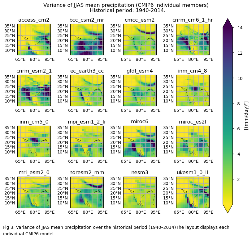
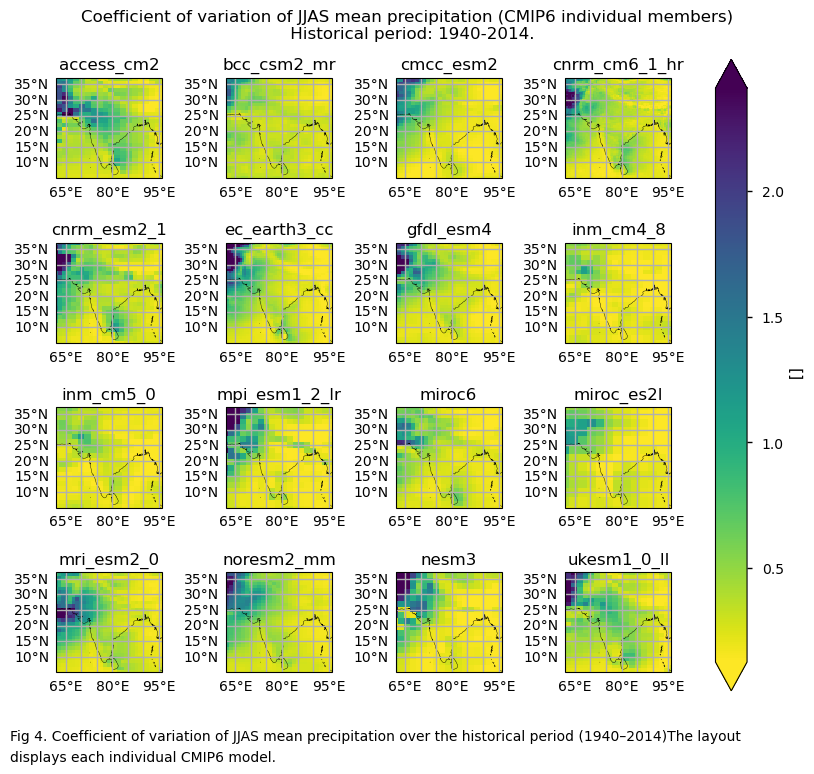
Maps showing the spatial distribution of the variance of JJAS mean precipitation calculated for the whole historical period 1940-2014 for each model. The same exact layout of maps is displayed for the coefficient of variation.
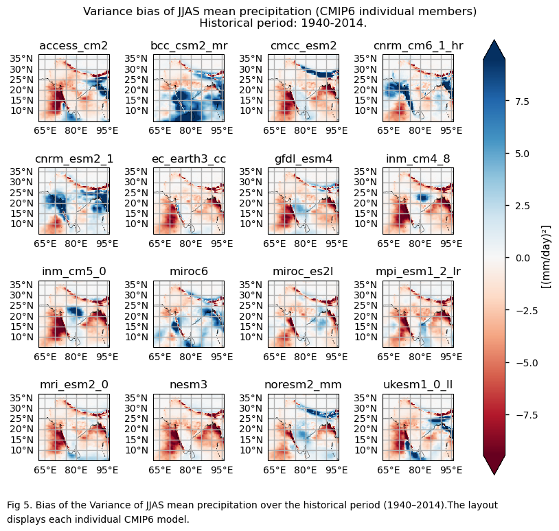
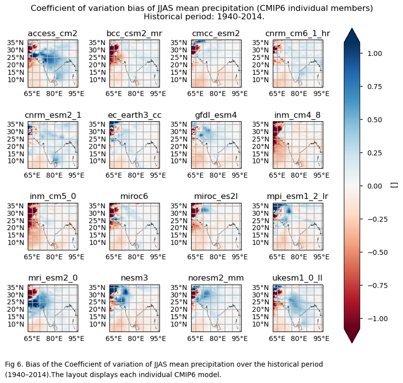
Bias maps of the variance and coefficient of variation of JJAS mean precipitation calculated for the whole historical period 1940–2014 for each model.
Timeseries showing the evolution of the 30-year variance and coefficient of variation (standard deviation divided by the mean) of JJAS mean precipitation over the historical period, including trends and inter-model spread.

3.1. Define plotting functions#

The functions presented here are used to plot layouts of the variance and coefficient of variation of seasonal mean precipitation over the whole historical period.

Three layout types can be displayed, depending on the chosen function:

Layout including the reference ERA5 product, the ensemble median, the bias of the ensemble median, and the ensemble spread: plot_ensemble() is used.
Layout including every model: plot_models() is employed.
Layout including the bias of every model: plot_models() is used again.

Show code cell source Hide code cell source

#Define function to plot the caption of the figures (for the ensmble case)
def add_caption_ensemble(exp, mode_var="Variance"):

    caption_text= (
            f"Fig {fig_number}. {mode_var} of "
            f"{timeseries} mean precipitation over the {exp} period ({year_start}–{year_stop})."
            f"The layout includes data corresponding to: (a) ERA5, (b) the ensemble median "
            f"(defined as the median of the {mode_var} values for the selected "
            f"subset of models, calculated for each grid cell), "
            f"(c) the bias of the ensemble median, and (d) the ensemble spread "
            f"(calculated as the standard deviation of the {mode_var} values "
            f"for the selected subset of models)."
    )
            
    wrapped_lines = textwrap.wrap(caption_text, width=105)
    # Add each line to the figure
    for i, line in enumerate(wrapped_lines):
        fig.text(0.05, -0.05  - i * 0.03, line, ha='left', fontsize=10)
    #end captioning


#Define function to plot the caption of the figures (for the individual models case)
def add_caption_models(bias,exp, mode_var="Variance"):
    #Add caption to the figure
    if bias: 
        caption_text = (
                f"Fig {fig_number}. Bias of the {mode_var} of "
                f"{timeseries} mean precipitation over the {exp} period ({year_start}–{year_stop})."
                f"The layout displays each "
                f"individual {collection_id} model."
        )
    else:       
        caption_text = (
                f"Fig {fig_number}. {mode_var} of "
                f"{timeseries} mean precipitation over the {exp} period ({year_start}–{year_stop})"
                f"The layout displays each individual "
                f"{collection_id} model."
        )

    wrapped_lines = textwrap.wrap(caption_text, width=110)
    # Add each line to the figure
    for i, line in enumerate(wrapped_lines):
        fig.text(0, -0.05  - i * 0.03, line, ha='left', fontsize=10)

def set_extent(da, axs, area):
    extent = [area[i] for i in (1, 3, 2, 0)]
    for i, coord in enumerate(extent):
        extent[i] += -2 if i % 2 else +2
    for ax in axs:
        ax.set_extent(extent)


def plot_models(
    data,
    da_for_kwargs=None,
    col_wrap=4,
    subplot_kw={"projection": ccrs.PlateCarree()},
    figsize=None,
    layout="constrained",
    area=area,
    flip_cmaps=False,
    **kwargs,
):
    if isinstance(data, dict):
        assert da_for_kwargs is not None
        model_dataarrays = data
    else:
        da_for_kwargs = da_for_kwargs or data
        model_dataarrays = dict(data.groupby("model"))

    # Get kwargs
    default_kwargs = {"robust": True, "extend": "both"}
    kwargs = default_kwargs | kwargs
    kwargs = xr.plot.utils._determine_cmap_params(da_for_kwargs.values, **kwargs)

    fig, axs = plt.subplots(
        *(col_wrap, math.ceil(len(model_dataarrays) / col_wrap)),
        subplot_kw=subplot_kw,
        figsize=figsize,
        layout=layout,
    )
    axs = axs.flatten()
    for (model, da), ax in zip(model_dataarrays.items(), axs):
        pcm = plot.projected_map(
            da, ax=ax, show_stats=False, add_colorbar=False, **kwargs
        )
        ax.set_title(model)
    set_extent(da_for_kwargs, axs, area)
    fig.colorbar(
        pcm,
        ax=axs.flatten(),
        extend=kwargs["extend"],
        location="right",
        label=f"{da_for_kwargs.attrs.get('long_name', '')} [{da_for_kwargs.attrs.get('units', '')}]",
    )
    return fig


def plot_ensemble(
    da_models,
    da_era5=None,
    subplot_kw={"projection": ccrs.PlateCarree()},
    figsize=None,
    layout="constrained",
    cbar_kwargs=None,
    area=area,
    flip_cmaps=False,
    **kwargs,
):
    # Get kwargs
    default_kwargs = {"robust": True, "extend": "both"}
    kwargs = default_kwargs | kwargs
    kwargs = xr.plot.utils._determine_cmap_params(
        da_models.values if da_era5 is None else da_era5.values, **kwargs
    )
    if da_era5 is None and cbar_kwargs is None:
        cbar_kwargs = {"orientation": "horizontal"}

    # Figure
    fig, axs = plt.subplots(
        *(1 if da_era5 is None else 2, 2),
        subplot_kw=subplot_kw,
        figsize=figsize,
        layout=layout,
    )
    axs = axs.flatten()
    axs_iter = iter(axs)

    # ERA5
    if da_era5 is not None:
        ax = next(axs_iter)
        plot.projected_map(
            da_era5, ax=ax, show_stats=False, cbar_kwargs=cbar_kwargs, **kwargs
        )
        ax.set_title("(a) ERA5")

    # Median
    ax = next(axs_iter)
    median = da_models.median("model", keep_attrs=True)
    plot.projected_map(
        median, ax=ax, show_stats=False, cbar_kwargs=cbar_kwargs, **kwargs
    )
    ax.set_title("(b) Ensemble Median" if da_era5 is not None else "(a) Ensemble Median")

    # Bias
    if da_era5 is not None:
        ax = next(axs_iter)
        with xr.set_options(keep_attrs=True):
            bias = median - da_era5
        plot.projected_map(
            bias,
            ax=ax,
            show_stats=False,
            center=0,
            cbar_kwargs=cbar_kwargs,
            **default_kwargs,
        )
        ax.set_title("(c) Ensemble Median Bias")

    # Std
    ax = next(axs_iter)
    std = da_models.std("model", keep_attrs=True)
    plot.projected_map(
        std, ax=ax, show_stats=False, cbar_kwargs=cbar_kwargs, **default_kwargs
    )
    ax.set_title("(d) Ensemble Standard Deviation" if da_era5 is not None else "(b) Ensemble Standard Deviation")

    set_extent(da_models, axs, area)
    return fig

3.2. Plot ensemble maps#

In this section, we invoke the plot_ensemble() function to visualise the variance values for JJAS mean precipitation over the period 1940–2014 for: (a) the reference ERA5 product, (b) the ensemble median (defined as the median of the variance values for the selected subset of models, calculated for each grid cell), (c) the bias of the ensemble median, and (d) the ensemble spread (calculated as the standard deviation of the variance for the selected subset of models). The same exact layout of maps is displayed for the coefficient of variation.

../../_images/b063c2be438f765011385f9d4923fafc20af44e5431ebac11b201c153a7aeada.png

../../_images/c7fcf857a8d5fe9b6e231f61dd1b006c3fb33fbaecc7224767697c212522888c.png

3.3. Plot model maps#

In this section, we invoke the plot_models() function to visualise the variance and the coefficient of variation of JJAS mean precipitation over the period 1940–2014 for every model individually. Note that the model data used in this section maintains its original grid.

../../_images/3bd98c8e50e2337c8ef49cc2b2dd14f3e87fcd6edccbded8760cc9151c53bbe5.png

../../_images/cd3570ec22b20d2355cda754ae41a58cb7e09abf033397f273e04019d719cc73.png

3.4. Plot bias maps#

In this section, we invoke the plot_models() function to visualise the bias of the variance and the coefficient of variation of JJAS mean precipitation over the period 1940–2014 for every model individually. Note that the model data used in this section has previously been interpolated to the ERA5 grid.

../../_images/fac5c70ec7e75a37029e8ea41ae94a0918d8a8cf7e80ff1afaa50f743950db87.png

../../_images/6e67330ca9e15bff187549df02d1bc5eadee505392bc140d23fd4d0cbae27d46.png

3.5. Timeseries of the coefficient of variation#

This section examines the time series of spatially averaged variance and coefficient of variation, calculated from JJAS mean precipitation over the historical period using a 30-year window. The analysis compares the CMIP6 ensemble median, ERA5, and individual models, highlighting trends for both the CMIP6 ensemble median and ERA5. It also displays the ensemble spread, along with the slope values of the trends for ERA5 and the CMIP6 ensemble median.

Show code cell source Hide code cell source

# Define the colors
colors = {"CMIP6": "green", "ERA5": "black"}

# Cutout region
regionalise_kwargs = {
    "lon_slice": slice(area[1], area[3]),
    "lat_slice": slice(area[0], area[2]),
}

def plot_trend(time_series, var_values, label, color):
    time_numeric = pd.to_numeric(time_series.to_series())
    slope, intercept, _, p_value, _ = linregress(time_numeric, var_values)
    trend = intercept + slope * time_numeric
    slope_per_decade = slope * 10 * (60 * 60 * 24 * 365.25 * 10**9)  # nanoseconds to decade
    plt.plot(time_series, trend, linestyle='--', color=color, label=label)
    return slope_per_decade, p_value

for var in ["pr", "coefficient_of_variation"]:
    # Get the spatial mean for ERA5
    era5_mean = diagnostics.spatial_weighted_mean(utils.regionalise(ds_era5, **regionalise_kwargs))[var]

    # Get the spatial mean for CMIP6, preserving each model
    cmip6_means = [
        diagnostics.spatial_weighted_mean(
            utils.regionalise(ds.expand_dims(model=[model]), **regionalise_kwargs)
        )[var] for model, ds in model_datasets.items()
    ]

    # Calculate the median, ensemble mean, and standard deviation
    cmip6_mean_median = xr.concat(cmip6_means, dim="model").median("model", keep_attrs=True)
    cmip6_mean_ens_mean = xr.concat(cmip6_means, dim="model").mean("model", keep_attrs=True)
    cmip6_mean_std = xr.concat(cmip6_means, dim="model").std("model", keep_attrs=True)

    # Initialize list to store trend information
    trend_info = []

    era5_var = era5_mean.sel(variance=variance_values[0])
    cmip6_var = cmip6_mean_median.sel(variance=variance_values[0])
    cmip6_var_ens_mean = cmip6_mean_ens_mean.sel(variance=variance_values[0])
    cmip6_mean_std_sel = cmip6_mean_std.sel(variance=variance_values[0])
            
    # Plotting
    plt.figure(figsize=(10, 5))

    # Plot individual model series for each variance
    for model_data in cmip6_means:
        model_var = model_data.sel(variance=variance_values[0])
        model_var_values = model_var.values.flatten() if model_var.ndim > 1 else model_var.values
        plt.plot(model_var['time'], model_var_values, linestyle='-', color="grey", alpha=0.3)

    plt.plot([], [], linestyle='-', color='grey', alpha=0.3, label='Individual Models')

    era5_var.plot(label=f"ERA5", color=colors["ERA5"])
    cmip6_var.plot(label=f"CMIP6", color=colors["CMIP6"])

    plt.fill_between(
        cmip6_var_ens_mean['time'],
        cmip6_var_ens_mean.values + cmip6_mean_std_sel,
        cmip6_var_ens_mean.values - cmip6_mean_std_sel,
        color=colors["CMIP6"], alpha=0.2, label=f'CMIP6 Spread'
    )

    slope_era5, p_value_era5 = plot_trend(era5_var['time'][~np.isnan(era5_var.values)],
                                          era5_var.values[~np.isnan(era5_var.values)], 
                                          f"ERA5 Trend", colors["ERA5"])

    slope_cmip6, p_value_cmip6 = plot_trend(cmip6_var['time'][~np.isnan(cmip6_var.values)],
                                            cmip6_var.values[~np.isnan(cmip6_var.values)], 
                                            f"CMIP6 Median Trend", colors["CMIP6"])

    trend_info = [
        (f"ERA5 {variance_values[0]}-year {mode_var_string[var]}", slope_era5, p_value_era5),
        (f"CMIP6 Median {variance_values[0]}-year {mode_var_string[var]}", slope_cmip6, p_value_cmip6)
    ]

    plt.xlabel('End year of the moving window')
    string_freq = f"(from {timeseries} {cmip6_variable_short} means)"
    title_numb="(a)" if var == "pr" else "(b)"
    plt.title(
        f"{title_numb} {mode_var_string[var]} {string_freq}. "
        f"Width of the moving window: {variance_values[0]}-year. \n"
        f"Region: lon [{area[1]}E, {area[3]}E] x lat [{area[2]}N, {area[0]}N] \n"
        f"Period: {year_start}-{year_stop}. Season: {timeseries}"
    )

    plt.legend()
    plt.grid()
    ax = plt.gca()
    ax.xaxis.set_major_formatter(mdates.DateFormatter('%Y'))
    plt.gcf().autofmt_xdate()

    units = "(mm/day)²" if var == "pr" else ""
    plt.ylabel(f"{units}")
    units = "(mm/day)²" if var == "pr" else "1"
    plt.gcf().text(0.13, -0.015,
                    '\n'.join([f"{name} Trend: {trend:.4f} ({units}/decade), p-value: {p:.3e}"
                                for name, trend, p in trend_info]),
                    fontsize=12,
                    ha='left', va='center',
                    bbox=dict(boxstyle="square,pad=0.5", edgecolor="black", facecolor="lightgray"))

    plt.show()
    print(f"\n")

../../_images/90aa02e64f0be4abded454384339aa1beb96298fc5699ae438ce86ee82ef89c5.png

../../_images/6ee39eaee35f1a46db4416690faa5a13fa2f6c0c525ed2e901a878758a853e68.png

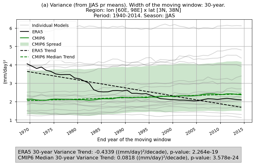
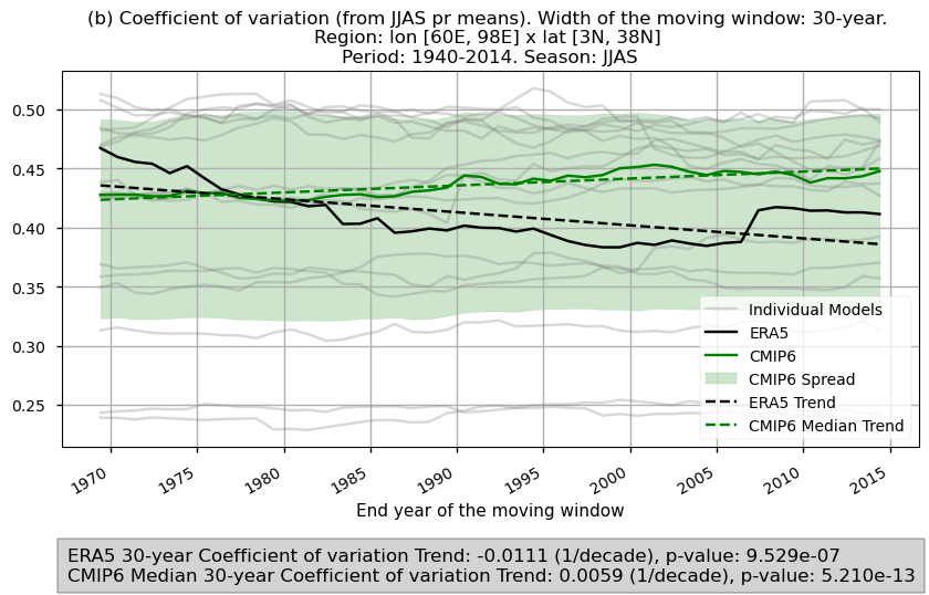
Fig 7. Time series of the spatially averaged values for the chosen variability formulations: (a) variance and (b) coefficient of variation for the JJAS mean precipitation over the period 1940–2014. The variance and coefficient of variation have been calculated using a 30-year window. Each time series displays the CMIP6 ensemble median (green), ERA5 (black), and individual models (grey), with dashed lines indicating the trend for the CMIP6 ensemble median and ERA5. The shaded area represents the ensemble spread. A grey box at the bottom displays the trend slope.

3.6. Results summary and discussion#

Substantial differences in spatial patterns can be observed depending on the formulation used to represent inter-annual variability during the Monsoon season (JJAS). This notebook uses two formulations: variance and the coefficient of variation (standard deviation divided by the mean).
Large differences in sign, magnitude, and spatial patterns of the biase are observed in the analyses using variance to represent inter-annual variability. Despite the differences across the subset of considered CMIP6 models, there is agreement in showing strong dependencies on orography and regions with high precipitation. These regions exhibit high biases due to elevated mean JJAS precipitation, although these biases are not necessarily large relative to the mean. Using the coefficient of variation eliminates this effect and may be more useful for assessing variability normalised to the mean amount of precipitation during the Monsoon period.
Generally, there are smaller differences depending on the model selection for the coefficient of variation, compared to the differences observed for the variance formulation. Inland north-western regions show large negative biases. These regions have, on average, near-zero or very low seasonal averages. One hypothesis to explain this may be that unusually wet seasons are underestimated in comparison to ERA5.
The time series displaying the evolution of variance and coefficient of variation (using a 30-year window) show a decline for ERA5 in the considered region. Based on the calculated trend, an approximate 50% reduction is estimated when comparing the start and end of the period for the variance formulation. This decrease is smaller when considering the coefficient of variation (11%). The ensemble median trend for the subset of considered CMIP6 models shows an increase of around 7% for the variance and 6% for the coefficient of variation over the same period, which differs from the trends observed in ERA5. It is important to note that the region studied is extensive. The time series represent spatially averaged values, and their results should be interpreted with care, as focusing on sub-regions within the domain may yield significantly different outcomes. Additionally, CMIP6 models exhibit notable inter-model spread, and a larger ensemble could also influence the results.
The time series results suggest that year-to-year variability in monsoon precipitation has become less pronounced according to ERA5. This is evident not only from the variance magnitude, which can be influenced by the evolution of the mean (shown to decrease during this period [3]), but also from the coefficient of variation, which removes this dependency by normalising the standard deviation with the mean.
What do the results mean for users?
- Importance of the selection of the variability formulation. The coefficient of variation has less dependency on orography because it is normalised by the mean. Moreover, the differences across the considered subset of models in the spatial pattern of the bias for the coefficient of variation appear to be smaller than in the case of variance. However, special attention needs to be given when using the coefficient of variation for the inland north-western region (where the seasonal mean precipitation is usually very low or near zero).
- ERA5 has biases [5][6]. This assessment uses it because a longer period is available and allows a more robust analysis of the temporal evolution of the variability. However the user may consider using other reference climate products such as the GPCP. This could lead to different results.
- ERA5 shows a decrease in inter-annual variability over the historical period for the considered region, while the CMIP6 ensemble median indicates a slight increase. It is important to consider a larger ensemble and note that the time series in this assessment represent spatially averaged values, which may yield different results when focusing on other sub-regions.
- Given the challenges in replicating the spatial patterns for variance and the coefficient of variation, as well as the difficulties in representing its temporal evolution, bias correction of CMIP6 projections may be essential for effectively using future projections of inter-annual precipitation variability. This enhancement could encourage the water management sector to adopt CMIP6 future projections, which can be extremely useful when designing strategies to adapt to projected changes in precipitation.
- Assessments using regional climate models (RCMs) may produce different results (not necessarily better) due to their higher spatial resolution, better representation of local processes, and more detailed treatment of orography and land-atmosphere interactions.

RESULTS NOTE:
It is important to note that the results presented are specific to the 16 models chosen, and users should aim to assess as wide a range of models as possible before making a sub-selection.

ℹ️ If you want to know more#

Key resources#

Some key resources and further reading were linked throughout this assessment.

The CDS catalogue entries for the data used were:

CMIP6 climate projections (Monthly - Precipitation): https://cds.climate.copernicus.eu/datasets/projections-cmip6?tab=overview
ERA5 monthly averaged data on single levels from 1940 to present (mean total precipitation rate): https://cds.climate.copernicus.eu/datasets/reanalysis-era5-single-levels-monthly-means?tab=overview

Code libraries used:

C3S EQC custom functions, c3s_eqc_automatic_quality_control, prepared by BOpen

References#

[1] Thornton, P. K., Ericksen, P. J., Herrero, M., and Challinor, A. J., 2014. Climate variability and vulnerability to climate change: A review. Global Change Biol. 20, https://doi.org/10.1111/gcb.12581

[2] Masroor, M., Rehman, S., Avtar, R., Sahana, M., Ahmed, R., Sajjad, H., 2020. Exploring climate variability and its impact on drought occurrence: evidence from Godavari Middle sub-basin, India. Weather and Climate Extremes. 30, 100277. https://doi.org/10.1016/j.wace.2020.100277

[3] Kulkarni, A. et al., 2020. Precipitation Changes in India. In: Krishnan, R., Sanjay, J., Gnanaseelan, C., Mujumdar, M., Kulkarni, A., Chakraborty, S. (eds) Assessment of Climate Change over the Indian Region. Springer, Singapore. https://doi.org/10.1007/978-981-15-4327-2_3

[4] Longobardi, A., Boulariah, O., 2022. Long-term regional changes in inter-annual precipitation variability in the Campania Region, Southern Italy. Theor Appl Climatol 148, 869–879. https://doi.org/10.1007/s00704-022-03972-2

[5] Ramon, J., Lledó L., Torralba, V., Soret, A., Doblas-Reyes, F.J., 2019. What global reanalysis best represents near-surface winds?. Q J R Meteorol Soc. 2019; 145: 3236–3251. https://doi.org/10.1002/qj.3616

[6] Hassler, B., and Lauer, A., 2021. Comparison of Reanalysis and Observational Precipitation Datasets Including ERA5 and WFDE5. Atmosphere, 12, 1462. https://doi.org/10.3390/atmos12111462

Testing the capability of CMIP6 GCMs to represent precipitation variability

Contents

5.1.9. Testing the capability of CMIP6 GCMs to represent precipitation variability#

🌍 Use case: Assessing the potential impacts of climate change on precipitation inter-annual variability over India for water management#

❓ Quality assessment question#

📢 Quality assessment statement#

📋 Methodology#

📈 Analysis and results#

1. Parameters, requests and functions definition#

1.1. Import packages#

1.2. Define Parameters#

1.3. Define models#

1.4. Define ERA5 request#

1.5. Define model requests#

1.6. Functions to cache#

2. Downloading and processing#

2.1. Download and transform ERA5#

2.2. Download and transform models#

2.3. Change some attributes#

3. Plot and describe results#

3.1. Define plotting functions#

3.2. Plot ensemble maps#

3.3. Plot model maps#

3.4. Plot bias maps#

3.5. Timeseries of the coefficient of variation#

3.6. Results summary and discussion#

ℹ️ If you want to know more#

Key resources#

References#