

5.1.7. Projections of future ice-free periods for the Arctic and Antarctic#
Production date: 2025-04-23
Produced by: Timothy Williams, Nansen Environmental and Remote Sensing Center (NERSC)
🌍 Use case: Scientific assessment of projected future ice-free conditions to inform product creation#
❓ Quality assessment question#
How likely are sea-ice-free conditions in the Arctic and Antarctic, and along the Arctic shipping routes, and when under which warming scenarios would they become more likely?
📢 Quality assessment statement#
These are the key outcomes of this assessment
Depending on the warming scenario, the Arctic itself has varying chances of being ice-free in the summer. While some authors project the first ice-free year as being before 2050 (regardless of warming scenario) (eg. SIMIP community, 2020; X. Zhao et al., 2022), we find (considering the full set of models proving sea ice concentration) more dependence on the warming scenario, with only 40% of models projecting an ice-free Arctic in 2050 under
ssp1_2_6while 60% of them project it underssp5_8_5. In 2070 this range has increased to between 50% and 85%. The period with high probabilities also lengthens according to the warming scenario, from just September inssp1_2_6to the 6-month period from June to December inssp5_8_5.The maximum Arctic area is projected to drop by between \(4\times 10^6\) km\(^2\) and \(8\times 10^6\) km\(^2\) from the pre-1960 levels of about \(17\times 10^6\) km\(^2\).
Around Antarctica, the climate models predict too little ice by quite a large margin, as seen by Roach et al. (2023) and the CDS assessment of historical sea ice extent, and this limits the conclusions that can be made about accessibility in this region. However with a definition of ice-free conditions consistent with the Arctic, we also see a similar pattern of increased overall probability and length of the period of high probabilities with increased warming.
We also see this behaviour for the two Arctic shipping routes, the Northern Sea Route (NSR) and the Transpolar Sea Route (TSR). There is higher probability of the TSR being ice-free in December than for the NSR. This is consistent with the results of other authors (Chen et al, 2023; Min et al., 2022).
📋 Methodology#
Related to this assessment are the assessments of sea ice extent and Arctic sea ice thickness in the CMIP6 historical experiment. The sea ice thickness bias is not directly relevant to this one, but it could have been used in subsetting the models.
For each experiment, we take all the models that provide sea ice concentration (SIC) outputs for our ensemble - i.e. we don’t do any subsetting of models in the results shown. We did do some sensitivity testing for the accessibility results however, and found no change to these results when using different model subsets. Specifically, noting that Pan et al. (2023) found that climate models whose ocean model component was NEMO (Nucleus for European Modelling of the Ocean) had noticeably reduced Arctic sea ice in projections compared to other climate models, we tried either excluding or only using such models. Users should still bear in mind that using a different subset could still effect results. For example, the SIMIP community (2020) selected models whose ensemble spread of sea ice area in the historical experiment included the satellite estimate. Alternatively, subsetting with “emergent constraints” (physically explainable empirical relationships) has been used to reduce the uncertainty in predictions. In examples of this approach, X. Zhao et al. (2022) used the accuracy of the mean April SIT and the response of the minimum sea ice area to the mean April SIT (compared to the value from Pan-Arctic Ice-Ocean Assimlation System, or PIOMAS) to select models, while Wang et al. (2021) used the accuracy of the surface air temperature and the sensitivity of the ice area to the surface air temperature. Another approach is to use weighted statistics (as done by J. Zhou et al., 2022), where weights are determined by model skill and interdependance.
We also do not consider the individual ensemble members available for each model, as the SIMIP community (2020) did, but only the ensemble mean for each model. This is done to save computational cost, but also avoids biasing the mean towards models with larger ensembles. Also note that we only use the monthly mean - considering daily means as done by Heuze & Jahn (2024) can lead to projected estimates of a much earlier first ice-free year (before 2030) than estimated using monthly means.
As well as the historical experiment, which has 33 models that output SIC, we use the following projection experiments, chosen because they provide a sufficiently large ensemble:
ssp1_2_6(22 models outputting SIC)ssp2_4_5(22 models outputting SIC)ssp3_7_0(21 models outputting SIC)ssp5_8_5(21 models outputting SIC)
The experiments are ordered by expected warming with ssp_1_2_6 giving the least warming (reaching 2.6 W/m\(^2\) in 2100, which is a kind of “best case” warming scenario) and ssp5_8_5 giving high warming (8.5 W/m\(^2\) in 2100).
The first number refers to which of the five Shared Socioeconomic Pathways (SSP) that the experiment corresponds to.
We calculate the minimum and maximum sea ice areas for the Arctic and Antarctica, show the historical and projected results as well as results derived from satellite observations, and show some climatological maps to show projected changes in the spatial distribution of SIC. To calculate the area we remap the model SIC onto the equal-area grids used by the observations. The ice-covered area in each grid cell can be determined from the SIC and the grid cell area, and then summed up to get the total ice-covered area. For each experiment, we then have an ensemble of areal time series (one from each model) and we plot the median and IQL (inter-quartile limits) of this ensemble. For the climatological maps we follow a similar procedure but average over time instead of space before plotting on the same grids that the observations use.
We also calculate the probability of them being “sea-ice-free” in the future as the fraction of models predicting the sea ice area dropping below a given region-dependent threshold (discussed below). We also do the same calculations for two Arctic shipping routes - the Transpolar Sea Route (TSR) and the Northern |Sea Route (NSR).
One point to note here is that we need to choose an area threshold for when a region is ice-free. A consequence of this is that the probabilities we calculate are a little arbitrary and so we should pay more attention to how they are changing with time than the absolute values. The thresholds we use to decide when the regions are ice-free are as follows. The ice-free threshold for the Arctic is usually taken as \(10^6\) km\(^2\) (e.g. Jahn et al., 2016). For the Antarctic this is too high since nearly all of the CMIP6 models significantly underestimate the Antarctic area and accordingly the minimum area for these models is less than \(10^6\) km\(^2\) even in the historical period (Roach et al., 2023; CDS assessment of historical sea ice extent). Therefore we choose the threshold to be \(0.25 \times 10^6\) km\(^2\), which is about one seventh of the pre-1970 Antarctic minima (according to the models) of about \(1.8 \times 10^6\) km\(^2\). This relationship is the approximate relationship in the Arctic, since the pre-1970 Arctic minima are about \(7 \times 10^6\) km\(^2\). For the two shipping routes, we also divide the pre-1970 Antarctic minima (again according to the models) by seven, giving thresholds of \(0.14 \times 10^6\) km\(^2\) for the NSR and \(0.21 \times 10^6\) km\(^2\) for the TSR.
Other authors have also studied accessibility of these and other shipping routes (eg. Chen et al, 2023;X. Zhao et al., 2022; Wang et al, 2021; Min et al., 2022; Li et al., 2021). For these authors, accessibility is determined by the polar class of the ship (how much ice strengthening the ship has) (if any) and the sea ice concentration and thickness. These variables are generally used as inputs into numerical ship-routing software like the Arctic Transport Accessibility Model (Smith & Stephenson, 2013) to create an ensemble of routes (created by using different start and end points for the journey) which are then analysed. Our approach, which would be applicable to open water vessels without ice strengthening, is comparatively simpler but is enough to give an overview of how likely the routes are to be clear and the effect of increased warming.
The “Analysis and results” section is organised as follows:
1. Import libraries, set parameters and definitions of functions
2. Download and transform data
3.1 Arctic sea ice minima and the projected probabilities of an ice-free Arctic
3.3 Antarctic sea ice minima and the projected probabilities of being ice-free around Antarctica
📈 Analysis and results#
1. Import libraries, set parameters and definitions of functions#
1.1 Import libraries#
Import the required libraries, including the EQC toolbox.
1.2 Set parameters#
Set the time period to be analysed with
year_startandyear_stop.Set the regions to be analysed with the list
sea_masks.Set the area thresholds for determining when each region is ice-free with
area_thresholds.Set the concentration threshold
sic_thresholdfor determining sea ice extent (we use 30% to be consistent with the ice edge product).Set the months we want to determine climatologies for with
clim_months.Set the averaging window (in years) for the climatologies for with
clim_length.Set the starting years for the climatologies for with
clim_start_years.Set the map projections for plotting climatologies with
projections.Set the map extents for plotting climatologies with
map_slices.Set the experiments to be considered with the list
experiments.Set the models to be evaluated with the dictionary
models_dict.
1.3 Define requests for CDS data#
Define the download requests in the format needed by the EQC toolbox.
1.4 Define functions to compute time series of extent and area#
apply_sea_maskchooses the region to analyse.compute_extent_and_area_from_siccomputes the extent and area from a sea ice concentration field.interpolate_to_satellite_gridinterpolates the model sea ice concentration to the reference grid (chosen to be the grid of the satellite sea ice concentration dataset).compute_interpolated_sea_ice_extent_and_areacallsinterpolate_to_satellite_gridto interpolate the model sea ice concentration to the reference grid and then callscompute_extent_and_area_from_sicto calculate the extent and area.
1.5 Functions to post-process and plot time series#
postprocess_datasetmakes the combined dataset easier to work with by making sure all each individual dataset uses the same calendar, and by renaming some variables and attributes.full_year_only_resampleresamples a time series to yearly, by either taking the minimum or maximum for the year.plot_timeseriesloops over each experiment and plots the median and the interquartile range (IQR) of the sea ice area of the ensemble of models. It also plots the area given by the satellite sea ice concentration products. The time series are reduced to yearly frequency according to the argumentreductionwhich is a string eg"min"or"max".plot_time_series_regional_reductionloops over two different time periods, the full CMIP6 period and a “zoomed-in” period (1980-2080 or 2020-2100), and callsplot_time_seriesfor each.
1.6 Functions to create the monthly climatologies#
compute_monthly_climatologyis the function that is used bydownload.download_and_transform. It takes in anxarray.Datasetand takes the temporal mean for each month, before callinginterpolate_to_satellite_gridto interpolate the result to the satellite grid.postprocess_climatologymakes the dataset easier to use by renaming some variables and ensuring the sea ice concentration has units%.get_monthly_climatology_modelfinalises the request to be passed todownload.download_and_transform, callsdownload.download_and_transform, and then callspostprocess_climatologyand returns the post-processed dataset.get_monthly_climatologies_cmip6creates the ensemble mean of monthly climatologies of the sea ice concentration, for a given experiment and time period. It does this by looping over the models in a given experiment and and callingget_monthly_climatology_modelfor each.
1.7 Functions to plot climatology maps#
get_datasets_eumetsat_climdownloads satellite data for each hemisphere for one day. These datasets will be used to add a mask to CMIP6 projection data to improve their visual appearance.make_sic_mapsplots the climatology maps for each experiment (in columns) and time period (in rows).compare_sic_mapsis a wrapper that organises the inputs tomake_sic_mapsbefore calling it.
1.8 Functions to plot the access to a given area#
plot_sea_masksmakes maps illustrating where we define the transpolar shipping route and the northern sea shipping route.get_access_tablesorts the time series of sea ice area to make a dataset with dimensionsyearandmonthcontaining the probability that a region will be clear for that year and month. The probability is calculated by considering each model in an experiment.get_access_tablesloops over each CMIP6 projection experiment and callsget_access_table.plot_access_tablesthen plots the probability of a region being clear for each experiment by year and month.plot_access_vs_month_one_yearplotsProbability clearagainstmonthfor all the experiments and for a given year. That is, it combines vertical slices of the access tables for all the different experiments.plot_access_vs_monthloops over a number of years and callsplot_access_vs_month_one_year.
2. Download and transform data#
2.1 Set some downloading parameters#
io_kwargsare some options to speed-up the downloading.common_kwargsadds thetransform_funcoption to makedownload.download_and_transformtransform the data usingcompute_interpolated_sea_ice_extent_and_area.transform_func_kwargsare options to be passed tocompute_interpolated_sea_ice_extent_and_area.interpolation_kwargsare options for interpolation.region_name_mappermakes the region names more user friendly.
2.2 Download and transform satellite data for time series#
Loops over the two satellites and the four masks to get time series of sea ice extent and area for the satellite sea ice concentration products. download.download_and_transform downloads the data and transforms it with compute_interpolated_sea_ice_extent_and_area before saving it to disk. The dataset is then post-processed with postprocess_dataset. The time series are stored in the dictionary datasets_satellite.
2.3 Download and transform CMIP6 data for time series#
Loops over each model in each experiment, and the four masks, to get time series of sea ice extent and area for the CMIP6 models. For each combination, download.download_and_transform downloads the data and transforms it with compute_interpolated_sea_ice_extent_and_area before saving it to disk. The dataset is then post-processed with postprocess_dataset. The time series are stored in the dictionary datasets_cmip6.
2.4 Download and process climatologies for CMIP6 projections#
This step loops over each hemisphere, each model in each experiment, and each time period, and calls get_monthly_climatologies_cmip6 to get the ensemble mean (average over all models in an experiment) for each hemisphere, experiment and time period. The climatologies are stored in the dictionary datasets_cmip6_clim.
3. Results#
In this section we plot yearly minima and maxima for sea ice area, for the Arctic and Antarctic. We also estimate the probability that a region is ice-free, by taking the ensemble of models and using the percentage of models predicting it as having low enough area as the probability. We chart this by month-by-month to also see how much of the year periods with a high chance of being ice-free are happening.
3.1 Arctic sea ice minima and the projected probabilities of an ice-free Arctic#
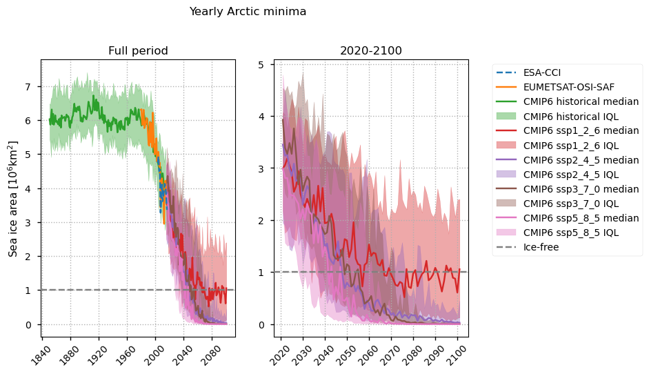
In the Arctic region, the yearly minimum in sea ice area shows a clear effect of increased warming. Before about 1990 the historical CMIP6 is relatively constant. After this time however it drops rapidly. This agrees quite well with the satellite data when they are available. As we come to the start of the projection period (2015-2100), the yearly minima continues to drop. The minimum area is highest for the ssp1_2_6 experiment and its median plateaus around the ice-free level, so about half the models predict the Arctic will be ice-free in the projection period under this scenario. The medians for the ssp2_4_5 and ssp3_7_0 minimum extents are similar, both reaching the ice-free level about 2050, and even dropping close to zero by the end of the century. The ssp5_8_5 median is consistently the lowest and reaches the ice-free level around 2040. The median drops to near zero around 2070.
The yearly minimum in sea ice area follows mostly the same pattern, although the time when the median and lower quartile reach zero is slightly later since there is no concentration threshold used in the calculation (a grid cell is classed as ice-free if the concentration is below 30%).
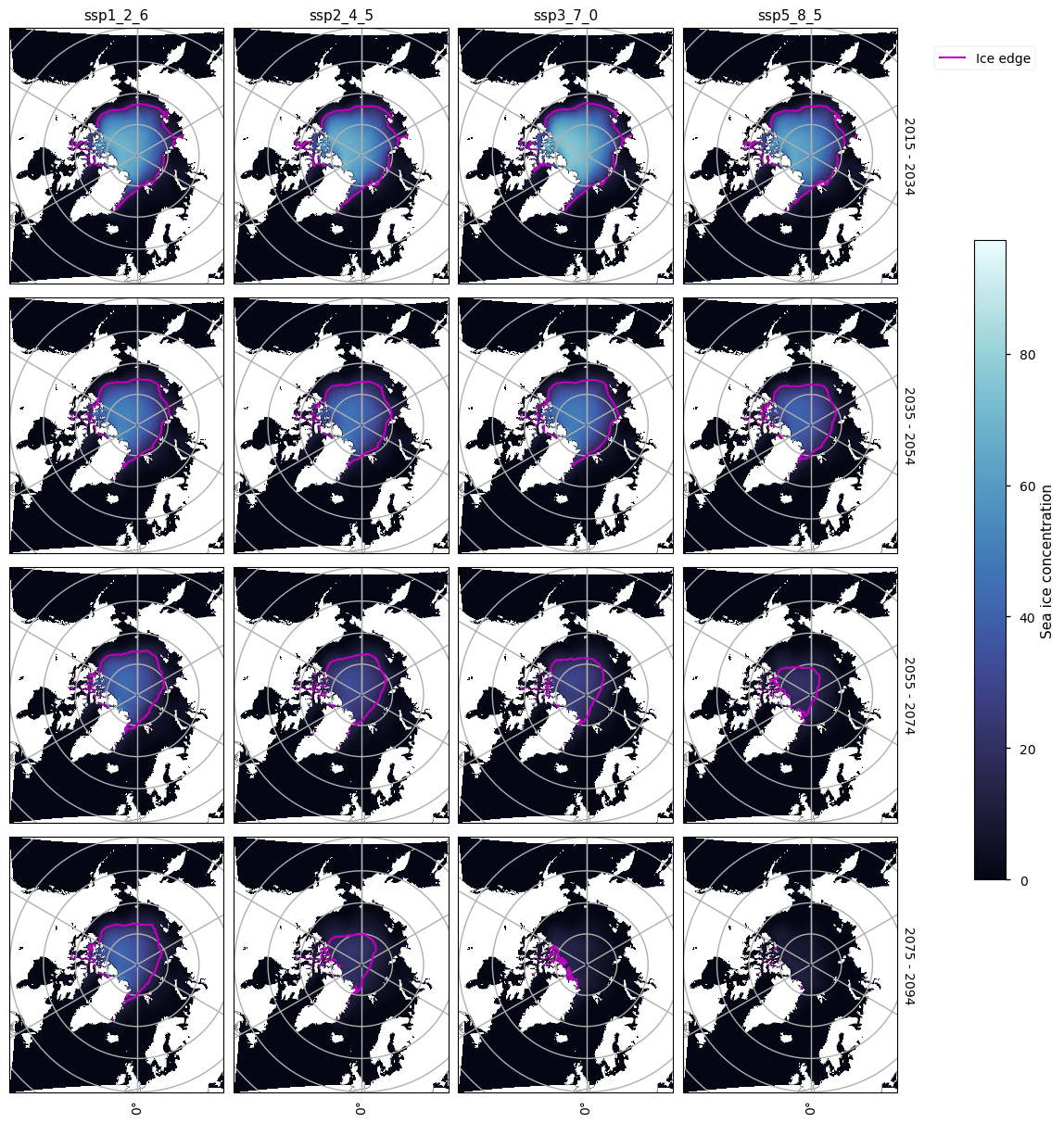
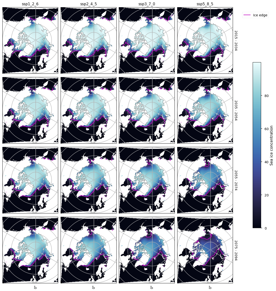
The maps below show the spatial pattern of the decrease in sea ice cover by plotting the ensemble mean of the sea ice concentration for a series of 20-year climatologies for the month of September. The magenta lines plot the ice edge (15% concentration contour). Going from left to right (increasing the amount of warming in the projection), there is quite a big difference, especially from 2035. From 2055 only the ssp_1_2_6 experiment has a significant amount of ice.
The heat maps below show the proportion of models having a minimum Arctic sea ice area less than \(10^6\) km\(^2\). For the ssp1_2_6 experiment, the chances of being ice-free in September reach 20% around 2040, 40% around 2050 and 50% around 2070. In August there are consistently 40-50% probabilities after 2080, while in October the chances are about 20-30% from this time. From 2090, about 15% of the models predict ice-free conditions in July under this warming scenario.
We can see however that the chances are being overestimated (perhaps indicating a bias of about 10%) since some years in the past (at time of writing i.e. 2015-2024) have 10% chance of the Arctic being ice-free (1 in 10 models predict this) while it has never been observed yet. Choosing a different subset of models could also avoid this bias.
In the ssp2_4_5 experiment, the pattern is similar but the probabilities have increased somewhat. In September they are above 80% from about 2085, with it being 95-100% for three of the later years. In August and October the chances reach about 70% (in 2085 and 2093 respectively), and 20% of the models are predicting ice-free conditions in July and November.
In the ssp3_7_0 experiment, there are now 85%-90% chances of being ice-free in August-October after about 2085. The chances in July and November have also increased (above 40% after about 2083, and sometimes reaching 60%), and there is also a 20%-30% chance of it being ice-free in June and December from about 2095.
In the ssp5_8_5 experiment, there are now chances of the Arctic being ice-free from August to October of around 70-80% from about 2070. In September, the chances of being ice-free are consistently over 80% from around 2065. July and November have high chances (70%-85%) of an ice-free Arctic in the last decade or two under this scenario, and the chances of June and December start to become significant earlier than under ssp3_7_0. In this experiment (ssp5_8_5), even May and January have 20% probability in the last 5 years or so.
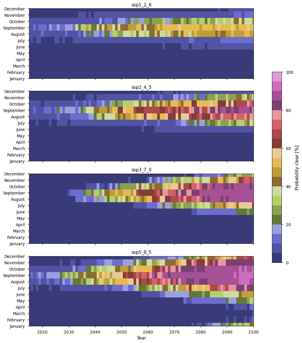
In summary, the heat maps above show that as the warming increases, we can clearly see that the overall probability of being ice-free is increasing, and the length of the season where there is high probability is also increasing from just September (ssp1_2_6) to the 6-month period from June to December (ssp5_8_5).
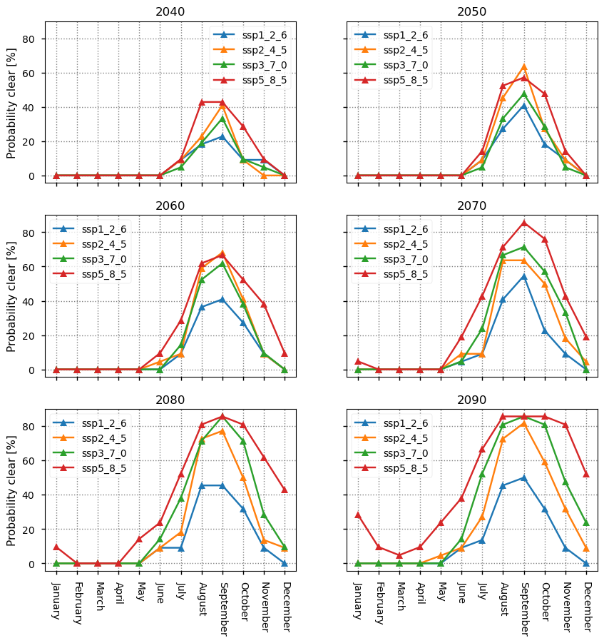
This can also be seen in the plots below, where we compare the experiments more directly by plotting the monthly probabilities for a selection of years.
In the years before 2060, the probabilities are not ordered by warming strength, but around 2060 ssp3_7_0 reaches the ssp2_4_5 level, and after that year the probabilities’ order does correspond to warming strength.
In 2040, the maximum probability ranges from about 20% to 40%; in 2050 and 2060 it ranges from about 40% to 60%; in 2070, 2080 and 2090 it ranges from about 45% to about 85%. In the latter three years the main effect is the widening of the season with the highest probabilities.
Comparing to other authors estimates, the SIMIP community (2020) found that nearly all of their selected models projected ice-free conditions by 2050, regardless of warming scenario. X. Zhao et al. (2022) agree with this - they projected the first ice-free year to be \(2049\pm 12\) under ssp2_4_5 and \(2043\pm 9\) under ssp5_8_5, giving a similar range to the SIMIP community (2020). While our 2050 probability of just under 60% for ssp5_8_5 is quite high, 40% for ssp1_2_6 is quite a lot lower. This difference possibly reflects the effect both of using a different subset of models and of using the full ensemble set provided for each model, as SIMIP community (2020) did (instead of just using the ensemble mean for each model).
3.2 Arctic sea ice maxima#
Like the Arctic minimum in sea ice area, the maximum sea ice area is constant until about 1990 the historical CMIP6 is relatively constant, before starting to drop rapidly. However, unlike with the minimum area, there is a clear bias in this variable, with both the ERA5 reanalysis and the CMIP6 ensembles overestimating it by about \(1.5\times10^6\)km\(^2\). As we come to the start of the projection period (2015-2100), the yearly maxima continues to drop. Unlike with the minima, the maximum sea ice area shows a clear response to increased warming - as the warming increases the median Arctic maximum area drops. The experiment with the most warming (ssp5_8_5) also shows a very large spread in this variable by 2100.
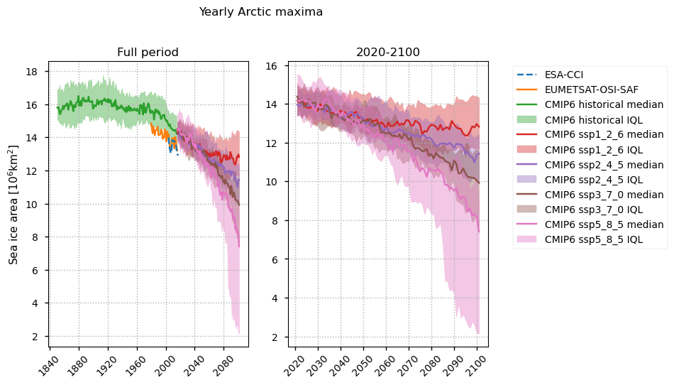
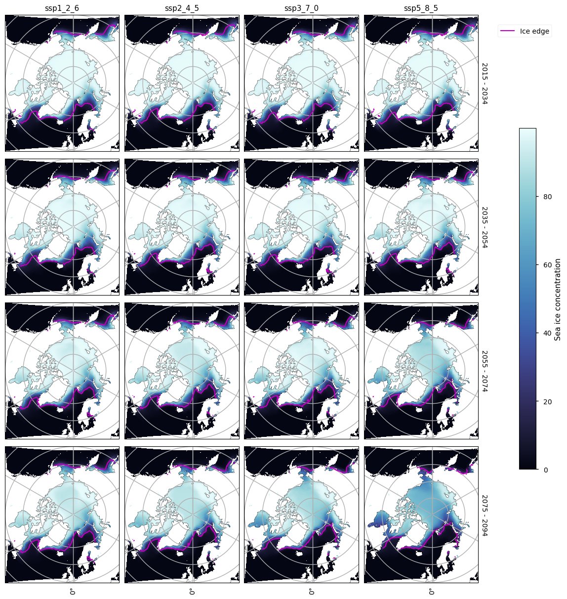
Looking at the maps below, we can see that there is not too much difference between the maps in March before about 2055. After this however, the ssp5_8_5 experiment especially starts to have reduced concentration in the central Arctic, and also in the Hudson Bay. The ssp3_7_0 experiment also shows this pattern to some extent. The drop in maximum sea ice area with time can also be seen, e.g. in the Bering and Labrador Seas.
3.3 Antarctic sea ice minima and the projected probabilities of being ice-free around Antarctica#
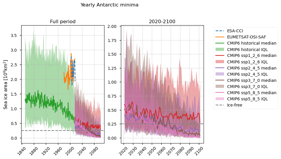
The CMIP6 models show a large bias in the Antarctic minimum sea ice area compared to the satellite data, underestimating it by about 1-\(2\times10^6\)km\(^2\). The satellites seem to show a relatively constant minimum, while there is a steady drop predicted by the CMIP6 models in this time period when observations are available (1979-2017).
Keeping in mind the large bias in the CMIP6 models in this area (Roach et al., 2023; CDS assessment of historical sea ice extent), the modelled Antarctic minimum in sea ice area shows a clear effect of increased warming. After about 1960 the CMIP6 ensemble median starts to slowly drop, and then after 2015 the rate depends on the warming scenario. The median only reaches our ice-free limit of \(0.25\times10^6\) km\(^2\) under the ssp3_7_0 and ssp5_8_5 scenarios, but the ssp2_4_5 median is close to it. Under the ssp1_2_6 scenario the area stays about \(0.4\times 10^6\) km\(^2\) from about 2040. The spread of the models is quite high.
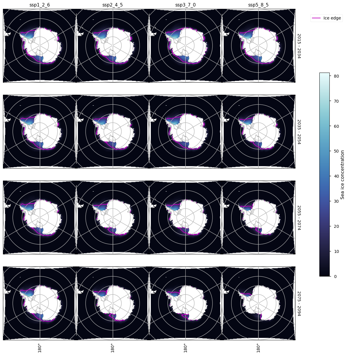
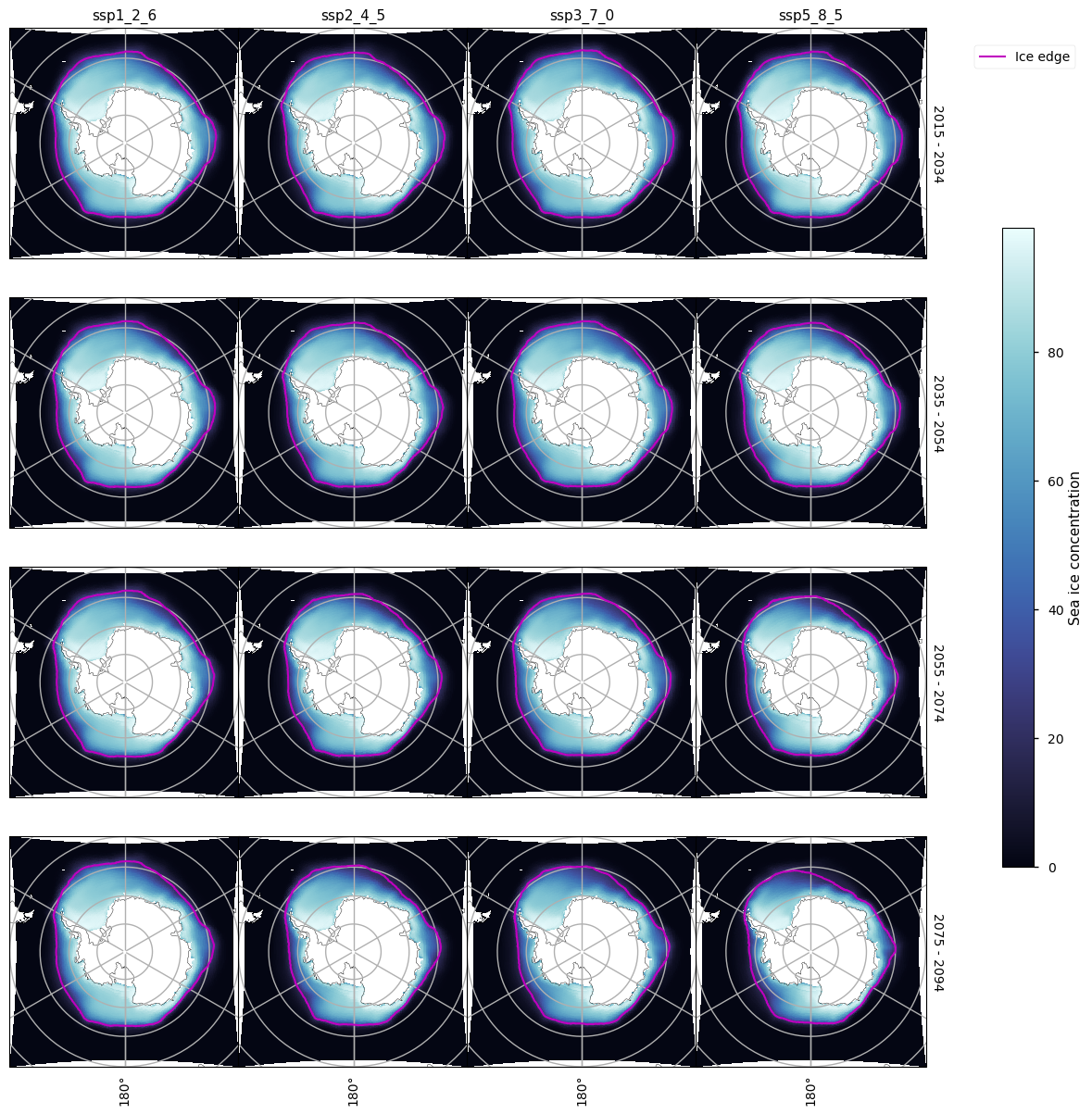
A clear effect of climate change can be see in the maps below of the Antarctic sea ice concentration for March. Apart from the ssp1_2_6 experiment, there is very little ice outside the Weddell and Ross Sea, and the ssp5_8_5 has mostly lost its ice in the Ross Sea by 2075.
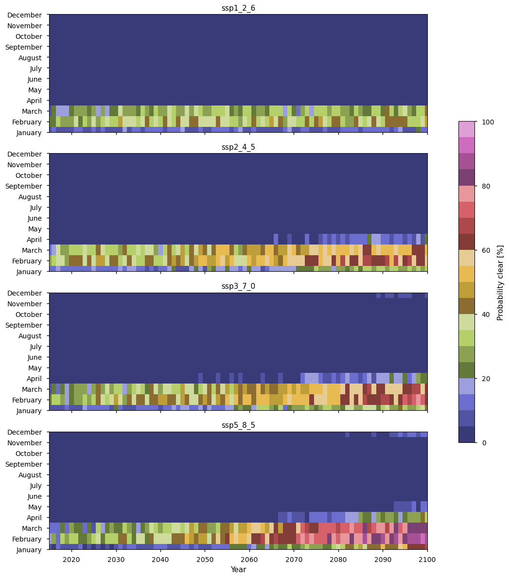
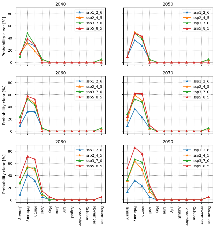
The heat maps below show the proportion of models dropping below \(0.25\times10^6\) km\(^2\) for a given month and year, and below them we compare the monthly probabilities more directly for all the experiments for a selection of years.
As with the Arctic, increased warming increases the overall probability and also the length of the period when there is high probability. However, unlike the Arctic, the Antarctic region has lower chance of being ice-free, only getting consistently over 70% only in the warmest scenario ssp5_8_5. The chances in February reach 50% around 2040 and 80% around 2088 in that experiment.
In March and January the probability also reaches 60% (in 2070 and 2095 respectively), and even 70% (from about 2080 in March).
The ssp_2_4_5 and ssp_3_7_0 experiments show similar probabilities, consistently reaching 60% in February in the last two decades or so. In March they get to 50% from about 2080 (a few years earlier under ssp_2_4_5).
The ssp1_2_6 experiment has probabilities of being ice-free oscillating between 20%-40% in February, and between 20%-35% in March.
3.4 Antarctic sea ice maxima#
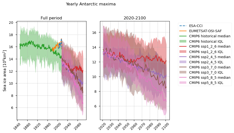
The projected Antarctic sea ice maxima behave in a similar way to the Arctic maxima with time and warming, with a similar relative drop (30%-50%). The CMIP6 models again show a large bias in the Antarctic sea ice area compared to the satellite data, although the difference is less at the start of the start of the satellite period (1979). However, since the satellites show a slight increase in minimum area, while there is a steady drop predicted by the CMIP6 models, the difference increases with time, reaching about \(2\times10^6\)km\(^2\) by 2015.
Less effect can be seen in the maps below of the ensemble mean Antarctic sea ice concentration in September than in March. For the ssp1_2_6 experiment, there is little difference between the last time period and the first, but there small decreases in area, which are relatively even around the continent, visible for the other experiments. In the last two time periods, there is also a slight decrease in area as the warming increases.
3.5 Projected access to Arctic shipping routes#
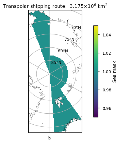
We consider two Arctic shipping routes, the Transpolar Shipping Route (TSR) and the Northern Sea Route (NSR). We do not consider the Northwest Passage (NWP) since the climate models generally don’t have enough resolution to represent the Canadian archipelago. The figure below shows our definition of these two routes.
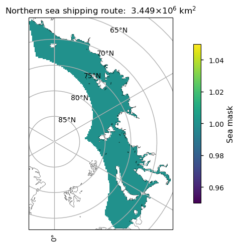
3.5.1 Northern sea route#
In the plots below we can see the minimum sea ice area in the NSR as stable at about \(10^6 \)km\(^2\) until about 1970 when it starts dropping. The historical area is fairly close to the observations in this area, athough they are initially a bit low and a bit high after about 2005. Most experiments’ median have dropped below the ice free level by 2040.
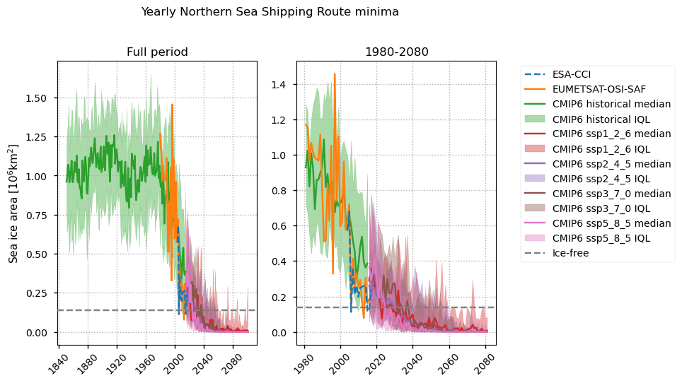
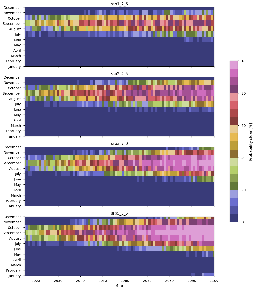
The heat maps below show the proportion of models dropping below \(0.14\times10^6\) km\(^2\) for a given month and year, and below them we compare the monthly probabilities more directly for all the experiments for a selection of years.
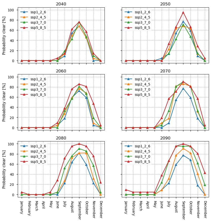
We can see even in the experiment with the least warming, there is a high chance of the Northern Sea Route (NSR) being clear in September, especially after about 2040, when the probability reaches about 70%. After this the probabilty fluctuates between about 70% and 80%. August has quite high probabilities too, getting to around 70% around 2060. The probability in October reaches about 50%, while it reaches about 20% in July. The chances increase as the experiments change to produce more warming, and the chances of having the NSR clear in November and July start to increase as well. In November and July ssp3_7_0 has about 60-70% (sometimes higher) chance after 2082 or 2083. ssp5_8_5 has 80% chance in November and 70-80% chance in July, both from about 2075. In July ssp3_7_0 has about 60-70% chance after 2080, while ssp5_8_5 has 80% chance from about 2075. The experiment ssp5_8_5 even has 40-50% chance of it being clear in December in later years, and 80-100% of the models are projecting the NSR to be free in August, September, and October from about 2055 under this scenario.
The probabilities shown below for September in 2040 and 2050 are only slightly lower than the results of Chen et al. (2023) (see Figures 6a and 6b), who estimated the probability (averaged over 2045-2055) of the Sannikov Strait being passable by open water vessels (without ice strengthening) of 60% under ssp1_2_6 and 100% under ssp5_8_5. The size of their navigability window (about July-November) is also similar to ours. This strait (along with the Dmitry Laptev Strait which had slightly lower passability than the Sannikov Strait) is key for the overall passability of the NSR overall. This consistency is reassuring given the quite different methods of calculating the probabilities and the different subsets of the climate models used.
3.5.2 Transpolar shipping route#
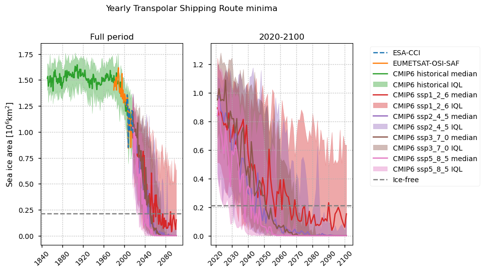
In the plots below we can see the minimum sea ice area in the TSR as stable at about \(1.5 \times 10^6 \)km\(^2\) until about 1970 when it starts dropping. The area from historical experiment is fairly close to the observations in this area. Most experiments’ median have dropped below the ice free level by 2050, with the exception of the ssp1_2_6 experiment, which is not consistently beneath it until about 2070. This experiment has quite a large spread compared to the others.
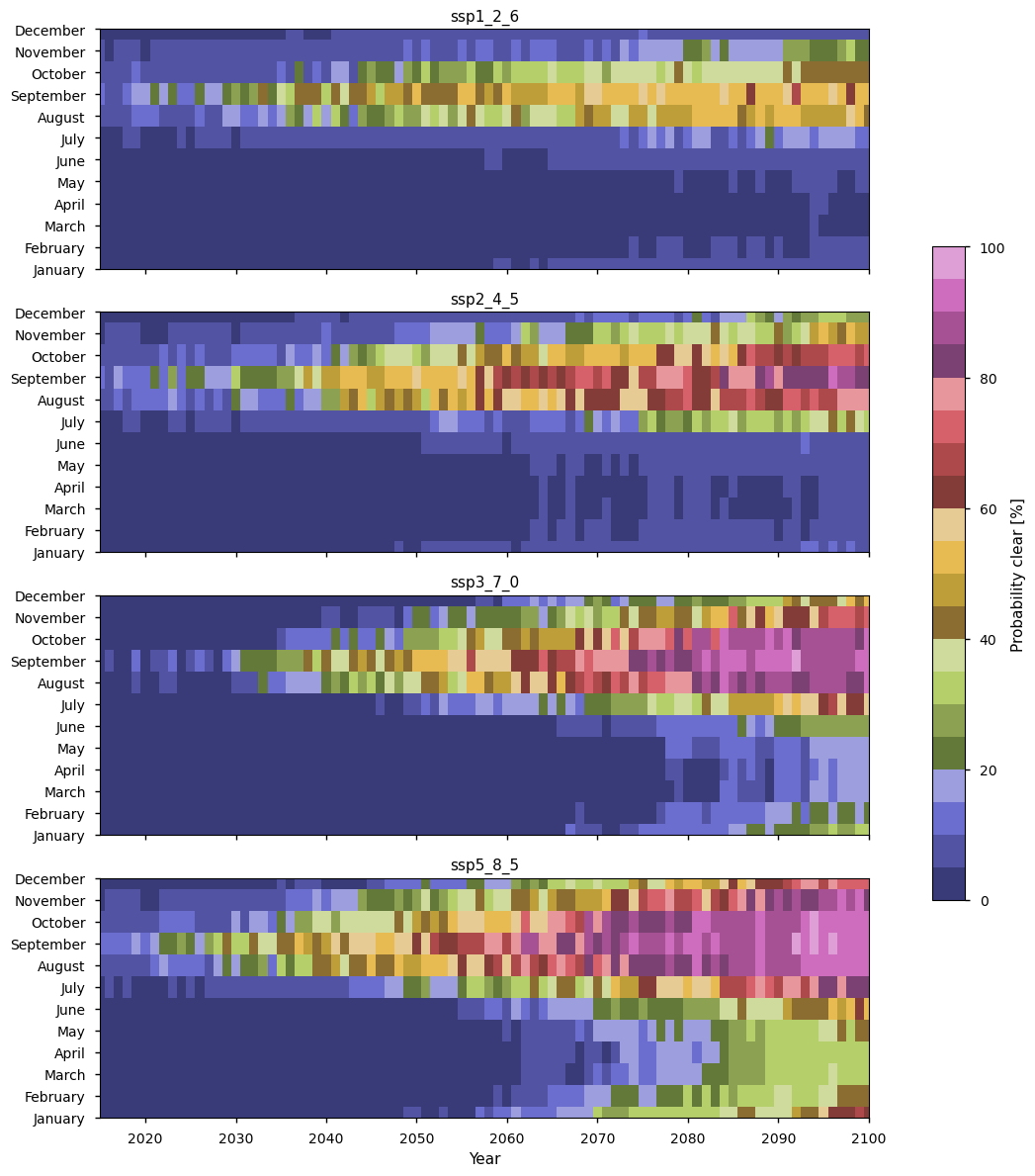
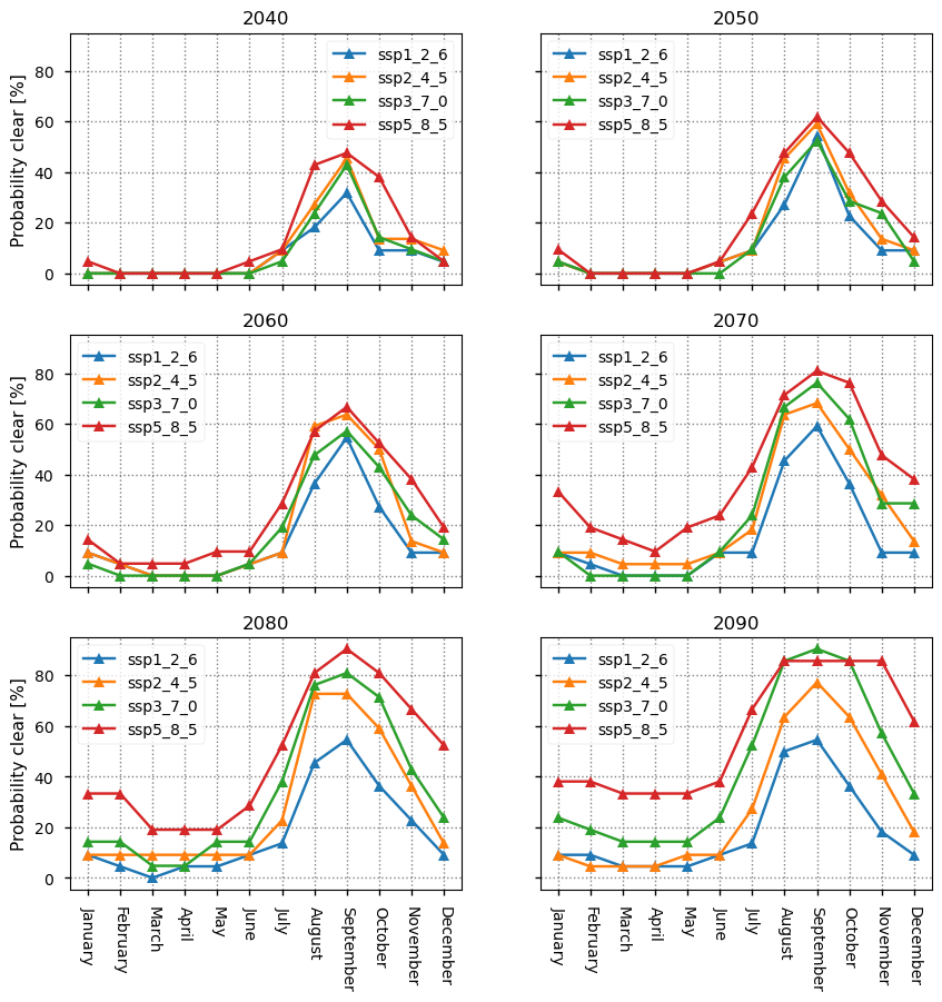
The heat maps below show the proportion of models dropping below \(0.21\times10^6\) km\(^2\) for a given month and year, and below them we compare the monthly probabilities more directly for all the experiments for a selection of years.
The Transpolar shipping route (TSR) has slightly lower chances of being ice-free in the months August-October than the NSR but somewhat surprisingly it is a bit higher in other months, with it having some chance of it being clear in winter months in the experiments with higher warming.
For example, under ssp5_8_5 there is a 35% chance of the TSR being clear from February to May after 2089 (after 2085 for February), and there is more than 60% chance of it being clear in December from about 2088, and the same chance in January from 2095.
Under ssp3_7_0 there is more than 20% chance of the TSR being ice-free in December, and also in January from 2090.
The maps below plot the ensemble mean sea ice concentration for December for a series of time intervals between 2015 and 2095. In the 2075-2095 period, the ssp5_8_5 has a distinct gap where we have defined our TSR, while there is still ice off the Russian coast blocking the NSR. The effect is also present to a lesser extent for the ssp2_4_5 and ssp3_7_0 xperiments, so perhaps ice-strengthened vessels could still traverse the TSR under these scenarios also. This is consistent with the results of Min et al (2022) (see Figure 3), who found that from 2080 to 2100, the TSR would be a more robust option than the NSR or the North-West Passage for open water vessels.
ℹ️ If you want to know more#
Key resources#
Introductory sea ice materials:
Introductory CMIP6 materials:
Code libraries used:
C3S EQC custom functions developed by B-Open
References#
Chen, J. L., Kang, S. C., Wu, A. D., Chen, L. H., & Li, Y. W. (2023). Accessibility in key areas of the Arctic in the 21st mid-century. Advances in Climate Change Research, 14(6), 896-903, https://doi.org/10.1016/j.accre.2023.11.011 .
Chen, J., Kang, S., You, Q., Zhang, Y., & Du, W. (2022). Projected changes in sea ice and the navigability of the Arctic Passages under global warming of 2℃ and 3℃. Anthropocene, 40, 100349, https://doi.org/10.1016/j.ancene.2022.100349 .
Chen, J. L., Kang, S. C., Guo, J. M., Xu, M., & Zhang, Z. M. (2021). Variation of sea ice and perspectives of the Northwest Passage in the Arctic Ocean. Advances in Climate Change Research, 12(4), 447-455, https://doi.org/10.1016/j.accre.2021.02.002 .
Davy, R., and S. Outten (2020). The Arctic Surface Climate in CMIP6: Status and Developments since CMIP5. J. Climate, 33, 8047–8068, https://doi.org/10.1175/JCLI-D-19-0990.1 .
Heuzé, C. & Jahn, A. (2024). The first ice-free day in the Arctic Ocean could occur before 2030. Nat. Commun. 15, 10101, https://doi.org/10.1038/s41467-024-54508-3 .
Jahn, A., Kay, J. E., Holland, M. M., & Hall, D. M. (2016). How predictable is the timing of a summer ice‐free Arctic? Geophysical Research Letters, 43(17), 9113-9120 , https://doi.org/10.1002/2016GL070067 .
Jahn, A., Holland, M.M. & Kay, J.E. (2024). Projections of an ice-free Arctic Ocean. Nat. Rev. Earth. Environ. 5, 164–176, https://doi.org/10.1038/s43017-023-00515-9 .
Li, X., Stephenson, S. R., Lynch, A. H., Goldstein, M. A., Bailey, D. A., & Veland, S. (2021). Arctic shipping guidance from the CMIP6 ensemble on operational and infrastructural timescales. Climatic Change, 167, 1-19, https://doi.org/10.1007/s10584-021-03172-3 .
Melia, N., Haines, K., and Hawkins, E. (2016). Sea ice decline and 21st century trans-Arctic shipping routes, Geophys. Res. Lett., 43, 9720–9728, https://doi.org/10.1002/2016GL069315 .
Min, C., Yang, Q., Chen, D., Yang, Y., Zhou, X., Shu, Q., & Liu, J. (2022). The emerging Arctic shipping corridors. Geophysical Research Letters, 49(10), e2022GL099157. https://doi.org/10.1029/2022GL099157 .
Pan, R., Shu, Q., Wang, Q., Wang, S., Song, Z., He, Y., & Qiao, F. (2023). Future Arctic climate change in CMIP6 strikingly intensified by NEMO‐family climate models. Geophysical Research Letters, 50(4), e2022GL102077, https://doi.org/10.1029/2022GL102077 .
Roach, L. A., J. Dörr, C. R. Holmes, F. Massonnet, E. W. Blockley, D. Notz, T. Rackow, M. N. Raphael, S. P. O’Farrell, D. A. Bailey, and C. M. Bitz (2020). Antarctic sea ice area in CMIP6. Geophysical Research Letters, 47, e2019GL086729, https://doi.org/10.1029/2019GL086729 .
SIMIP Community (2020). Arctic sea ice in CMIP6. Geophysical Research Letters, 47, e2019GL086749, https://doi.org/10.1029/2019GL086749 .
Smith, L. C., & Stephenson, S. R. (2013). New Trans-Arctic shipping routes navigable by midcentury. Proceedings of the National Academy of Sciences, 110(13), E1191-E1195, https://doi.org/10.1073/pnas.1214212110 .
Wei, T., Yan, Q., Qi, W., Ding, M., & Wang, C. (2020). Projections of Arctic sea ice conditions and shipping routes in the twenty-first century using CMIP6 forcing scenarios. Environmental Research Letters, 15(10), 104079, https://doi.org/10.1175/JCLI-D-19-0990.1 .
Wang, B., Zhou, X., Ding, Q., & Liu, J. (2021). Increasing confidence in projecting the Arctic ice-free year with emergent constraints. Environmental Research Letters, 16(9), 094016, https://doi.org/10.1088/1748-9326/ac0b17 .
Zhao, J., He, S., Wang, H., & Li, F. (2022). Constraining CMIP6 Projections of an ice‐free Arctic Using a weighting scheme. Earth’s Future, 10(10), e2022EF002708, https://doi.org/10.1029/2022EF002708 .
Zhou, X., Wang, B., & Huang, F. (2022). Evaluating sea ice thickness simulation is critical for projecting a summer ice-free Arctic Ocean. Environmental Research Letters, 17(11), 114033, https://doi.org/10.1088/1748-9326/ac9d4d .