

1.3.1. Glacier mass change data from satellite and in-situ observations: uncertainty analysis for glaciological and climate change monitoring#
Production date: 31-05-2025
Dataset version: WGMS-FOG-2023-09
Produced by: Yoni Verhaegen and Philippe Huybrechts (Vrije Universiteit Brussel)
❓ Quality assessment question#
“Is the glacier mass change dataset sufficiently adequate in terms of its uncertainty to effectively monitor and evaluate global (cumulative) glacier mass changes over time, including their associated impacts on global sea level rise?”
Glaciers significantly impact global sea-level rise, freshwater resources, natural hazards, hydro-power generation, recreation and tourism. Assessing glacier mass changes due to climate warming is therefore crucial for addressing these issues. The “Glacier mass change gridded data from 1976 to present derived from the Fluctuations of Glaciers Database” (version WGMS-FOG-2023-09) on the Climate Data Store (CDS), offers a global coverage of glacier mass changes by integrating in-situ, aerial, and satellite data [1, 2]. The gridded glaciers mass change dataset that is on the CDS is currently one of the most complete dataset of glacier mass change data in terms of its spatial coverage. It is generally considered the main reference dataset to determine long-term glacier mass changes across the globe.
When measured over a long period and at extended geographical scales, trends in glacier mass balance can be considered a clear indicator of global climate change [3]. Despite some known issues, this dataset provides valuable insights into glacier mass changes across spatial and temporal scales. In that regard, this notebook investigates how well the dataset can be used to quantify the link between glacier melt and glacier-related sea level contributions. More specifically, the notebook evaluates whether the dataset is of sufficient maturity and quality for that purpose in terms of its uncertainty (i.e. accuracy and precision).
📢 Quality assessment statements#
These are the key outcomes of this assessment
The C3S glacier mass change dataset is a mature and quality-rich dataset that allows users to capture the changing state of glaciers on a local, regional and global scale. The data come with a quantitative pixel-by-pixel error estimate in the form of precision errors (reported as 1.96 times the standard deviation), that generally decrease in magnitude over time. As a consequence, the most recent years (after 2000) meet proposed international standards of uncertainty thresholds proposed by GCOS. The uncertainty that comes with the data is, however, highly spatially and temporally variable, with areas like the peripheral glaciers in Greenland and Antarctica exhibiting higher glacier mass change errors. Hence, not all pixels meet the minimum uncertainty threshold proposed by GCOS, of which users should take note. However, when seen as a whole, the majority of the pixels meet the proposed thresholds for uncertainty.
The dataset is highly suitable to monitor and derive global (cumulative) mass changes over time and to, for example, assess the corresponding impact of their shrinkage. The dataset furthermore has sufficient quality in terms of its consistency with respect to spatial (i.e. global) and temporal (i.e. since 1975-76) coverage for climate change monitoring to become useful and to be able to draw reliable conclusions. Some potential key limitiations include the lack of detailed sampling information, the limited use for individual glacier-scale (smaller than the pixel-scale) applications, and the fact that not all mass changes considered in the dataset directly contribute to sea-level changes (which is nevertheless assumed to be the case). Due to variations in data collection methods and sources, data consistency along the data may furthermore be affected.
📋 Methodology#
Dataset description#
The mass balance of a glacier is the difference between mass gained (mainly from snow accumulation) and mass lost (by meltwater runoff or solid ice discharge into lakes/the ocean), which is the same as the net mass change of a glacier over its surface area \(A\):
\(\Delta{M} = \dfrac{1}{A} \int\limits_{A} b_a dA - \dfrac{1}{A} \int\limits_{P} d_a dP\)
where:
\(b_a = \int\limits^{t_1}_{t_0}b_s dt\), with \(b_s = ACC - ABL\) [kg m\(^{-2}\) yr\(^{-1}\)]
\(d_a = \int\limits^{t_1}_{t_0}d_g dt\), with \(d_g = \rho_{i} \cdot H \cdot \overline{V_P}\) [kg m\(^{-1}\) yr\(^{-1}\)]
The first term represents the the total annual surface mass balance (i.e. the difference between accumulation and ablation), whereas the second term encompasses the total annual ice discharge across the grounding line \(g\) with perimeter \(P\). Here, \(\rho_{i}\) is the ice density, \(H\) ice thickness and \(\overline{V_P}\) the gate-perpendicular vertically averaged horizontal velocity at the grounding line location. The latter term is considered zero for land-terminating glaciers. Other terms can be included as well, such as the basal and internal mass balances.
In general, the basis for the derived gridded mass changes are individual measurements (mainly glaciological in-situ local annual surface mass balance measurements) and geodetic air or spaceborne elevation change data (a surface elevation/ice thickness change or an ice volume change over time). These data are converted into an averaged specific mass balance value (i.e. mostly reported with units of meter water equivalent and often shortened to m w.e.) for an individual glacier. Afterwards, the data are submitted to the World Glacier Monitoring Service (WGMS). Further processing of the data results in a glacier mass change product reported over a 0.5° global grid dating back until the 1975-76 hydrological year. Each grid cell therefore contains a time series of total glacier mass change (in Gt yr⁻¹) or mass balance data (in m w.e. yr⁻¹) of all glaciers within the specific grid cell. In this notebook, we use version WGMS-FOG-2023-09. For a more detailed description of the data acquisition and processing methods, we refer to the documentation on the CDS and the ECMWF Confluence Wiki (Copernicus Knowledge Base).
It is important to note that the glaciers with an annual glaciological sample (ca. 500 glaciers) form the basis for the determination of annual mass changes from the remaining glaciers through a complex algorithm of spatial/temporal interpolation and (area-weighted) averaging of these mass change data [2]. Hence, not all glaciers in the dataset exhibit a time series of directly measured annual in-situ mass balance observations, but most glaciers in the dataset are either unobserved or only have (limited and mostly multi-annual) geodetic mass change data available. Glacier mass change data with these geodetic samples are also more prone to uncertainties in general, for example due to uncertainties related to volume to mass conversions.
Structure and (sub)sections#
1. Data preparation and processing
2. Glacier mass changes and their uncertainty estimates in space and time
3. Quantifying global (cumulative) glacier mass changes and their error estimates since 1975-1976
4. Quantification of glacier-related contributions to global sea level change
📈 Analysis and results#
1. Data preparation and processing#
1.1 Import packages#
First we load the packages:
1.2 Define request and download#
Then we define the parameters, i.e. for which years we want the glacier mass change data to be downloaded:
Then we define requests for download from the CDS and download and transform the glacier mass change data.
Downloading glacier mass change data...
100%|██████████| 1/1 [00:06<00:00, 6.66s/it]
Downloading done.
1.3 Display and inspect data structure#
Lastly, we can read and inspect the glacier mass change data. Let us print out the data to inspect its structure:
<xarray.Dataset> Size: 487MB
Dimensions:                  (time: 47, latitude: 360, longitude: 720)
Coordinates:
  * time                     (time) datetime64[ns] 376B 1976-01-01 ... 2022-0...
  * latitude                 (latitude) float64 3kB 89.75 89.25 ... -89.75
  * longitude                (longitude) float64 6kB -179.8 -179.2 ... 179.8
Data variables:
    glacier_mass_change_gt   (time, latitude, longitude) float64 97MB dask.array<chunksize=(1, 360, 720), meta=np.ndarray>
    glacier_mass_change_mwe  (time, latitude, longitude) float64 97MB dask.array<chunksize=(1, 360, 720), meta=np.ndarray>
    glacier_area_km2         (time, latitude, longitude) float64 97MB dask.array<chunksize=(1, 360, 720), meta=np.ndarray>
    uncertainty_gt           (time, latitude, longitude) float64 97MB dask.array<chunksize=(1, 360, 720), meta=np.ndarray>
    uncertainty_mwe          (time, latitude, longitude) float64 97MB dask.array<chunksize=(1, 360, 720), meta=np.ndarray>
Attributes:
    title:                 Global gridded annual glacier mass changes
    data_version:          version-wgms-fog-2023-09
    project:               Copernicus Climate Change Service (C3S) Essential ...
    institution:           World Glacier Monitoring Service - Geography Depar...
    created_by:            Dr. Ines Dussaillant - ines.dussaillant@geo.uzh.ch
    references:            Fluctuation of Glaciers (FoG) database version wgm...
    citation:              Dussaillant, I., Bannwart, J., Paul, F., Zemp, M. ...
    conventions:           CF Version CF-1.8
    dataset_description:   Horizontal resolution: 0.5° (latitude - longitude)...
    dataset_limitations:   Grid-point artefact in polar regions: see Algorith...
    dataset_improvements:  Improvements of product version WGMS-FOG-2023-09 w...
comments: Conversions between annual grid point mass change ...It is a gridded dataset at a 0.5 by 0.5 degree spatial resolution containing annual values of the total glacier mass change (in Gt yr\(^{-1}\)) of a grid cell (glacier_mass_change_gt) and its uncertainty (uncertainty_gt) since the 1975-76 hydrological year. Mass changes and their uncertainty can also be extracted in units of m w.e. yr\(^{-1}\) (glacier_mass_change_mwe and uncertainty_mwe). The parameterized absolute glacier surface area is furthermore also available in this dataset by the variable glacier_area_km2. For conversion purposes, glacier mass changes (in Gt yr\(^{-1}\)) can be converted into glacier mass balances (in m w.e. yr\(^{-1}\)) by dividing the mass changes (in Gt yr\(^{-1}\) multiplied by \(1*10^{12}\) to get values in kg yr\(^{-1}\)) by the product of the density of water (1000 kg m\(^{-3}\)) and the glacier area (in km\(^{2}\) multiplied by \(1*10^6\) to get values in m\(^2\)).
Let us perform some data handling before getting started with the analysis:
2. Glacier mass changes and their uncertainty estimates in space and time#
2.1 Glacier mass change uncertainties: accuracy and precision#
The total error of an annual glacier mass change estimate is theoretically given by the sum of the precision (random) and the accuracy (systematic) error:
\( \varepsilon = a\sigma + \delta \) where \(\sigma\) is the random error (i.e. standard deviation), \(a\) the critical z-score related to a certain confidence interval, and \(\delta\) the systematic error.
In the glacier mass change dataset, precision errors are reported as 1.96 times the standard deviation and the accuracy error is not considered [2]. Therefore, in our case, \(a\) = 1.96 and \(\delta\) is 0. In the following section below, we will thus consider the uncertainty of the dataset as being \(1.96 \sigma\).
Let us now explore a bit more the uncertainty of the data. The pixel-by-pixel quantitative uncertainties that accompany the data arise from different sources, of which the most important ones are the input data measurement uncertainties, the density conversion for geodetic mass balances, and errors related to absolute glacier areas and their changes over time. All these processes and parameters thus play a key role in determining the final estimate of the glacier mass changes. The errors from these various sources are combined in the final product and the authors report these uncertainty values as being precision errors in the form of \(1.96 \sigma\) (i.e. equivalent to a 95% confidence interval for a normal distribution) with units in Gt yr⁻¹ or m w.e. yr⁻¹.
In the following, we will, however, change the units of the error to kg m⁻² yr⁻¹ because GCOS advises glacier mass change uncertainty values to be provided in these units [4]:
\( \varepsilon_{\Delta{M}} \) [kg m⁻² yr⁻¹] \( = 1 \cdot 10^{6} * \left(\dfrac{1.96 \sigma}{A}\right) \)
where \(1.96 \sigma\) is the pixel mass change uncertainty [Gt yr⁻¹] from uncertainty_gt and \(A\) the pixel glacier surface area [km²] from glacier_area_km2.
We can plot a histogram of the error term over all pixels and all years to inspect its distribution:
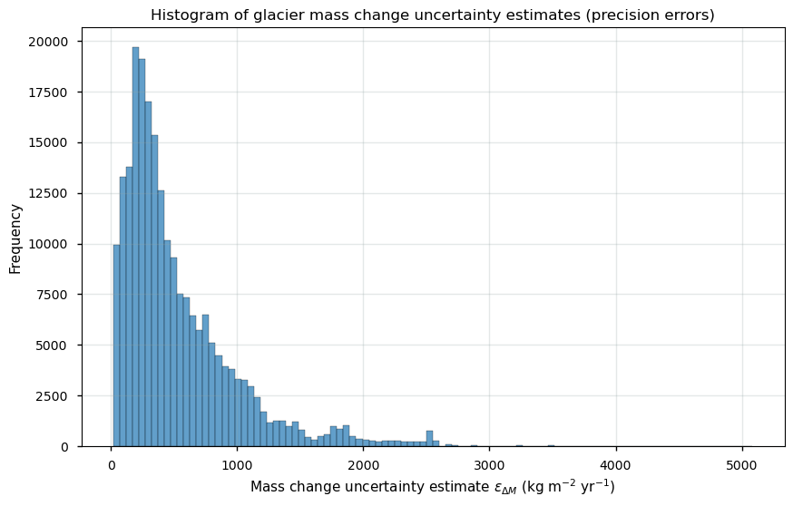
Figure 1. Histogram of pixel-by-pixel glacier mass change errors in the glacier mass change dataset.
Let us plot some statistics:
The overall arithmetic mean precision error over all pixels and all years is 530.69 kg m⁻² yr⁻¹ with a maximum of 5083.96 kg m⁻² yr⁻¹.
2.2 Glacier mass change errors over time#
The overall arithmetic mean error over both space and time exhibits a moderate magnitude, and the majority of errors seem to be situated close to 200-500 kg m⁻² yr⁻¹. The threshold (i.e. the minimum requirement to be met to ensure that data are useful) for glacier mass change uncertainty (expressed in terms of 2\(\sigma\)) proposed by the GCOS is 500 kg m⁻² yr⁻¹, while the “breakthrough” value (i.e. the level at which specified uses within climate monitoring become possible) would be 200 kg m⁻² yr⁻¹ per grid point [4].
As an extra step, we can calculate the overall arithmetic mean glacier mass change precision error for each hydrological year to get a general idea of the overall magnitude of the errors. This is simply calculated as the spatial arithmetic mean of all pixels for each year \(t\):
\(\overline{\varepsilon_{\Delta{M}}}_{x,y} \) [kg m⁻² yr⁻¹] \( = \dfrac{1}{n} \sum\limits^{{{x,y}}} (\varepsilon_{\Delta{M_{x,y}}})\) with \(x,y\) the spatial domain size and \(n\) is the total amount of latitude/longitude pixels (NaN pixels with no glaciers are excluded).
This results in the following:
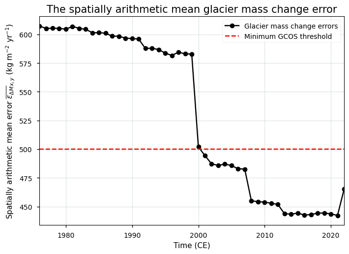
Figure 2. Time series of annual spatially averaged (arithmetic) glacier mass change errors in the glacier mass change dataset. The red dotted line represents the minimum uncertainty threshold proposed by GCOS [4].
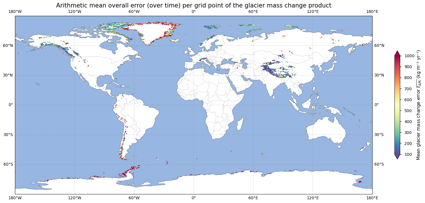
2.3 Glacier mass change errors in space#
Next, let us check the spatial distribution of the mean overall error over time per grid point, which is simply calculated as the temporal arithmetic mean over all years for each pixel \(x,y\):
\(\overline{\varepsilon_{\Delta{M_{t}}}} \) [kg m⁻² yr⁻¹] \( = \dfrac{1}{n} \sum\limits_{i={1976}}^{{{1976+n-1}}} (\varepsilon_{\Delta{M_i}})\) with \(n\) is the total amount of years in the time series.
This results in the following:
Let us make this plot a bit clearer by grouping these errors with respect to the threshold values proposed by GCOS [4]:
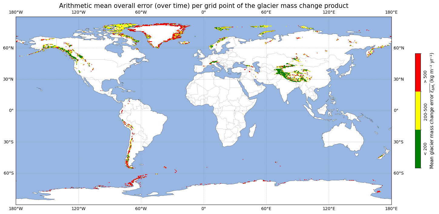
Green pixels indicate areas where the breakthrough value of (an uncertainty of 200 kg m⁻² yr⁻¹ or lower), as proposed by GCOS, has been reached, whereas red grid points exhibit temporally arithmetic mean error values that exceed the threshold value (500 kg m⁻² yr⁻¹ or more) for the data to be useful. This confirms our statement from above: especially the Greenland and Antarctic peripheral glaciers and parts of the Andes exhibit error values that are clearly too high. Extra care from the user is required in these regions since the threshold value has not been reached. Other regions, such as High Mountain Asia and the majority of Alaskan and European glaciers, have precision error values that allow for a reliable and high-quality data analysis. Possible reasons for this pattern are sparse data coverage, complex terrain, and gridded data limitations.
Let us quantify the percentage of data (over all pixels and all years) that do and do not reach the threshold values:
The percentage of data points with a glacier mass change error value less than 200 kg m⁻² yr⁻¹ is 21.79%.
The percentage of data points with a glacier mass change error value more than 500 kg m⁻² yr⁻¹ is 38.36%.
Now, let us plot the global annual mass change data over time and propagate its error throughout the time series.
3. Quantifying global (cumulative) glacier mass changes and their error estimates since 1975-1976#
3.1 Global glacier mass changes#
In the following section, we plot the global annual (and cumulative) glacier mass change over time. For the annual values, we therefore sum the gridded mass change product over the entire spatial domain for each individual year to get spatially summed values in Gt yr⁻¹, and calculate the glacier area-weighted mean to get a mass balance value in m w.e. yr⁻¹:
\(\Delta M_i \) [Gt yr⁻¹] \( = \sum\limits^{x,y}\Delta {M_{x,y,i}}\)
where \(\Delta {M_{x,y,i}}\) is the glacier mass change (from glacier_mass_change_gt, in Gt yr⁻¹) at pixel \(x,y\) during a certain year \(i\), and
\({\Delta B_i} \) [m w.e. yr⁻¹] \( = \textstyle\dfrac{1}{\sum\limits^{x,y} A_{x,y,i}} {\sum\limits^{x,y} (A_{x,y,i} * \Delta {B_{x,y,i}})}\)
where \(\Delta {B_{x,y,i}}\) is the glacier mass balance (from glacier_mass_change_mwe, in m w.e. yr⁻¹) and \(A_{x,y,i}\) the glacier area [km\(^2\)] at pixel \(x,y\) (from glacier_area_km2) during a certain year \(i\).
This results in the following plot:
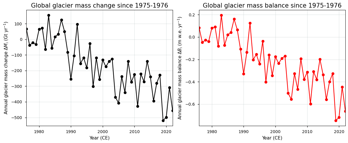
The mass changes in the left plot above are expressed in Gt yr\(^{-1}\) (Gigatonnes per year). Since Gt is a unit of mass, the mass of 1 Gt of ice is exactly the same as the mass of 1 Gt of water. The value can, however, also be translated into a volume. For example, 1 Gt of water (density 1000 kg/m³) is exactly 1 km³ water, while 1 Gt of ice (density 917 kg/m³) becomes 1.091 km³ of ice in volume.
3.2 Global glacier mass change error estimates#
By making use of the laws of error propagation, we can also determine how the glacier mass change errors propagate throughout the time series. For error propagation, we assume that:
Errors are spatially correlated within a certain RGI region, but are uncorrelated in between RGI regions
Errors are uncorrelated in time
The corresponding annual mass change uncertainty is calculated by assuming that errors are spatially correlated within a certain RGI region. To create the global error estimate, we assume uncorrelated/independent errors between the 19 RGI regions [2]. For error propagation, we also divide the uncertainty estimates by 1.96 since errors values are reported as 1.96 times the standard deviation in the original dataset:
\( \sigma_{\Delta{M_i}} \) [Gt yr⁻¹] \(= \sqrt{\sum\limits^{19}_{region=1}({\sigma_{ \Delta{M_{region,i}}}})^2} \) , where \( {\sigma_{ \Delta{M_{region,i}}}} = \sum\limits^{x,y \in \text{region}}({\sigma_{ \Delta{M_{x,y,i}}}}) \)
and \(\sigma_{ \Delta{M_{x,y,i}}}\) is the mass change standard deviation (from uncertainty_gt divided by 1.96, in Gt yr⁻¹) at pixel \(x,y\) during a certain year \(i\) in a certain RGI region, and
\( \sigma_{{\Delta{B_i}}} \) [m w.e. yr⁻¹] \(= \sqrt{\sum\limits^{19}_{region=1}({\sigma_{ \Delta{B_{region,i}}}})^2} \) , where \({\sigma_{ \Delta{B_{region,i}}}} = {\sum\limits^{x,y \in \text{region}} \left( \dfrac{A_{x,y,i}}{\sum\limits^{x,y \in \text{region}} A_{x,y,i}} * {\sigma_{{\Delta{B}_{x,y,i}}}} \right) } \)
where \(\sigma_{{ \Delta{B_{x,y,i}}}}\) is the mass balance standard deviation (from uncertainty_mwe divided by 1.96, in m w.e. yr⁻¹) at pixel \(x,y\) during a certain year \(i\) and \(A_{x,y,i}\) the glacier area [km\(^2\)] (from glacier_area_km2).
Plotting these data reveals the following:
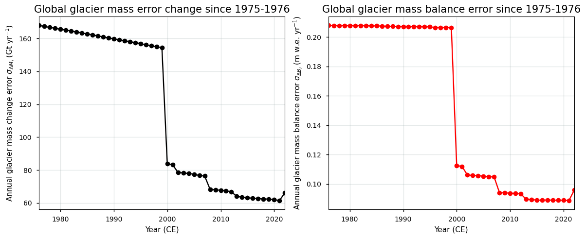
It can be seen from the plot that the global glacier mass change uncertainty has been decreasing over time, with a sudden drop around 2000 CE. The data can also be plotted in a cumulative way:
\( {M} \) [Gt] \( = \sum\limits_{i={1976}}^{{{1976+n-1}}} (\Delta M_i) \) , or
\( {{B}} \) [m w.e.] \( = \sum\limits_{i={1976}}^{{{1976+n-1}}} ({\Delta B_i}) \)
with the global annual glacier mass change (in Gt yr⁻¹) or balance (m w.e. yr⁻¹) at a certain year \(i\) (as calculated above) and \(n\) the number of years in the time series.
The corresponding uncertainty is calculated by assuming uncorrelated errors over time:
\( \sigma_{{M}} \) [Gt] \( = \sqrt{\sum\limits_{i={1976}}^{{1976+n-1}} (\sigma_{\Delta{M_i}})^2} \) , or
\( \sigma_{{{B}}} \) [m w.e.] = \( \sqrt{\sum\limits_{i={1976}}^{{1976+n-1}} (\sigma_{{\Delta{B_i}}})^2} \)
with the global annual mass change (in Gt yr⁻¹) or balance (m w.e. yr⁻¹) uncertainty at a certain year \(i\) (as calculated above) and \(n\) the number of years in the time series.
3.3 Time series of global cumulative glacier mass changes and their error estimate#
The corresponding plot looks as follows:
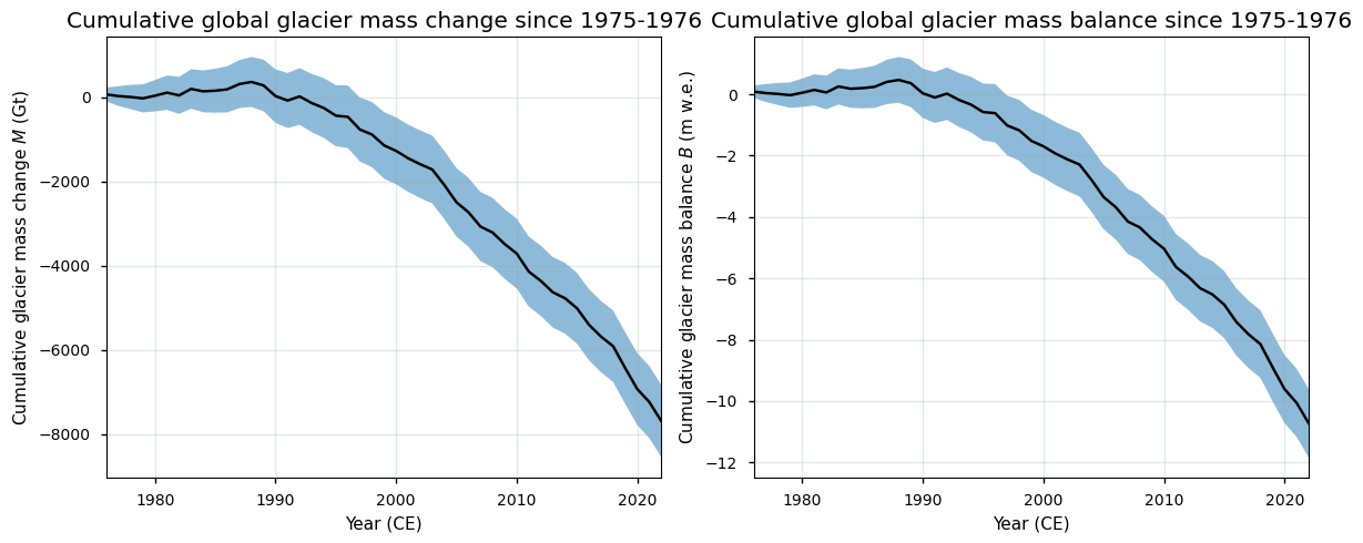
From the image above, it can be seen that glaciers clearly have been losing mass during the observational period, especially since the 1990s, which is in line with findings in the literature (e.g. [8]). The final estimate of the glaciers mass change at the end of the time series is:
The total global cumulative glacier mass change between 1975-1976 and 2021-2022 is -10.72 ± 1.12 m w.e. or -7691.70 ± 858.39 Gt.
Now, let us use the glacier mass change data to quantify the link between glacier melt and glacier-related contributions to global sea level rise in the context of Earth System modeling and climate change monitoring.
4. Quantification of glacier-related contributions to global sea level change#
4.1 Computing sea-level rise equivalent from glacier mass loss#
We can calculate the cumulative contribution of glacier mass changes to global sea level change during the last several decades by making use of the following formula [5]:
\( h_{SLE} \) [mm] \( = 1 \cdot 10^6 * \sum\limits_{i=1976}^{1976+n-1} \left(\dfrac{\Delta V_{i}}{A_s}\right) \)
where \( \Delta{V_{i}} = \dfrac{\rho_w}{\rho_s} * \sum\limits^{x,y}\left(\dfrac{\Delta {B_{x,y,i}}}{1 \cdot 10^3} * A_{x,y,i}\right) \).
Here, \(\Delta {B}\) is the glacier mass balance (in m w.e. yr⁻¹, divided by 1000 to get units in km) at pixel \(x,y\) during a certain year \(i\) from ds["glacier_mass_change_mwe"], and \(A\) the glacier area [km²] from ds["glacier_area_km2"], so that the annual volume change \(\Delta V\) has units of km\(^3\) yr\(^{-1}\) of water. Furthermore, \({A_{s}}\) is the ocean surface area [km²], \(n\) the total number of years in the time series and \(\rho\) the respective densities of water \(w\) and the sea \(s\) [kg m⁻³]. Note that this formulation assumes that all glacier mass or volume losses directly contribute to sea level changes, while this is not necessarily the case (e.g. [6, 7]). Also note that by multiplying the sea level contribution by \(\frac{\rho_w}{\rho_s}\), we calculate sea level contributions in ocean water column equivalent.
The corresponding uncertainty is given by:
\( \sigma_{h_{SLE}} \) [mm] = \( 1 \cdot 10^6 * \left(\dfrac{1}{A_s} \dfrac{{\rho_{w}}}{\rho_{s}}\right) * \sqrt{ \sum\limits_{i={1976}}^{{{1976+n-1}}} (\sigma_{{V_{i}}})^2} \)
where \(\sigma_{\Delta{V}}\) is the corresponding volume change uncertainty [km\(^{3}\) yr\(^{-1}\)] calculated from the mass balance uncertainty and the glacier area, again taking into account that uncertainties at the pixel level are given as 1.96 times the standard deviation and that errors within a certain RGI region are correlated, while uncorrelated between RGI regions and over time, as before.
4.2 Time series of glacier-related sea level contribution#
This ultimately results in the following graph:
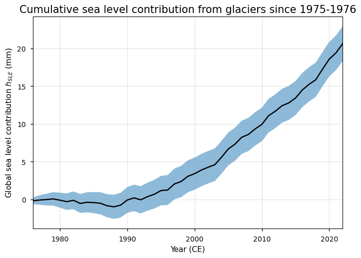
Figure 8. Cumulative contribution of glacier mass changes to global sea level changes (assuming all glacier mass changes contribute to sea level changes), including the propagation of the error (shaded).
Let us quantify the total glacier-related contribution to global sea level change since the beginning of the dataset:
The total contribution of glacier mass changes to global sea level change between 1975-1976 and 2021-2022 is 20.64 ± 2.30 mm.
The C3S product can be interpreted as glacier mass changes relevant for sea level contributions, as both the glaciological and geodetic approach do not consider ice melt that occurs under the waterline, which already displaces water. In contrast, processes that do contribute to sea level changes – such as liquid runoff from ice above buoyancy and changes in the ice flux across the grounding line – will result in a surface elevation change, which is observed with DEM differencing and hence incorporated in the geodetic method. Even though this consideration is not exact – a precise separation of contributions from ice above buoyancy (which affects sea level changes) and ice below buoyancy (which does not) would require the actual position of the grounding line, as well as values for the ice thickness and bedrock elevation field (e.g. [7]) – it is assumed that the resulting mass change estimates from this approach fall within acceptable uncertainty bounds to consider them relevant for sea level changes [2]. However, it should also be considered that not all mass changes affect sea levels directly, for example for landlocked glaciers whose meltwater does not reach the ocean [6, 7]).
5. Short summary and take-home messages#
To be able to use the glacier mass change dataset for reliable climate change analysis/monitoring purposes, the dataset should at least exhibit a comprehensive spatial coverage (i.e. global), a long and continuous temporal coverage (> 30 years), quantified and transparent pixel-by-pixel uncertainty estimates that meet international proposed thresholds [4], and an adequate spatio-temporal resolution (cfr. the “Maturity Matrix” [9]).
Since these conditions are generally met, the C3S glacier mass change dataset on the CDS is considered highly suitable for monitoring and deriving global cumulative mass changes over time, as well as assessing their impact on global sea level changes. The dataset, for example, includes pixel-by-pixel error estimates, expressed as precision errors (1.96 times the standard deviation). The corresponding uncertainty furthermore decreases over time, with post-2000 data meeting international GCOS standards. There is, however, a high spatial and temporal variation in the error estimates, implying that not all pixels meet these uncertainty thresholds. Users should therefore exercise caution in certain areas, such as the peripheral glaciers of Antarctica and Greenland, where uncertainties are higher. The dataset furthermore meets GCOS requirements in terms of resolution, spatial coverage (global) and temporal continuity (since 1975-76 without gaps), which demostrates its maturity and reliability for Earth system modeling and climate change monitoring. Data quality is hence considered strong, especially after 2000 and outside the high-uncertainty peripheral regions of the ice sheets.
The glacier mass change data can be considered to be directly transformable to sea level contributions, provided certain assumptions are made [2]. Additionally, users should note limitations, such as the absence of detailed sampling density information, the fact that data can not be consulted at the individual glacier-scale, and that data are measured and generated by different institutes/research groups and from different methods, which could result in inconsistencies. Moreover, since grid cells are not of the same absolute surface area and decrease in size at higher latitudes, mass change artefacts may arise in polar regions if individual glaciers are larger than the cell size. This may affect glacier mass change representativeness in some areas. Therefore, knowledge of the amount and spatial distribution of glaciers with a consistent and long-term glaciological sample is crucial for assessing the representativeness of the data.
ℹ️ If you want to know more#
Key resources#
Documentation on the CDS and the ECMWF Confluence Wiki (Copernicus Knowledge Base)
C3S EQC custom functions,
c3s_eqc_automatic_quality_controlprepared by B-Open
References#
[1] WGMS (2022). Fluctuations of Glaciers Database. doi: 10.5904/wgms-fog-2022-09.
[2] Dussaillant, I., Hugonnet, R., Huss, M., Berthier, E., Bannwart, J., Paul, F., and Zemp, M. (2025). Annual mass changes for each glacier in the world from 1976 to 2023, Earth Syst. Sci. Data, doi: 10.5194/essd-2024-323.
[3] Zemp, M., Huss, M., Thibert, E., Eckert, N., McNabb, R., Huber, J., Barandun, M., Machguth, H., Nussbaumer, S. U., Gärtner-Roer, I., Thomson, L., Paul, F., Maussion, F., Kutuzov, S., and Cogley, J. G. (2019). Global glacier mass changes and their contributions to sea-level rise from 1961 to 2016. Nature, 568, 382–386. doi: 10.1038/s41586-019-1071-0.
[4] GCOS (Global Climate Observing System) (2022). The 2022 GCOS ECVs Requirements (GCOS-245). World Meteorological Organization: Geneva, Switzerland. doi: https://library.wmo.int/idurl/4/58111
[5] Farinotti, D., Huss, M., Fürst, J. J., Landmann, J., Machguth, H., Maussion, F., and Pandit, A. (2019). A consensus estimate for the ice thickness distribution of all glaciers on Earth. Nature Geoscience, 12(3), 168-173. doi: 10.1038/s41561-019-0300-3.
[6] Bamber, J. L., Westaway, R. M., Marzeion, B., and Wouters, B. (2018): The land ice contribution to sea level during the satellite era. Environmental Research Letters, 13(6), 063008, doi: 10.1088/1748-9326/aac2f0.
[7] Goelzer, H., Coulon, V., Pattyn, F., de Boer, B., and van de Wal, R. (2020). Brief communication: On calculating the sea-level contribution in marine ice-sheet models, The Cryosphere, 14, 833–840, doi: 10.5194/tc-14-833-2020.
[8] The GlaMBIE Team (2025). Community estimate of global glacier mass changes from 2000 to 2023. Nature (2025). doi: 10.1038/s41586-024-08545-z.
[9] Yang, C. X., Cagnazzo, C., Artale, V., Nardelli, B. B., Buontempo, C., Busatto, J., Caporaso, L., Cesarini, C., Cionni, I., Coll, J., Crezee, B., Cristofanelli, P., de Toma, V., Essa, Y. H., Eyring, V., Fierli, F., Grant, L., Hassler, B., Hirschi, M., Huybrechts, P., Le Merle, E., Leonelli, F. E., Lin, X., Madonna, F., Mason, E., Massonnet, F., Marcos, M., Marullo, S., Muller, B., Obregon, A., Organelli, E., Palacz, A., Pascual, A., Pisano, A., Putero, D., Rana, A., Sanchez-Roman, A., Seneviratne, S. I., Serva, F., Storto, A., Thiery, W., Throne, P., Van Tricht, L., Verhaegen, Y., Volpe, G., and Santoleri, R. (2022). Independent Quality Assessment of Essential Climate Variables: Lessons Learned from the Copernicus Climate Change Service, B. Am. Meteorol. Soc., 103, E2032–E2049, doi: 10.1175/Bams-D-21-0109.1.