Please note that this repository is used for development and review, so quality assessments should be considered work in progress until they are merged into the main branch

7.1. Consistency between the C3S Atlas dataset and its origins: Case study

Production date: 2025-09-30.

Dataset version: 2.0.

Produced by: Olivier Burggraaff, Nicole Reynolds (National Physical Laboratory).

🌍 Use case: Retrieving climate indicators from the Copernicus Interactive Climate Atlas

❓ Quality assessment question

• Are the climate indicators in the dataset underpinning the Copernicus Interactive Climate Atlas consistent with their origin datasets?

• Can the dataset underpinning the Copernicus Interactive Climate Atlas be reproduced from its origin datasets?

The Copernicus Interactive Climate Atlas, or C3S Atlas for short, is a C3S web application providing an easy-to-access tool for exploring climate projections, reanalyses, and observational data [Gutiérrez+24]. Version 2.0 of the application allows the user to interact with 12 datasets:

Type	Dataset
Climate Projection	CMIP6
Climate Projection	CMIP5
Climate Projection	CORDEX-CORE
Climate Projection	CORDEX-EUR-11
Reanalysis	ERA5
Reanalysis	ERA5-Land
Reanalysis	ORAS5
Reanalysis	CERRA
Observations	E-OBS
Observations	BERKEARTH
Observations	CPC
Observations	SST-CCI

These datasets are provided through an intermediary dataset, the Gridded dataset underpinning the Copernicus Interactive Climate Atlas or C3S Atlas dataset for short [C3S Atlas dataset]. Compared to their origins, the versions of the climate datasets within the C3S Atlas dataset have been processed following the workflow in Figure 7.1.1.

Fig. 7.1.1 Schematic representation of the workflow for the production of the C3S Atlas dataset from its origin datasets, from the User-tools for the C3S Atlas.

Because a wide range of users interact with climate data through the C3S Atlas application, it is crucial that the underpinning dataset represent its origins correctly. In other words, the C3S Atlas dataset must be consistent with and reproducible from its origins. Here, we assess this consistency and reproducibility by comparing climate indicators retrieved from the C3S Atlas dataset with their equivalents calculated from the origin dataset, mirroring the workflow from Figure 7.1.1. While a full analysis and reproduction of every record within the C3S Atlas dataset is outside the scope of quality assessment (and would require high-performance computing infrastructure), a case study with a narrower scope probes these quality attributes of the dataset and can be a jumping-off point for further analysis by the reader.

This notebook is part of a series:

Notebook	Contents
Consistency between the C3S Atlas dataset and its origins: Case study	Comparison between C3S Atlas dataset and one origin dataset (CMIP6) for one indicator (tx35), including detailed setup.
Consistency between the C3S Atlas dataset and its origins: Multiple indicators	Comparison between C3S Atlas dataset and one origin dataset (CMIP6) for multiple indicators.
Consistency between the C3S Atlas dataset and its origins: Multiple origin datasets	Comparison between C3S Atlas dataset and multiple origin datasets for one indicator.

📢 Quality assessment statement

These are the key outcomes of this assessment

• Climate indicators (here tx35) provided by the C3S Atlas dataset are highly consistent with values calculated from its origin datasets (here the CMIP6 multi-model ensemble).

• Differences between the C3S Atlas dataset and a manual reproduction are rare (fewer than 0.1% of pixel pairs) and generally negligible (median absolute difference of 0).

• The C3S Atlas is traceable and reproducible, and can be confidently used to view, analyse, and download climate data.

📋 Methodology

This quality assessment tests the consistency between climate indicators retrieved from the Gridded dataset underpinning the Copernicus Interactive Climate Atlas [C3S Atlas dataset] and their equivalents calculated from the origin datasets, as well as the reproducibility of said dataset.

This notebook starts the quality assessment with a simple case study: one climate indicator derived from one origin dataset. This indicator is tx35, the Monthly count of days with maximum near-surface (2-metre) air temperature above 35 °C, derived from the CMIP6 multi-model ensemble [CMIP6 dataset]. This notebook mirrors one of the reproducibility demonstrations written by the data provider.

The analysis and results are organised in the following steps, which are detailed in the sections below:

1. Code setup

• Install User-tools for the C3S Atlas.

• Import all required libraries.

• Define indicator.

• Define helper functions.

2. Calculate indicator from the origin dataset

• Download data from the origin dataset.

• Homogenise data.

• Calculate indicator.

• Regrid the origin data to the C3S Atlas grid.

3. Retrieve indicator from the C3S Atlas dataset

• Download data from the C3S Atlas dataset.

4. Results

• Consistency: Compare the C3S Atlas and reproduced datasets on native grids.

• Reproducibility: Compare the C3S Atlas and reproduced datasets on the C3S Atlas grid.

📈 Analysis and results

1. Code setup

Note

This notebook uses earthkit for downloading (earthkit-data) and visualising (earthkit-plots) data. Because earthkit is in active development, some functionality may change after this notebook is published. If any part of the code stops functioning, please raise an issue on our GitHub repository so it can be fixed.

Install the User-tools for the C3S Atlas

This notebook uses the User-tools for the C3S Atlas, which can be installed from GitHub using pip. For convenience, the following cell can do this from within the notebook. Further details and alternative options for installing this library are available in its documentation.

Show code cell source

Hide code cell source

!pip install git+https://github.com/ecmwf-projects/c3s-atlas.git

Import required libraries

In this section, we import all the relevant packages needed for running the notebook.

Show code cell source

Hide code cell source

# Input / Output
from pathlib import Path
import earthkit.data as ekd
import warnings

# General data handling
import numpy as np
import pandas as pd
import xarray as xr
from functools import partial
from dask.array.core import PerformanceWarning
warnings.simplefilter(action="ignore", category=PerformanceWarning)

# Data pre-processing
from c3s_atlas.fixers import apply_fixers
import c3s_atlas.interpolation as xesmfCICA

# Climate indicators
import xclim

# Visualisation
import earthkit.plots as ekp
import matplotlib.pyplot as plt
plt.rcParams["grid.linestyle"] = "--"

# Visualisation in Jupyter book -- automatically ignored otherwise
try:
    from myst_nb import glue
except ImportError:
    glue = None

# Type hints
from typing import Iterable, Optional
from earthkit.plots.geo.domains import Domain
AnyDomain = (Domain | str)

Define indicators

This section defines functions and variables for calculating and using the climate indicators:

Show code cell source

Hide code cell source

# Functions to calculate indicators
def cal_tx35(ds: xr.Dataset) -> xr.Dataset:
    """ Monthly count of days with maximum near-surface (2-metre) air temperature above 35 °C """
    ds_tx35 = xclim.indices.tx_days_above(ds["tasmax"], thresh="35.0 degC", freq="MS", op=">").to_dataset(name="tx35")
    return ds_tx35

The following cell defines earthkit-plots styles for the indicators. These styles define the colour maps and colour bar ranges for each quantity. Earthkit-plots styles are explained further in the corresponding documentation.

Show code cell source

Hide code cell source

# Styles for indicators
n_diff = 5  # Levels in difference charts
_style_monthly_days      = {"vmin": 0,     "vmax": 30,    "extend": "neither"}
_style_monthly_days_diff = {"vmin": -2.5,  "vmax": 2.5,   "extend": "both"}
_style_tx35      = _style_monthly_days      | {"cmap": plt.cm.Oranges.resampled(10)}
_style_tx35_diff = _style_monthly_days_diff | {"cmap": plt.cm.RdBu_r.resampled(n_diff)}

styles = {
    "tx35":      ekp.styles.Style(**_style_tx35),
    "tx35_diff": ekp.styles.Style(**_style_tx35_diff),
}

# Apply general settings
for style in styles.values():
    style.normalize = False

Helper functions

This section defines some functions and variables used in the following analysis, allowing code cells in later sections to be shorter and ensuring consistency.

Data (pre-)processing

The following functions handle the homogenisation of origin data to a consistent format using the User-tools for the C3S Atlas:

Show code cell source

Hide code cell source

# Homogenisation of origin dataset
def homogenise(ds: xr.Dataset, var_name: str, project_id: str) -> xr.Dataset:
    """ Homogenise a dataset `ds` for one variable `var_name` """
    var_mapping = {
                "dataset_variable": {var_name: "data"},
                "aggregation": {"data": "mean"},
        }
    data = apply_fixers(ds, var_name, project_id, var_mapping)
    return data

# Homogenisation of origin dataset, multiple non-consecutive years
def homogenise_multiple_years(ds: xr.Dataset, var_name: str, project_id: str) -> xr.Dataset:
    """ Homogenise a dataset `ds` for one variable `var_name`, grouping over multiple years """
    homogenise_here = partial(homogenise, var_name=var_name, project_id=project_id)
    data = ds.groupby("time.year").map(homogenise_here)
    return data

The following functions handle regridding data based on ESMF as implemented in the User-tools for the C3S Atlas. This step is explained in more detail in the relevant section below.

Show code cell source

Hide code cell source

# Regridding from native grid to C3S Atlas grid
def regrid(ds: xr.Dataset, var_name: str) -> xr.Dataset:
    """ Regrid a dataset `ds` to the C3S Atlas grid for one variable `var_name` """
    int_attr = {"interpolation_method": "conservative_normed",
                "lats": np.arange(-89.5, 90.5, 1),
                "lons": np.arange(-179.5, 180.5, 1),
                "var_name": var_name,
    }
    INTER = xesmfCICA.Interpolator(int_attr)
    ds_interp = INTER(ds)
    return ds_interp

The following functions aid in sub-selecting data, e.g. selecting one model from the ensemble included in the C3S Atlas dataset or selecting data for a specific time frame:

Show code cell source

Hide code cell source

# C3S Atlas dataset: Individual model selection
def select_model_from_c3s_atlas_dataset(data: xr.Dataset, model: str) -> xr.Dataset:
    """ Select only data for the given model. """
    # Ensure the model ID is provided in the right format
    model_id = model.replace("_", "-")

    # Find the corresponding model ID in the list of models
    # This cannot use .sel because the coordinate is not indexed
    select_member = [str(mem) for mem in data.member_id.values if model_id in mem.lower()][0]

    # Find the corresponding data and return those
    member_ind = np.where(data.member_id == select_member)[0]
    data_member = data.sel(member=member_ind).squeeze("member")

    return data_member

# Select (multiple) years in a dataset
def select_years_in_dataset(data: xr.Dataset, years: list[int]) -> xr.Dataset:
    """ Select only data for the given year(s). """
    years_int = [int(y) for y in years]
    return data.sel(time=data.time.dt.year.isin(years_int))

# Select one month in multiple datasets
def select_month_in_multiple_datasets(*data: xr.Dataset, month: int) -> list[xr.Dataset]:
    """ Select only data for the given month, in any year. """
    data_month = [d.groupby("time.month")[month] for d in data]
    return data_month

Statistics

The following functions calculate the difference (absolute / relative) between datasets, handling metadata etc.:

Show code cell source

Hide code cell source

# Constants
NONZERO_THRESHOLD = 1e-5

# Difference between datasets
def difference_between_datasets(data1: xr.Dataset, data2: xr.Dataset, diff_variables: Iterable[str]) -> xr.Dataset:
    """ Calculate the difference between two datasets, preserving CRS and metadata. """
    # Subtract
    data1, data2 = [d.drop_vars(["lat_bnds", "lon_bnds", "time_bnds", "height"], errors="ignore") for d in (data1, data2)]
    difference = xr.ufuncs.subtract(data1, data2)
    return difference

def relative_difference_between_datasets(data1: xr.Dataset, data2: xr.Dataset, reldiff_variables: Iterable[str]) -> xr.Dataset:
    """
    Calculate the relative [%] difference between two datasets, preserving CRS and updating metadata.
    Relative difference is calculated relative to the first dataset.
    Where data1 == 0 and data2 == 0, the relative difference is set to 0 too.
    """
    # Select and calculate
    data1, data2 = [dataset.drop_vars([var for var in dataset.data_vars if var not in [*reldiff_variables, "crs"]]) \
                        for dataset in (data1, data2)]

    relative_difference = (data1 - data2) / data1 * 100.

    # Replace 0/0 with 0
    data1_zero = (data1 <= NONZERO_THRESHOLD)  # Threshold slightly > 0 because of floating-point errors
    relative_difference = relative_difference.where(~data1_zero, 0.)

    # Add name
    relative_difference = relative_difference.assign_attrs({"name": "C3S Atlas – Reproduced [%]"})

    return relative_difference

def fraction_over_threshold(data: pd.DataFrame, threshold: float=NONZERO_THRESHOLD) -> pd.DataFrame:
    """ Calculate the % of non-NaN cells in a dataframe greater than a given threshold. """
    data_over = (data >= threshold)
    frac_over = data_over.sum() / data_over.count() * 100.
    return frac_over

The following functions calculate and display metrics for the difference between two datasets, e.g. mean and median deviation:

Show code cell source

Hide code cell source

def comparison_statistics(dataset1: xr.Dataset, dataset2: xr.Dataset, indicator: str) -> pd.DataFrame:
    """
    Given two datasets, calculate a number of statistics for each variable and return the result in a table.
    `threshold` is used to determine values close to 0 (to within a float error).
    This version is hardcoded for one indicator in multiple years.
    """
    # Calculate differences
    differences     =          difference_between_datasets(dataset1, dataset2, diff_variables=[indicator])
    differences_rel = relative_difference_between_datasets(dataset1, dataset2, reldiff_variables=[indicator])

    # Convert to pandas
    differences = differences.to_dataframe()[[indicator]]
    differences_abs = differences.abs()

    differences_rel = differences_rel.to_dataframe()[[indicator]]
    differences_rel_abs = differences_rel.abs()

    # In this notebook: Group by year first
    differences, differences_abs, differences_rel, differences_rel_abs = [
        d.groupby(differences.index.get_level_values("time").year) for d in
        (differences, differences_abs, differences_rel, differences_rel_abs)
    ]

    # Calculate aggregate statistics
    md   =         differences.agg(["mean", "median"])  \
                              .rename(columns={"median": r"Median Δ", "mean": "Mean Δ"})
    mad  =     differences_abs.agg(["median"])  \
                              .rename(columns={"median": r"Median |Δ|"})
    mapd = differences_rel_abs.agg(["median"])  \
                              .rename(columns={"median": r"Median |Δ| [%]"})
    nonzero =  differences_abs.apply(fraction_over_threshold)  \
                              .rename(columns={indicator: r"% where |Δ| ≥ ε"})
    md, mad, mapd = [df.droplevel(0, axis=1) for df in (md, mad, mapd)]

    # Calculate correlation coefficients
    nr_years, data1_years, data2_years = _group_multiple_datasets_by_years(dataset1, dataset2)
    corrs = {year: xr.corr(d1[indicator], d2[indicator]).values
             for year, d1, d2 in _loop_over_data_grouped_by_year(data1_years, data2_years)}
    corrs = pd.DataFrame.from_dict(corrs, orient="index", columns=["Pearson r"])

    # Combine statistics into one dataframe
    stats = pd.concat([md, mad, nonzero, mapd, corrs], axis=1)

    return stats

def display_difference_stats(dataset1: xr.Dataset, dataset2: xr.Dataset, *args, **kwargs) -> str:
    """ Given two datasets, calculate a number of statistics for each variable and display the result in a table. """
    comparison_stats = comparison_statistics(dataset1, dataset2, *args, **kwargs)
    formatted = comparison_stats.style \
                                .format(precision=5)  \
                                .set_caption("C3S Atlas – Reproduced")
    return formatted

Visualisation

The following cells contain functions for plotting results, starting with some base helper functions (e.g. displaying in Jupyter Notebook or Jupyter Book style, adding textboxes with consistent formatting, etc.):

Show code cell source

Hide code cell source

# Visualisation: Helper functions, general
def _glue_or_show(fig: plt.Figure, glue_label: Optional[str]=None) -> None:
    """
    If `glue` is available, glue the figure using the provided label.
    If not, display the figure in the notebook.
    """
    try:
        glue(glue_label, fig, display=False)
    except TypeError:
        plt.show()
    finally:
        plt.close()

def _add_textbox_to_subplots(text: str, *axs: Iterable[plt.Axes | ekp.Subplot], right=False) -> None:
    """ Add a text box to each of the specified subplots. """
    # Get the plt.Axes for each ekp.Subplot
    axs = [subplot.ax if isinstance(subplot, ekp.Subplot) else subplot for subplot in axs]

    # Set up location
    x = 0.95 if right else 0.05
    horizontalalignment = "right" if right else "left"

    # Add the text
    for ax in axs:
        ax.text(x, 0.95, text, transform=ax.transAxes,
        horizontalalignment=horizontalalignment, verticalalignment="top",
        bbox={"facecolor": "white", "edgecolor": "black", "boxstyle": "round",
              "alpha": 1})

def _sharexy(axs: np.ndarray) -> None:
    """ Force all of the axes in axs to share x and y with the first element. """
    main_ax = axs.ravel()[0]
    for ax in axs.ravel():
        ax.sharex(main_ax)
        ax.sharey(main_ax)

def _symmetric_xlim(ax: plt.Axes) -> None:
    """ Adjust the xlims for one Axes to be symmetric, based on existing values. """
    current = ax.get_xlim()
    current = np.abs(current)
    maxlim = np.max(current)
    newlim = (-maxlim, maxlim)

    ax.set_xlim(newlim)

The following functions are also base helper functions, but specific to geospatial plots:

Show code cell source

Hide code cell source

# Visualisation: Helper functions for geospatial plots
def _spatial_plot_append_subplots(fig: ekp.Figure, *data: xr.Dataset, domain: Optional[AnyDomain]=None, **kwargs) -> list[ekp.Subplot]:
    """ Plot any number of datasets into new subplots in an existing earthkit figure. """
    # Create subplots
    subplots = [fig.add_map(domain=domain) for d in data]

    # Plot
    for subplot, d in zip(subplots, data):
        subplot.grid_cells(d, **kwargs)

    return subplots

def _group_multiple_datasets_by_years(*data: xr.Dataset) -> tuple[int, xr.core.groupby.GroupBy]:
    """ Apply groupby("time.year") to multiple datasets, return these, and return the number of years. """
    data_by_year = [d.groupby("time.year") for d in data]
    nr_years = len(data_by_year[0])
    return nr_years, *data_by_year

def _loop_over_data_grouped_by_year(data1: xr.core.groupby.GroupBy, data2: xr.core.groupby.GroupBy):
    """ Generator to more easily loop over multiple datasets that have been grouped by year. """
    for (year, d1), (_, d2) in zip(data1, data2):
        # Remove redundant time coordinate
        d1, d2 = [d.drop_vars("time") for d in (d1, d2)]

        yield (year, d1, d2)

The following cell contains functions for geospatial comparisons between datasets on their native grids or on a common grid (the latter also showing the per-pixel difference):

Show code cell source

Hide code cell source

# Visualisation: Plot indicators geospatially
def geospatial_comparison(data1: xr.Dataset, data2: xr.Dataset, indicator: str, month: int, *,
                          label1: str="C3S Atlas dataset", label2: str="Reproduced from origin",
                          domain: Optional[AnyDomain]=None,
                          glue_label: Optional[str]=None) -> ekp.Figure:
    """
    Plot one indicator in two datasets.
    If multiple years are present, loops over those using groupby.
    A specific month has to be specified.
    """
    # Pre-process: Select data in one month, group by year
    data_by_month = select_month_in_multiple_datasets(data1, data2, month=month)
    nr_years, data1_years, data2_years = _group_multiple_datasets_by_years(*data_by_month)

    # Create figure
    fig = ekp.Figure(rows=nr_years, columns=2, size=(8, 4*nr_years))

    # Plot indicators
    for year, d1, d2 in _loop_over_data_grouped_by_year(data1_years, data2_years):
        # Plot individual datasets
        subplots_data = _spatial_plot_append_subplots(fig, d1, d2, domain=domain, z=indicator, style=styles[indicator])

        # Decorate: Text + Colour bar
        _add_textbox_to_subplots(year, *subplots_data)
        subplots_data[-1].legend(label=indicator, location="right")

    # Titles on top
    titles = [label1, label2]
    for title, subplot in zip(titles, fig.subplots):
        subplot.ax.set_title(title)

    # Decorate figure
    fig.land()
    fig.coastlines()
    fig.gridlines(linestyle=plt.rcParams["grid.linestyle"])

    # Show result
    _glue_or_show(fig.fig, glue_label)


# Visualisation: Plot indicator + difference geospatially
def geospatial_comparison_with_difference(data1: xr.Dataset, data2: xr.Dataset, indicator: str, month: int, *,
                                          label1: str="C3S Atlas dataset", label2: str="Reproduced from origin",
                                          domain: Optional[AnyDomain]=None,
                                          glue_label: Optional[str]=None) -> ekp.Figure:
    """
    Plot one indicator in two datasets, including the difference between them.
    If multiple years are present, loops over those using groupby.
    A specific month has to be specified.
        TO DO: glue
    """
    # Pre-process: Select data in one month, group by year
    data_by_month = select_month_in_multiple_datasets(data1, data2, month=month)
    nr_years, data1_years, data2_years = _group_multiple_datasets_by_years(*data_by_month)

    # Create figure
    fig = ekp.Figure(rows=nr_years, columns=3, size=(8, 3*nr_years))

    # Plot indicators
    for year, d1, d2 in _loop_over_data_grouped_by_year(data1_years, data2_years):
        # Plot individual datasets
        subplots_data = _spatial_plot_append_subplots(fig, d1, d2, domain=domain, z=indicator, style=styles[indicator])

        # Plot difference
        difference = difference_between_datasets(d1, d2, diff_variables=[indicator])
        subplot_diff = fig.add_map(domain=domain)
        subplot_diff.grid_cells(difference, z=indicator, style=styles[f"{indicator}_diff"])

        # Show year
        _add_textbox_to_subplots(year, *subplots_data, subplot_diff)

    # Colour bar at the bottom
    for subplot in subplots_data:
        subplot.legend(label=indicator, location="bottom")
    subplot_diff.legend(label="Difference", location="bottom")

    # Titles on top
    titles = [label1, label2, "Difference"]
    for title, subplot in zip(titles, fig.subplots):
        subplot.ax.set_title(title)

    # Decorate figure
    fig.land()
    fig.coastlines()
    fig.gridlines(linestyle=plt.rcParams["grid.linestyle"])

    # Show result
    _glue_or_show(fig.fig, glue_label)

The following cell contains functions for histogram comparisons between datasets on their native grids or on a common grid (the latter also showing the per-pixel difference):

Show code cell source

Hide code cell source

# Visualisation: Plot data in histograms
def histogram_comparison_by_year(data1: xr.Dataset, data2: xr.Dataset, indicator: str, *,
                                 label1: str="C3S Atlas dataset", label2: str="Reproduced from origin",
                                 glue_label: Optional[str]=None) -> plt.Figure:
    """
    Create a histogram for one indicator in two datasets, for multiple years.
    Flattens all data in the datasets, including spatial and temporal dimensions.
        TO DO: glue
    """
    # Group data by year
    nr_years, data1_years, data2_years = _group_multiple_datasets_by_years(data1, data2)

    # Create figure
    fig, axs = plt.subplots(nrows=nr_years, ncols=2, sharex=True, sharey=True,
                            figsize=(5, 2*nr_years), layout="constrained", squeeze=False)

    # Plot histograms of data
    # Loop over rows / indicators
    for ax_row, (year, d1, d2) in zip(axs, _loop_over_data_grouped_by_year(data1_years, data2_years)):
        # Loop over columns / data
        for ax, data in zip(ax_row, (d1, d2)):
            # Flatten data
            d = data[indicator].values.ravel()

            # Create histogram
            ax.hist(d, bins=31, density=True, log=True, color="black")

            # Labels
            ax.grid(True, axis="both")
            ax.set_xlabel(indicator)

        ax_row[0].set_ylabel("Frequency")

        # Identify panel
        _add_textbox_to_subplots(year, *ax_row, right=True)

    # Titles on top
    titles = [label1, label2]
    for title, ax in zip(titles, axs[0]):
        ax.set_title(title)

    # Show result
    _glue_or_show(fig, glue_label)


# Visualisation: Plot data + difference in histograms
def histogram_comparison_by_year_with_difference(data1: xr.Dataset, data2: xr.Dataset, indicator: str, *,
                                                 label1: str="C3S Atlas dataset", label2: str="Reproduced from origin",
                                                 glue_label: Optional[str]=None) -> plt.Figure:
    """
    Create a histogram for one indicator in two datasets, for multiple years, including the point-by-point difference.
    Flattens all data in the datasets, including spatial and temporal dimensions.
        TO DO: glue
    """
    # Group data by year
    nr_years, data1_years, data2_years = _group_multiple_datasets_by_years(data1, data2)

    # Create figure
    fig, axs = plt.subplots(nrows=nr_years, ncols=3,
                            figsize=(8, 2*nr_years), layout="constrained", squeeze=False)

    # Setup x/y share -- cannot be done in plt.subplots because of difference panel not sharing these
    _sharexy(axs[:, :-1])
    _sharexy(axs[:, -1])

    for ax in axs[:-1].ravel():
        ax.tick_params(axis="x", labelbottom=False)
        ax.xaxis.label.set_visible(False)

    for ax in axs[:, 1:-1].ravel():
        ax.tick_params(axis="y", labelleft=False)

    for ax in axs[:, -1].ravel():
        ax.yaxis.set_label_position("right")
        ax.tick_params(axis="y", labelleft=False, labelright=True)

    # Plot histograms of data
    # Loop over rows / indicators
    for ax_row, (year, d1, d2) in zip(axs, _loop_over_data_grouped_by_year(data1_years, data2_years)):
        # Calculate difference
        difference = difference_between_datasets(d1, d2, diff_variables=[indicator])

        # Loop over columns / data
        for ax, data in zip(ax_row, (d1, d2)):
            # Flatten data
            d = data[indicator].values.ravel()

            # Create histogram
            ax.hist(d, bins=31, density=True, log=True, color="black")

            # Labels
            ax.grid(True, axis="both")
            ax.set_xlabel(indicator)

            # Plot difference
            difference_here = difference[indicator].values.ravel()
            ax_row[-1].hist(difference_here, bins=31, density=True, log=True, color="black")

        ax_row[0].set_ylabel("Frequency")

        # Identify panel
        _add_textbox_to_subplots(year, *ax_row, right=True)

    for ax in axs[:, -1]:  # Symmetric xlims for difference
        _symmetric_xlim(ax)

    # Titles on top
    titles = [label1, label2, "Difference"]
    for title, ax in zip(titles, axs[0]):
        ax.set_title(title)

    # Decorate figure
    axs[-1, -1].set_xlabel("Difference")

    # Show result
    _glue_or_show(fig, glue_label)

2. Calculate indicator from the origin dataset

Download data

This assessment examines the dataset in two years (2060 and 2080), for one ensemble member and for one climate scenario – which is not how climate projection data are normally used. Good practice in climate science is to look at multi-year statistics and trends, across multiple ensemble members. However, since the purpose of this assessment is to assess the consistency and reproducibility of the post-processing performed to produce the C3S Atlas dataset, it is valid to use a subset of the data here. The specific subset used can be easily tweaked by changing the EXPERIMENT, MODEL, and YEARS variables in this section.

This notebook uses earthkit-data to download files from the CDS. If you intend to run this notebook multiple times, it is highly recommended that you enable caching to prevent having to download the same files multiple times. If you prefer not to use earthkit, the following requests can also be used with the cdsapi module. In either case (earthkit-data or cdsapi), it is required to set up a CDS account and API key as explained on the CDS website.

The first step is to define the parameters that will be shared between the download of the origin dataset (here CMIP6) and the C3S Atlas dataset (in the next section), namely the experiment and model member. Next, the request to download the corresponding data from CMIP6 is defined, in this notebook choosing only the variable necessary to calculate the tx35 indicator, namely daily_maximum_near_surface_air_temperature. Because the indicator will be calculated for multiple years, the year parameter of the request is left out for now.

Show code cell source

Hide code cell source

indicator = "tx35"

# Define request
ORIGIN_ID = "projections-cmip6"
ORIGIN = "cmip6"  # Used in C3S Atlas download; defined here to improve customisability
EXPERIMENT = "ssp5_8_5"
MODEL = "cmcc_esm2"

request_cmip6 = {
    "experiment": EXPERIMENT,
    "model": MODEL,
    "variable": "daily_maximum_near_surface_air_temperature",
    "temporal_resolution": "daily",
    "month": [f"{month:02d}" for month in range(1, 13)],
    "day": [f"{day:02d}" for day in range(1, 32)],
    "format": "netcdf",
}

This case study examines two years, namely 2060 and 2080, so there are two corresponding requests. This can easily be changed or extended to use different years. Separate requests are defined for each year, rather than one combined request, to limit the size per request.

Show code cell source

Hide code cell source

YEARS = [2060, 2080]
requests_year = [{"year": str(year)} for year in YEARS]

Show code cell source

Hide code cell source

requests_cmip6_combined = [request_cmip6 | req_year for req_year in requests_year]

# Download data
ds_cmip6 = ekd.from_source("cds", ORIGIN_ID, *requests_cmip6_combined)

Earthkit downloads the data as a field list. This is converted into an xarray dataset, which can be used in the following analysis.

Show code cell source

Hide code cell source

data_cmip6 = ds_cmip6.to_xarray(compat="equals", data_vars="all")
data_cmip6

<xarray.Dataset> Size: 167MB
Dimensions:    (time: 730, bnds: 2, lat: 192, lon: 288)
Coordinates:
  * time       (time) object 6kB 2060-01-01 12:00:00 ... 2080-12-31 12:00:00
  * lat        (lat) float64 2kB -90.0 -89.06 -88.12 -87.17 ... 88.12 89.06 90.0
  * lon        (lon) float64 2kB 0.0 1.25 2.5 3.75 ... 355.0 356.2 357.5 358.8
    height     float64 8B 2.0
Dimensions without coordinates: bnds
Data variables:
    time_bnds  (time, bnds) object 12kB dask.array<chunksize=(1, 2), meta=np.ndarray>
    lat_bnds   (time, lat, bnds) float64 2MB dask.array<chunksize=(365, 192, 2), meta=np.ndarray>
    lon_bnds   (time, lon, bnds) float64 3MB dask.array<chunksize=(365, 288, 2), meta=np.ndarray>
    tasmax     (time, lat, lon) float32 161MB dask.array<chunksize=(1, 192, 288), meta=np.ndarray>
Attributes: (12/48)
    Conventions:            CF-1.7 CMIP-6.2
    activity_id:            ScenarioMIP
    branch_method:          standard
    branch_time_in_child:   60225.0
    branch_time_in_parent:  60225.0
    comment:                none
    ...                     ...
    title:                  CMCC-ESM2 output prepared for CMIP6
    variable_id:            tasmax
    variant_label:          r1i1p1f1
    license:                CMIP6 model data produced by CMCC is licensed und...
    cmor_version:           3.6.0
    tracking_id:            hdl:21.14100/a1513d6f-5325-4b99-bbe6-9b096557b100

xarray.Dataset

• Dimensions:
  • time: 730
  • bnds: 2
  • lat: 192
  • lon: 288
• Coordinates: (4)
  • time
    (time)
    object
    2060-01-01 12:00:00 ... 2080-12-...

    bounds :

    time_bnds

    axis :

    T

    long_name :

    time

    standard_name :

    time

    array([cftime.DatetimeNoLeap(2060, 1, 1, 12, 0, 0, 0, has_year_zero=True),
           cftime.DatetimeNoLeap(2060, 1, 2, 12, 0, 0, 0, has_year_zero=True),
           cftime.DatetimeNoLeap(2060, 1, 3, 12, 0, 0, 0, has_year_zero=True), ...,
           cftime.DatetimeNoLeap(2080, 12, 29, 12, 0, 0, 0, has_year_zero=True),
           cftime.DatetimeNoLeap(2080, 12, 30, 12, 0, 0, 0, has_year_zero=True),
           cftime.DatetimeNoLeap(2080, 12, 31, 12, 0, 0, 0, has_year_zero=True)],
          shape=(730,), dtype=object)

  • lat
    (lat)
    float64
    -90.0 -89.06 -88.12 ... 89.06 90.0

    bounds :

    lat_bnds

    units :

    degrees_north

    axis :

    Y

    long_name :

    Latitude

    standard_name :

    latitude

    array([-90.      , -89.057592, -88.115183, -87.172775, -86.230366, -85.287958,
           -84.34555 , -83.403141, -82.460733, -81.518325, -80.575916, -79.633508,
           -78.691099, -77.748691, -76.806283, -75.863874, -74.921466, -73.979058,
           -73.036649, -72.094241, -71.151832, -70.209424, -69.267016, -68.324607,
           -67.382199, -66.439791, -65.497382, -64.554974, -63.612565, -62.670157,
           -61.727749, -60.78534 , -59.842932, -58.900524, -57.958115, -57.015707,
           -56.073298, -55.13089 , -54.188482, -53.246073, -52.303665, -51.361257,
           -50.418848, -49.47644 , -48.534031, -47.591623, -46.649215, -45.706806,
           -44.764398, -43.82199 , -42.879581, -41.937173, -40.994764, -40.052356,
           -39.109948, -38.167539, -37.225131, -36.282723, -35.340314, -34.397906,
           -33.455497, -32.513089, -31.570681, -30.628272, -29.685864, -28.743455,
           -27.801047, -26.858639, -25.91623 , -24.973822, -24.031414, -23.089005,
           -22.146597, -21.204188, -20.26178 , -19.319372, -18.376963, -17.434555,
           -16.492147, -15.549738, -14.60733 , -13.664921, -12.722513, -11.780105,
           -10.837696,  -9.895288,  -8.95288 ,  -8.010471,  -7.068063,  -6.125654,
            -5.183246,  -4.240838,  -3.298429,  -2.356021,  -1.413613,  -0.471204,
             0.471204,   1.413613,   2.356021,   3.298429,   4.240838,   5.183246,
             6.125654,   7.068063,   8.010471,   8.95288 ,   9.895288,  10.837696,
            11.780105,  12.722513,  13.664921,  14.60733 ,  15.549738,  16.492147,
            17.434555,  18.376963,  19.319372,  20.26178 ,  21.204188,  22.146597,
            23.089005,  24.031414,  24.973822,  25.91623 ,  26.858639,  27.801047,
            28.743455,  29.685864,  30.628272,  31.570681,  32.513089,  33.455497,
            34.397906,  35.340314,  36.282723,  37.225131,  38.167539,  39.109948,
            40.052356,  40.994764,  41.937173,  42.879581,  43.82199 ,  44.764398,
            45.706806,  46.649215,  47.591623,  48.534031,  49.47644 ,  50.418848,
            51.361257,  52.303665,  53.246073,  54.188482,  55.13089 ,  56.073298,
            57.015707,  57.958115,  58.900524,  59.842932,  60.78534 ,  61.727749,
            62.670157,  63.612565,  64.554974,  65.497382,  66.439791,  67.382199,
            68.324607,  69.267016,  70.209424,  71.151832,  72.094241,  73.036649,
            73.979058,  74.921466,  75.863874,  76.806283,  77.748691,  78.691099,
            79.633508,  80.575916,  81.518325,  82.460733,  83.403141,  84.34555 ,
            85.287958,  86.230366,  87.172775,  88.115183,  89.057592,  90.      ])

  • lon
    (lon)
    float64
    0.0 1.25 2.5 ... 356.2 357.5 358.8

    bounds :

    lon_bnds

    units :

    degrees_east

    axis :

    X

    long_name :

    Longitude

    standard_name :

    longitude

    array([  0.  ,   1.25,   2.5 , ..., 356.25, 357.5 , 358.75], shape=(288,))

  • height
    ()
    float64
    2.0

    units :

    m

    axis :

    Z

    positive :

    up

    long_name :

    height

    standard_name :

    height

    array(2.)

• Data variables: (4)
  • time_bnds
    (time, bnds)
    object
    dask.array<chunksize=(1, 2), meta=np.ndarray>

    Array Chunk Bytes 11.41 kiB 16 B Shape (730, 2) (1, 2) Dask graph 730 chunks in 5 graph layers Data type object numpy.ndarray

  • lat_bnds
    (time, lat, bnds)
    float64
    dask.array<chunksize=(365, 192, 2), meta=np.ndarray>

    Array Chunk Bytes 2.14 MiB 1.07 MiB Shape (730, 192, 2) (365, 192, 2) Dask graph 2 chunks in 7 graph layers Data type float64 numpy.ndarray

  • lon_bnds
    (time, lon, bnds)
    float64
    dask.array<chunksize=(365, 288, 2), meta=np.ndarray>

    Array Chunk Bytes 3.21 MiB 1.60 MiB Shape (730, 288, 2) (365, 288, 2) Dask graph 2 chunks in 7 graph layers Data type float64 numpy.ndarray

  • tasmax
    (time, lat, lon)
    float32
    dask.array<chunksize=(1, 192, 288), meta=np.ndarray>

    standard_name :

    air_temperature

    long_name :

    Daily Maximum Near-Surface Air Temperature

    comment :

    maximum near-surface (usually, 2 meter) air temperature (add cell_method attribute 'time: max')

    units :

    K

    original_name :

    TREFHTMX

    cell_methods :

    area: mean time: maximum

    cell_measures :

    area: areacella

    history :

    2021-01-18T14:11:28Z altered by CMOR: Treated scalar dimension: 'height'.

    Array Chunk Bytes 153.98 MiB 216.00 kiB Shape (730, 192, 288) (1, 192, 288) Dask graph 730 chunks in 5 graph layers Data type float32 numpy.ndarray

• Indexes: (3)
  • time
    PandasIndex

    PandasIndex(CFTimeIndex([2060-01-01 12:00:00, 2060-01-02 12:00:00, 2060-01-03 12:00:00,
                 2060-01-04 12:00:00, 2060-01-05 12:00:00, 2060-01-06 12:00:00,
                 2060-01-07 12:00:00, 2060-01-08 12:00:00, 2060-01-09 12:00:00,
                 2060-01-10 12:00:00,
                 ...
                 2080-12-22 12:00:00, 2080-12-23 12:00:00, 2080-12-24 12:00:00,
                 2080-12-25 12:00:00, 2080-12-26 12:00:00, 2080-12-27 12:00:00,
                 2080-12-28 12:00:00, 2080-12-29 12:00:00, 2080-12-30 12:00:00,
                 2080-12-31 12:00:00],
                dtype='object', length=730, calendar='noleap', freq=None))

  • lat
    PandasIndex

    PandasIndex(Index([             -90.0, -89.05759162303664,  -88.1151832460733,
           -87.17277486910994,  -86.2303664921466, -85.28795811518324,
            -84.3455497382199, -83.40314136125654, -82.46073298429319,
           -81.51832460732984,
           ...
            81.51832460732984,   82.4607329842932,  83.40314136125653,
            84.34554973821989,  85.28795811518324,   86.2303664921466,
            87.17277486910996,  88.11518324607329,  89.05759162303664,
                         90.0],
          dtype='float64', name='lat', length=192))

  • lon
    PandasIndex

    PandasIndex(Index([   0.0,   1.25,    2.5,   3.75,    5.0,   6.25,    7.5,   8.75,   10.0,
            11.25,
           ...
            347.5, 348.75,  350.0, 351.25,  352.5, 353.75,  355.0, 356.25,  357.5,
           358.75],
          dtype='float64', name='lon', length=288))

• Attributes: (48)

  Conventions :

  CF-1.7 CMIP-6.2

  activity_id :

  ScenarioMIP

  branch_method :

  standard

  branch_time_in_child :

  60225.0

  branch_time_in_parent :

  60225.0

  comment :

  none

  contact :

  T. Lovato

  creation_date :

  2021-01-18T14:12:06Z

  data_specs_version :

  01.00.31

  experiment :

  update of RCP8.5 based on SSP5

  experiment_id :

  ssp585

  external_variables :

  areacella

  forcing_index :

  1

  frequency :

  day

  further_info_url :

  https://furtherinfo.es-doc.org/CMIP6.CMCC.CMCC-ESM2.ssp585.none.r1i1p1f1

  grid :

  native atmosphere regular grid

  grid_label :

  gn

  history :

  2021-01-18T14:12:06Z ;rewrote data to be consistent with ScenarioMIP for variable tasmax found in table day.; none

  initialization_index :

  1

  institution :

  Fondazione Centro Euro-Mediterraneo sui Cambiamenti Climatici, Lecce 73100, Italy

  institution_id :

  CMCC

  mip_era :

  CMIP6

  nominal_resolution :

  100 km

  parent_activity_id :

  CMIP

  parent_experiment_id :

  historical

  parent_mip_era :

  CMIP6

  parent_source_id :

  CMCC-ESM2

  parent_time_units :

  days since 1850-01-01

  parent_variant_label :

  r1i1p1f1

  physics_index :

  1

  product :

  model-output

  realization_index :

  1

  realm :

  atmos

  references :

  none

  run_variant :

  1st realization

  source :

  CMCC-ESM2 (2017): aerosol: MAM3 atmos: CAM5.3 (1deg; 288 x 192 longitude/latitude; 30 levels; top at ~2 hPa) atmosChem: none land: CLM4.5 (BGC mode) landIce: none ocean: NEMO3.6 (ORCA1 tripolar primarly 1 deg lat/lon with meridional refinement down to 1/3 degree in the tropics; 362 x 292 longitude/latitude; 50 vertical levels; top grid cell 0-1 m) ocnBgchem: BFM5.1 seaIce: CICE4.0

  source_id :

  CMCC-ESM2

  source_type :

  AOGCM BGC

  sub_experiment :

  none

  sub_experiment_id :

  none

  table_id :

  day

  table_info :

  Creation Date:(05 February 2020) MD5:6a248fd76c55aa6d6f7b3cc6866b5faf

  title :

  CMCC-ESM2 output prepared for CMIP6

  variable_id :

  tasmax

  variant_label :

  r1i1p1f1

  license :

  CMIP6 model data produced by CMCC is licensed under a Creative Commons Attribution ShareAlike 4.0 International License (https://creativecommons.org/licenses). Consult https://pcmdi.llnl.gov/CMIP6/TermsOfUse for terms of use governing CMIP6 output, including citation requirements and proper acknowledgment. Further information about this data, including some limitations, can be found via the further_info_url (recorded as a global attribute in this file) and at https:///pcmdi.llnl.gov/. The data producers and data providers make no warranty, either express or implied, including, but not limited to, warranties of merchantability and fitness for a particular purpose. All liabilities arising from the supply of the information (including any liability arising in negligence) are excluded to the fullest extent permitted by law.

  cmor_version :

  3.6.0

  tracking_id :

  hdl:21.14100/a1513d6f-5325-4b99-bbe6-9b096557b100

Homogenise data

One of the steps in the C3S Atlas dataset production chain is homogenisation, i.e. ensuring consistency between data from different origin datasets. This homogenisation is implemented in the User-tools for the C3S Atlas, specifically the c3s_atlas.fixers.apply_fixers function. The following changes are applied:

• The names of the spatial coordinates are standardised to [lon, lat].

• Longitude is converted from [0...360] to [-180...180] format.

• The time coordinate is standardised to the CF standard calendar.

• Variable units are standardised (e.g. °C for temperature).

• Variables are resampled / aggregated to the required temporal resolution.

The homogenisation is applied in the following code cell. The apply_fixers function describes the different homogenisation steps as it applies them; this can be read by expanding the following cell outputs.

Show code cell source

Hide code cell source

VARIABLE = "tasmax"
data_cmip6_homogenised = homogenise_multiple_years(data_cmip6, var_name=VARIABLE, project_id=ORIGIN)

Show code cell output

Hide code cell output

2025-09-30 20:57:27,598 — Homogenization-fixers — INFO — Dataset has already the correct names for its coordinates
2025-09-30 20:57:27,609 — Homogenization-fixers — INFO — Fixing calendar for <xarray.Dataset> Size: 84MB
Dimensions:    (time: 365, bnds: 2, lat: 192, lon: 288)
Coordinates:
  * time       (time) object 3kB 2060-01-01 12:00:00 ... 2060-12-31 12:00:00
  * lat        (lat) float64 2kB -90.0 -89.06 -88.12 -87.17 ... 88.12 89.06 90.0
  * lon        (lon) float64 2kB 0.0 1.25 2.5 3.75 ... 355.0 356.2 357.5 358.8
    height     float64 8B 2.0
Dimensions without coordinates: bnds
Data variables:
    time_bnds  (time, bnds) object 6kB dask.array<chunksize=(1, 2), meta=np.ndarray>
    lat_bnds   (time, lat, bnds) float64 1MB dask.array<chunksize=(365, 192, 2), meta=np.ndarray>
    lon_bnds   (time, lon, bnds) float64 2MB dask.array<chunksize=(365, 288, 2), meta=np.ndarray>
    tasmax     (time, lat, lon) float32 81MB dask.array<chunksize=(1, 192, 288), meta=np.ndarray>
Attributes: (12/48)
    Conventions:            CF-1.7 CMIP-6.2
    activity_id:            ScenarioMIP
    branch_method:          standard
    branch_time_in_child:   60225.0
    branch_time_in_parent:  60225.0
    comment:                none
    ...                     ...
    title:                  CMCC-ESM2 output prepared for CMIP6
    variable_id:            tasmax
    variant_label:          r1i1p1f1
    license:                CMIP6 model data produced by CMCC is licensed und...
    cmor_version:           3.6.0
    tracking_id:            hdl:21.14100/a1513d6f-5325-4b99-bbe6-9b096557b100
2025-09-30 20:57:27,877 — UNITS_TRANSFORM — INFO — The dataset tasmax units are not in the correct magnitude. A conversion from K to Celsius will be performed.
2025-09-30 20:57:27,962 — Homogenization-fixers — INFO — The dataset is in daily or monthly resolution, we don't need to resample it from hourly frequency
2025-09-30 20:57:27,999 — Homogenization-fixers — INFO — Dataset has already the correct names for its coordinates
2025-09-30 20:57:28,005 — Homogenization-fixers — INFO — Fixing calendar for <xarray.Dataset> Size: 84MB
Dimensions:    (time: 365, bnds: 2, lat: 192, lon: 288)
Coordinates:
  * time       (time) object 3kB 2080-01-01 12:00:00 ... 2080-12-31 12:00:00
  * lat        (lat) float64 2kB -90.0 -89.06 -88.12 -87.17 ... 88.12 89.06 90.0
  * lon        (lon) float64 2kB 0.0 1.25 2.5 3.75 ... 355.0 356.2 357.5 358.8
    height     float64 8B 2.0
Dimensions without coordinates: bnds
Data variables:
    time_bnds  (time, bnds) object 6kB dask.array<chunksize=(1, 2), meta=np.ndarray>
    lat_bnds   (time, lat, bnds) float64 1MB dask.array<chunksize=(365, 192, 2), meta=np.ndarray>
    lon_bnds   (time, lon, bnds) float64 2MB dask.array<chunksize=(365, 288, 2), meta=np.ndarray>
    tasmax     (time, lat, lon) float32 81MB dask.array<chunksize=(1, 192, 288), meta=np.ndarray>
Attributes: (12/48)
    Conventions:            CF-1.7 CMIP-6.2
    activity_id:            ScenarioMIP
    branch_method:          standard
    branch_time_in_child:   60225.0
    branch_time_in_parent:  60225.0
    comment:                none
    ...                     ...
    title:                  CMCC-ESM2 output prepared for CMIP6
    variable_id:            tasmax
    variant_label:          r1i1p1f1
    license:                CMIP6 model data produced by CMCC is licensed und...
    cmor_version:           3.6.0
    tracking_id:            hdl:21.14100/a1513d6f-5325-4b99-bbe6-9b096557b100
2025-09-30 20:57:28,258 — UNITS_TRANSFORM — INFO — The dataset tasmax units are not in the correct magnitude. A conversion from K to Celsius will be performed.
2025-09-30 20:57:28,384 — Homogenization-fixers — INFO — The dataset is in daily or monthly resolution, we don't need to resample it from hourly frequency

Show code cell source

Hide code cell source

data_cmip6_homogenised

<xarray.Dataset> Size: 162MB
Dimensions:  (time: 732, lat: 192, lon: 288)
Coordinates:
  * lat      (lat) float64 2kB -90.0 -89.06 -88.12 -87.17 ... 88.12 89.06 90.0
  * lon      (lon) float64 2kB -178.8 -177.5 -176.2 -175.0 ... 177.5 178.8 180.0
  * time     (time) datetime64[ns] 6kB 2060-01-01 2060-01-02 ... 2080-12-31
    height   float64 8B 2.0
Data variables:
    tasmax   (time, lat, lon) float32 162MB dask.array<chunksize=(1, 192, 288), meta=np.ndarray>
Attributes: (12/48)
    Conventions:            CF-1.7 CMIP-6.2
    activity_id:            ScenarioMIP
    branch_method:          standard
    branch_time_in_child:   60225.0
    branch_time_in_parent:  60225.0
    comment:                none
    ...                     ...
    title:                  CMCC-ESM2 output prepared for CMIP6
    variable_id:            tasmax
    variant_label:          r1i1p1f1
    license:                CMIP6 model data produced by CMCC is licensed und...
    cmor_version:           3.6.0
    tracking_id:            hdl:21.14100/a1513d6f-5325-4b99-bbe6-9b096557b100

xarray.Dataset

• Dimensions:
  • time: 732
  • lat: 192
  • lon: 288
• Coordinates: (4)
  • lat
    (lat)
    float64
    -90.0 -89.06 -88.12 ... 89.06 90.0

    bounds :

    lat_bnds

    units :

    degrees_north

    axis :

    Y

    long_name :

    Latitude

    standard_name :

    latitude

    array([-90.      , -89.057592, -88.115183, -87.172775, -86.230366, -85.287958,
           -84.34555 , -83.403141, -82.460733, -81.518325, -80.575916, -79.633508,
           -78.691099, -77.748691, -76.806283, -75.863874, -74.921466, -73.979058,
           -73.036649, -72.094241, -71.151832, -70.209424, -69.267016, -68.324607,
           -67.382199, -66.439791, -65.497382, -64.554974, -63.612565, -62.670157,
           -61.727749, -60.78534 , -59.842932, -58.900524, -57.958115, -57.015707,
           -56.073298, -55.13089 , -54.188482, -53.246073, -52.303665, -51.361257,
           -50.418848, -49.47644 , -48.534031, -47.591623, -46.649215, -45.706806,
           -44.764398, -43.82199 , -42.879581, -41.937173, -40.994764, -40.052356,
           -39.109948, -38.167539, -37.225131, -36.282723, -35.340314, -34.397906,
           -33.455497, -32.513089, -31.570681, -30.628272, -29.685864, -28.743455,
           -27.801047, -26.858639, -25.91623 , -24.973822, -24.031414, -23.089005,
           -22.146597, -21.204188, -20.26178 , -19.319372, -18.376963, -17.434555,
           -16.492147, -15.549738, -14.60733 , -13.664921, -12.722513, -11.780105,
           -10.837696,  -9.895288,  -8.95288 ,  -8.010471,  -7.068063,  -6.125654,
            -5.183246,  -4.240838,  -3.298429,  -2.356021,  -1.413613,  -0.471204,
             0.471204,   1.413613,   2.356021,   3.298429,   4.240838,   5.183246,
             6.125654,   7.068063,   8.010471,   8.95288 ,   9.895288,  10.837696,
            11.780105,  12.722513,  13.664921,  14.60733 ,  15.549738,  16.492147,
            17.434555,  18.376963,  19.319372,  20.26178 ,  21.204188,  22.146597,
            23.089005,  24.031414,  24.973822,  25.91623 ,  26.858639,  27.801047,
            28.743455,  29.685864,  30.628272,  31.570681,  32.513089,  33.455497,
            34.397906,  35.340314,  36.282723,  37.225131,  38.167539,  39.109948,
            40.052356,  40.994764,  41.937173,  42.879581,  43.82199 ,  44.764398,
            45.706806,  46.649215,  47.591623,  48.534031,  49.47644 ,  50.418848,
            51.361257,  52.303665,  53.246073,  54.188482,  55.13089 ,  56.073298,
            57.015707,  57.958115,  58.900524,  59.842932,  60.78534 ,  61.727749,
            62.670157,  63.612565,  64.554974,  65.497382,  66.439791,  67.382199,
            68.324607,  69.267016,  70.209424,  71.151832,  72.094241,  73.036649,
            73.979058,  74.921466,  75.863874,  76.806283,  77.748691,  78.691099,
            79.633508,  80.575916,  81.518325,  82.460733,  83.403141,  84.34555 ,
            85.287958,  86.230366,  87.172775,  88.115183,  89.057592,  90.      ])

  • lon
    (lon)
    float64
    -178.8 -177.5 ... 178.8 180.0

    bounds :

    lon_bnds

    units :

    degrees_east

    axis :

    X

    long_name :

    Longitude

    standard_name :

    longitude

    array([-178.75, -177.5 , -176.25, ...,  177.5 ,  178.75,  180.  ], shape=(288,))

  • time
    (time)
    datetime64[ns]
    2060-01-01 ... 2080-12-31

    standard_name :

    time

    array(['2060-01-01T00:00:00.000000000', '2060-01-02T00:00:00.000000000',
           '2060-01-03T00:00:00.000000000', ..., '2080-12-29T00:00:00.000000000',
           '2080-12-30T00:00:00.000000000', '2080-12-31T00:00:00.000000000'],
          shape=(732,), dtype='datetime64[ns]')

  • height
    ()
    float64
    2.0

    array(2.)

• Data variables: (1)
  • tasmax
    (time, lat, lon)
    float32
    dask.array<chunksize=(1, 192, 288), meta=np.ndarray>

    units :

    Celsius

    Array Chunk Bytes 154.41 MiB 216.00 kiB Shape (732, 192, 288) (1, 192, 288) Dask graph 732 chunks in 24 graph layers Data type float32 numpy.ndarray

• Indexes: (3)
  • lat
    PandasIndex

    PandasIndex(Index([             -90.0, -89.05759162303664,  -88.1151832460733,
           -87.17277486910994,  -86.2303664921466, -85.28795811518324,
            -84.3455497382199, -83.40314136125654, -82.46073298429319,
           -81.51832460732984,
           ...
            81.51832460732984,   82.4607329842932,  83.40314136125653,
            84.34554973821989,  85.28795811518324,   86.2303664921466,
            87.17277486910996,  88.11518324607329,  89.05759162303664,
                         90.0],
          dtype='float64', name='lat', length=192))

  • lon
    PandasIndex

    PandasIndex(Index([-178.75,  -177.5, -176.25,  -175.0, -173.75,  -172.5, -171.25,  -170.0,
           -168.75,  -167.5,
           ...
            168.75,   170.0,  171.25,   172.5,  173.75,   175.0,  176.25,   177.5,
            178.75,   180.0],
          dtype='float64', name='lon', length=288))

  • time
    PandasIndex

    PandasIndex(DatetimeIndex(['2060-01-01', '2060-01-02', '2060-01-03', '2060-01-04',
                   '2060-01-05', '2060-01-06', '2060-01-07', '2060-01-08',
                   '2060-01-09', '2060-01-10',
                   ...
                   '2080-12-22', '2080-12-23', '2080-12-24', '2080-12-25',
                   '2080-12-26', '2080-12-27', '2080-12-28', '2080-12-29',
                   '2080-12-30', '2080-12-31'],
                  dtype='datetime64[ns]', name='time', length=732, freq=None))

• Attributes: (48)

  Conventions :

  CF-1.7 CMIP-6.2

  activity_id :

  ScenarioMIP

  branch_method :

  standard

  branch_time_in_child :

  60225.0

  branch_time_in_parent :

  60225.0

  comment :

  none

  contact :

  T. Lovato

  creation_date :

  2021-01-18T14:12:06Z

  data_specs_version :

  01.00.31

  experiment :

  update of RCP8.5 based on SSP5

  experiment_id :

  ssp585

  external_variables :

  areacella

  forcing_index :

  1

  frequency :

  day

  further_info_url :

  https://furtherinfo.es-doc.org/CMIP6.CMCC.CMCC-ESM2.ssp585.none.r1i1p1f1

  grid :

  native atmosphere regular grid

  grid_label :

  gn

  history :

  2021-01-18T14:12:06Z ;rewrote data to be consistent with ScenarioMIP for variable tasmax found in table day.; none

  initialization_index :

  1

  institution :

  Fondazione Centro Euro-Mediterraneo sui Cambiamenti Climatici, Lecce 73100, Italy

  institution_id :

  CMCC

  mip_era :

  CMIP6

  nominal_resolution :

  100 km

  parent_activity_id :

  CMIP

  parent_experiment_id :

  historical

  parent_mip_era :

  CMIP6

  parent_source_id :

  CMCC-ESM2

  parent_time_units :

  days since 1850-01-01

  parent_variant_label :

  r1i1p1f1

  physics_index :

  1

  product :

  model-output

  realization_index :

  1

  realm :

  atmos

  references :

  none

  run_variant :

  1st realization

  source :

  CMCC-ESM2 (2017): aerosol: MAM3 atmos: CAM5.3 (1deg; 288 x 192 longitude/latitude; 30 levels; top at ~2 hPa) atmosChem: none land: CLM4.5 (BGC mode) landIce: none ocean: NEMO3.6 (ORCA1 tripolar primarly 1 deg lat/lon with meridional refinement down to 1/3 degree in the tropics; 362 x 292 longitude/latitude; 50 vertical levels; top grid cell 0-1 m) ocnBgchem: BFM5.1 seaIce: CICE4.0

  source_id :

  CMCC-ESM2

  source_type :

  AOGCM BGC

  sub_experiment :

  none

  sub_experiment_id :

  none

  table_id :

  day

  table_info :

  Creation Date:(05 February 2020) MD5:6a248fd76c55aa6d6f7b3cc6866b5faf

  title :

  CMCC-ESM2 output prepared for CMIP6

  variable_id :

  tasmax

  variant_label :

  r1i1p1f1

  license :

  CMIP6 model data produced by CMCC is licensed under a Creative Commons Attribution ShareAlike 4.0 International License (https://creativecommons.org/licenses). Consult https://pcmdi.llnl.gov/CMIP6/TermsOfUse for terms of use governing CMIP6 output, including citation requirements and proper acknowledgment. Further information about this data, including some limitations, can be found via the further_info_url (recorded as a global attribute in this file) and at https:///pcmdi.llnl.gov/. The data producers and data providers make no warranty, either express or implied, including, but not limited to, warranties of merchantability and fitness for a particular purpose. All liabilities arising from the supply of the information (including any liability arising in negligence) are excluded to the fullest extent permitted by law.

  cmor_version :

  3.6.0

  tracking_id :

  hdl:21.14100/a1513d6f-5325-4b99-bbe6-9b096557b100

Calculate indicator

The climate indicator, in this notebook only tx35, is calculated using xclim. The function cal_tx35, defined above, performs the calculation. This function needs to be applied year-by-year, which is achieved using groupby.

Show code cell source

Hide code cell source

indicators_cmip6 = data_cmip6_homogenised.groupby("time.year").map(cal_tx35)
indicators_cmip6

<xarray.Dataset> Size: 11MB
Dimensions:  (time: 24, lat: 192, lon: 288)
Coordinates:
  * lat      (lat) float64 2kB -90.0 -89.06 -88.12 -87.17 ... 88.12 89.06 90.0
  * lon      (lon) float64 2kB -178.8 -177.5 -176.2 -175.0 ... 177.5 178.8 180.0
    height   float64 8B 2.0
  * time     (time) datetime64[ns] 192B 2060-01-01 2060-02-01 ... 2080-12-01
Data variables:
    tx35     (time, lat, lon) int64 11MB dask.array<chunksize=(1, 192, 288), meta=np.ndarray>

xarray.Dataset

• Dimensions:
  • time: 24
  • lat: 192
  • lon: 288
• Coordinates: (4)
  • lat
    (lat)
    float64
    -90.0 -89.06 -88.12 ... 89.06 90.0

    bounds :

    lat_bnds

    units :

    degrees_north

    axis :

    Y

    long_name :

    Latitude

    standard_name :

    latitude

    array([-90.      , -89.057592, -88.115183, -87.172775, -86.230366, -85.287958,
           -84.34555 , -83.403141, -82.460733, -81.518325, -80.575916, -79.633508,
           -78.691099, -77.748691, -76.806283, -75.863874, -74.921466, -73.979058,
           -73.036649, -72.094241, -71.151832, -70.209424, -69.267016, -68.324607,
           -67.382199, -66.439791, -65.497382, -64.554974, -63.612565, -62.670157,
           -61.727749, -60.78534 , -59.842932, -58.900524, -57.958115, -57.015707,
           -56.073298, -55.13089 , -54.188482, -53.246073, -52.303665, -51.361257,
           -50.418848, -49.47644 , -48.534031, -47.591623, -46.649215, -45.706806,
           -44.764398, -43.82199 , -42.879581, -41.937173, -40.994764, -40.052356,
           -39.109948, -38.167539, -37.225131, -36.282723, -35.340314, -34.397906,
           -33.455497, -32.513089, -31.570681, -30.628272, -29.685864, -28.743455,
           -27.801047, -26.858639, -25.91623 , -24.973822, -24.031414, -23.089005,
           -22.146597, -21.204188, -20.26178 , -19.319372, -18.376963, -17.434555,
           -16.492147, -15.549738, -14.60733 , -13.664921, -12.722513, -11.780105,
           -10.837696,  -9.895288,  -8.95288 ,  -8.010471,  -7.068063,  -6.125654,
            -5.183246,  -4.240838,  -3.298429,  -2.356021,  -1.413613,  -0.471204,
             0.471204,   1.413613,   2.356021,   3.298429,   4.240838,   5.183246,
             6.125654,   7.068063,   8.010471,   8.95288 ,   9.895288,  10.837696,
            11.780105,  12.722513,  13.664921,  14.60733 ,  15.549738,  16.492147,
            17.434555,  18.376963,  19.319372,  20.26178 ,  21.204188,  22.146597,
            23.089005,  24.031414,  24.973822,  25.91623 ,  26.858639,  27.801047,
            28.743455,  29.685864,  30.628272,  31.570681,  32.513089,  33.455497,
            34.397906,  35.340314,  36.282723,  37.225131,  38.167539,  39.109948,
            40.052356,  40.994764,  41.937173,  42.879581,  43.82199 ,  44.764398,
            45.706806,  46.649215,  47.591623,  48.534031,  49.47644 ,  50.418848,
            51.361257,  52.303665,  53.246073,  54.188482,  55.13089 ,  56.073298,
            57.015707,  57.958115,  58.900524,  59.842932,  60.78534 ,  61.727749,
            62.670157,  63.612565,  64.554974,  65.497382,  66.439791,  67.382199,
            68.324607,  69.267016,  70.209424,  71.151832,  72.094241,  73.036649,
            73.979058,  74.921466,  75.863874,  76.806283,  77.748691,  78.691099,
            79.633508,  80.575916,  81.518325,  82.460733,  83.403141,  84.34555 ,
            85.287958,  86.230366,  87.172775,  88.115183,  89.057592,  90.      ])

  • lon
    (lon)
    float64
    -178.8 -177.5 ... 178.8 180.0

    bounds :

    lon_bnds

    units :

    degrees_east

    axis :

    X

    long_name :

    Longitude

    standard_name :

    longitude

    array([-178.75, -177.5 , -176.25, ...,  177.5 ,  178.75,  180.  ], shape=(288,))

  • height
    ()
    float64
    2.0

    array(2.)

  • time
    (time)
    datetime64[ns]
    2060-01-01 ... 2080-12-01

    standard_name :

    time

    array(['2060-01-01T00:00:00.000000000', '2060-02-01T00:00:00.000000000',
           '2060-03-01T00:00:00.000000000', '2060-04-01T00:00:00.000000000',
           '2060-05-01T00:00:00.000000000', '2060-06-01T00:00:00.000000000',
           '2060-07-01T00:00:00.000000000', '2060-08-01T00:00:00.000000000',
           '2060-09-01T00:00:00.000000000', '2060-10-01T00:00:00.000000000',
           '2060-11-01T00:00:00.000000000', '2060-12-01T00:00:00.000000000',
           '2080-01-01T00:00:00.000000000', '2080-02-01T00:00:00.000000000',
           '2080-03-01T00:00:00.000000000', '2080-04-01T00:00:00.000000000',
           '2080-05-01T00:00:00.000000000', '2080-06-01T00:00:00.000000000',
           '2080-07-01T00:00:00.000000000', '2080-08-01T00:00:00.000000000',
           '2080-09-01T00:00:00.000000000', '2080-10-01T00:00:00.000000000',
           '2080-11-01T00:00:00.000000000', '2080-12-01T00:00:00.000000000'],
          dtype='datetime64[ns]')

• Data variables: (1)
  • tx35
    (time, lat, lon)
    int64
    dask.array<chunksize=(1, 192, 288), meta=np.ndarray>

    units :

    d

    Array Chunk Bytes 10.12 MiB 432.00 kiB Shape (24, 192, 288) (1, 192, 288) Dask graph 24 chunks in 155 graph layers Data type int64 numpy.ndarray

• Indexes: (3)
  • lat
    PandasIndex

    PandasIndex(Index([             -90.0, -89.05759162303664,  -88.1151832460733,
           -87.17277486910994,  -86.2303664921466, -85.28795811518324,
            -84.3455497382199, -83.40314136125654, -82.46073298429319,
           -81.51832460732984,
           ...
            81.51832460732984,   82.4607329842932,  83.40314136125653,
            84.34554973821989,  85.28795811518324,   86.2303664921466,
            87.17277486910996,  88.11518324607329,  89.05759162303664,
                         90.0],
          dtype='float64', name='lat', length=192))

  • lon
    PandasIndex

    PandasIndex(Index([-178.75,  -177.5, -176.25,  -175.0, -173.75,  -172.5, -171.25,  -170.0,
           -168.75,  -167.5,
           ...
            168.75,   170.0,  171.25,   172.5,  173.75,   175.0,  176.25,   177.5,
            178.75,   180.0],
          dtype='float64', name='lon', length=288))

  • time
    PandasIndex

    PandasIndex(DatetimeIndex(['2060-01-01', '2060-02-01', '2060-03-01', '2060-04-01',
                   '2060-05-01', '2060-06-01', '2060-07-01', '2060-08-01',
                   '2060-09-01', '2060-10-01', '2060-11-01', '2060-12-01',
                   '2080-01-01', '2080-02-01', '2080-03-01', '2080-04-01',
                   '2080-05-01', '2080-06-01', '2080-07-01', '2080-08-01',
                   '2080-09-01', '2080-10-01', '2080-11-01', '2080-12-01'],
                  dtype='datetime64[ns]', name='time', freq=None))

• Attributes: (0)

Regrid to C3S Atlas grid

Note

This notebook uses xESMF for regridding data. xESMF is most easily installed using mamba/conda as explained in its documentation. Users who cannot or do not wish to use mamba/conda can manually compile and install ESMF on their machines. In future, this notebook will use earthkit-regrid instead, once it reaches suitable maturity.

The final step in the processing is regridding to the standardised grid used in the C3S Atlas dataset (Figure 7.1.1). This is performed through a custom function in the User-tools for the C3S Atlas, specifically c3s_atlas.interpolation. This function is based on ESMF, as noted above.

Note that the C3S Atlas workflow calculates indicators first, then regrids. For operations that involve averaging, like smoothing and regridding, the order of operations can affect the result, especially in areas with steep gradients [Burggraaff+20]. Examples of such areas for a temperature index are coastlines and mountain ranges. In the case of C3S Atlas, this order of operations was a conscious choice to preserve the “raw” signals, e.g. preventing extreme temperatures from being smoothed out. However, it can affect the indicator values and therefore must be considered when using the C3S Atlas application or dataset.

Show code cell source

Hide code cell source

# Apply regridding function
indicators_cmip6_regridded = regrid(indicators_cmip6, indicator)

Show code cell source

Hide code cell source

indicators_cmip6_regridded

<xarray.Dataset> Size: 12MB
Dimensions:   (lon: 360, lat: 180, time: 24, bnds: 2)
Coordinates:
  * lon       (lon) float64 3kB -179.5 -178.5 -177.5 ... 177.5 178.5 179.5
  * lat       (lat) float64 1kB -89.5 -88.5 -87.5 -86.5 ... 86.5 87.5 88.5 89.5
  * time      (time) datetime64[ns] 192B 2060-01-01 2060-02-01 ... 2080-12-01
Dimensions without coordinates: bnds
Data variables:
    tx35      (time, lat, lon) int64 12MB dask.array<chunksize=(1, 180, 360), meta=np.ndarray>
    lon_bnds  (lon, bnds) float64 6kB -180.0 -179.0 -179.0 ... 179.0 179.0 180.0
    lat_bnds  (lat, bnds) float64 3kB -90.0 -89.0 -89.0 -88.0 ... 89.0 89.0 90.0
    crs       int64 8B 0
    height    float64 8B 2.0

xarray.Dataset

• Dimensions:
  • lon: 360
  • lat: 180
  • time: 24
  • bnds: 2
• Coordinates: (3)
  • lon
    (lon)
    float64
    -179.5 -178.5 ... 178.5 179.5

    units :

    degrees_east

    standard_name :

    longitude

    long_name :

    longitude

    axis :

    X

    bounds :

    lon_bnds

    array([-179.5, -178.5, -177.5, ...,  177.5,  178.5,  179.5], shape=(360,))

  • lat
    (lat)
    float64
    -89.5 -88.5 -87.5 ... 88.5 89.5

    units :

    degrees_north

    standard_name :

    latitude

    long_name :

    latitude

    axis :

    Y

    bounds :

    lat_bnds

    array([-89.5, -88.5, -87.5, -86.5, -85.5, -84.5, -83.5, -82.5, -81.5, -80.5,
           -79.5, -78.5, -77.5, -76.5, -75.5, -74.5, -73.5, -72.5, -71.5, -70.5,
           -69.5, -68.5, -67.5, -66.5, -65.5, -64.5, -63.5, -62.5, -61.5, -60.5,
           -59.5, -58.5, -57.5, -56.5, -55.5, -54.5, -53.5, -52.5, -51.5, -50.5,
           -49.5, -48.5, -47.5, -46.5, -45.5, -44.5, -43.5, -42.5, -41.5, -40.5,
           -39.5, -38.5, -37.5, -36.5, -35.5, -34.5, -33.5, -32.5, -31.5, -30.5,
           -29.5, -28.5, -27.5, -26.5, -25.5, -24.5, -23.5, -22.5, -21.5, -20.5,
           -19.5, -18.5, -17.5, -16.5, -15.5, -14.5, -13.5, -12.5, -11.5, -10.5,
            -9.5,  -8.5,  -7.5,  -6.5,  -5.5,  -4.5,  -3.5,  -2.5,  -1.5,  -0.5,
             0.5,   1.5,   2.5,   3.5,   4.5,   5.5,   6.5,   7.5,   8.5,   9.5,
            10.5,  11.5,  12.5,  13.5,  14.5,  15.5,  16.5,  17.5,  18.5,  19.5,
            20.5,  21.5,  22.5,  23.5,  24.5,  25.5,  26.5,  27.5,  28.5,  29.5,
            30.5,  31.5,  32.5,  33.5,  34.5,  35.5,  36.5,  37.5,  38.5,  39.5,
            40.5,  41.5,  42.5,  43.5,  44.5,  45.5,  46.5,  47.5,  48.5,  49.5,
            50.5,  51.5,  52.5,  53.5,  54.5,  55.5,  56.5,  57.5,  58.5,  59.5,
            60.5,  61.5,  62.5,  63.5,  64.5,  65.5,  66.5,  67.5,  68.5,  69.5,
            70.5,  71.5,  72.5,  73.5,  74.5,  75.5,  76.5,  77.5,  78.5,  79.5,
            80.5,  81.5,  82.5,  83.5,  84.5,  85.5,  86.5,  87.5,  88.5,  89.5])

  • time
    (time)
    datetime64[ns]
    2060-01-01 ... 2080-12-01

    standard_name :

    time

    array(['2060-01-01T00:00:00.000000000', '2060-02-01T00:00:00.000000000',
           '2060-03-01T00:00:00.000000000', '2060-04-01T00:00:00.000000000',
           '2060-05-01T00:00:00.000000000', '2060-06-01T00:00:00.000000000',
           '2060-07-01T00:00:00.000000000', '2060-08-01T00:00:00.000000000',
           '2060-09-01T00:00:00.000000000', '2060-10-01T00:00:00.000000000',
           '2060-11-01T00:00:00.000000000', '2060-12-01T00:00:00.000000000',
           '2080-01-01T00:00:00.000000000', '2080-02-01T00:00:00.000000000',
           '2080-03-01T00:00:00.000000000', '2080-04-01T00:00:00.000000000',
           '2080-05-01T00:00:00.000000000', '2080-06-01T00:00:00.000000000',
           '2080-07-01T00:00:00.000000000', '2080-08-01T00:00:00.000000000',
           '2080-09-01T00:00:00.000000000', '2080-10-01T00:00:00.000000000',
           '2080-11-01T00:00:00.000000000', '2080-12-01T00:00:00.000000000'],
          dtype='datetime64[ns]')

• Data variables: (5)
  • tx35
    (time, lat, lon)
    int64
    dask.array<chunksize=(1, 180, 360), meta=np.ndarray>

    units :

    d

    grid_mapping :

    crs

    Array Chunk Bytes 11.87 MiB 506.25 kiB Shape (24, 180, 360) (1, 180, 360) Dask graph 24 chunks in 161 graph layers Data type int64 numpy.ndarray

  • lon_bnds
    (lon, bnds)
    float64
    -180.0 -179.0 ... 179.0 180.0

    array([[-180., -179.],
           [-179., -178.],
           [-178., -177.],
           [-177., -176.],
           [-176., -175.],
           [-175., -174.],
           [-174., -173.],
           [-173., -172.],
           [-172., -171.],
           [-171., -170.],
           [-170., -169.],
           [-169., -168.],
           [-168., -167.],
           [-167., -166.],
           [-166., -165.],
           [-165., -164.],
           [-164., -163.],
           [-163., -162.],
           [-162., -161.],
           [-161., -160.],
    ...
           [ 160.,  161.],
           [ 161.,  162.],
           [ 162.,  163.],
           [ 163.,  164.],
           [ 164.,  165.],
           [ 165.,  166.],
           [ 166.,  167.],
           [ 167.,  168.],
           [ 168.,  169.],
           [ 169.,  170.],
           [ 170.,  171.],
           [ 171.,  172.],
           [ 172.,  173.],
           [ 173.,  174.],
           [ 174.,  175.],
           [ 175.,  176.],
           [ 176.,  177.],
           [ 177.,  178.],
           [ 178.,  179.],
           [ 179.,  180.]])

  • lat_bnds
    (lat, bnds)
    float64
    -90.0 -89.0 -89.0 ... 89.0 90.0

    array([[-90., -89.],
           [-89., -88.],
           [-88., -87.],
           [-87., -86.],
           [-86., -85.],
           [-85., -84.],
           [-84., -83.],
           [-83., -82.],
           [-82., -81.],
           [-81., -80.],
           [-80., -79.],
           [-79., -78.],
           [-78., -77.],
           [-77., -76.],
           [-76., -75.],
           [-75., -74.],
           [-74., -73.],
           [-73., -72.],
           [-72., -71.],
           [-71., -70.],
    ...
           [ 70.,  71.],
           [ 71.,  72.],
           [ 72.,  73.],
           [ 73.,  74.],
           [ 74.,  75.],
           [ 75.,  76.],
           [ 76.,  77.],
           [ 77.,  78.],
           [ 78.,  79.],
           [ 79.,  80.],
           [ 80.,  81.],
           [ 81.,  82.],
           [ 82.,  83.],
           [ 83.,  84.],
           [ 84.,  85.],
           [ 85.,  86.],
           [ 86.,  87.],
           [ 87.,  88.],
           [ 88.,  89.],
           [ 89.,  90.]])

  • crs
    ()
    int64
    0

    grid_mapping_name :

    latitude_longitude

    longitude_of_prime_meridian :

    0.0

    semi_major_axis :

    6378137.0

    inverse_flattening :

    298.257223563

    array(0)

  • height
    ()
    float64
    2.0

    array(2.)

• Indexes: (3)
  • lon
    PandasIndex

    PandasIndex(Index([-179.5, -178.5, -177.5, -176.5, -175.5, -174.5, -173.5, -172.5, -171.5,
           -170.5,
           ...
            170.5,  171.5,  172.5,  173.5,  174.5,  175.5,  176.5,  177.5,  178.5,
            179.5],
          dtype='float64', name='lon', length=360))

  • lat
    PandasIndex

    PandasIndex(Index([-89.5, -88.5, -87.5, -86.5, -85.5, -84.5, -83.5, -82.5, -81.5, -80.5,
           ...
            80.5,  81.5,  82.5,  83.5,  84.5,  85.5,  86.5,  87.5,  88.5,  89.5],
          dtype='float64', name='lat', length=180))

  • time
    PandasIndex

    PandasIndex(DatetimeIndex(['2060-01-01', '2060-02-01', '2060-03-01', '2060-04-01',
                   '2060-05-01', '2060-06-01', '2060-07-01', '2060-08-01',
                   '2060-09-01', '2060-10-01', '2060-11-01', '2060-12-01',
                   '2080-01-01', '2080-02-01', '2080-03-01', '2080-04-01',
                   '2080-05-01', '2080-06-01', '2080-07-01', '2080-08-01',
                   '2080-09-01', '2080-10-01', '2080-11-01', '2080-12-01'],
                  dtype='datetime64[ns]', name='time', freq=None))

• Attributes: (0)

3. Retrieve indicator from the C3S Atlas dataset

Here, we download the same indicator as above directly from the Gridded dataset underpinning the Copernicus Interactive Climate Atlas so the values can be compared.

Show code cell source

Hide code cell source

# Define request
C3S_ATLAS_ID = "multi-origin-c3s-atlas"
request_c3s_atlas = {
    "origin": ORIGIN,
    "experiment": EXPERIMENT,
    "period": YEARS,
    "variable": "monthly_extreme_hot_days",
    "bias_adjustment": "no_bias_adjustment"
}

# Download data
ds_c3s_atlas = ekd.from_source("cds", C3S_ATLAS_ID, request_c3s_atlas)
data_c3s_atlas = ds_c3s_atlas.to_xarray()

The C3S Atlas dataset provides all years and members at the same time, so for convenience we pull out only the relevant entries:

Show code cell source

Hide code cell source

data_member = select_model_from_c3s_atlas_dataset(data_c3s_atlas, MODEL)
data_member_years = select_years_in_dataset(data_member, YEARS)

indicators_c3s_atlas = data_member_years
indicators_c3s_atlas

<xarray.Dataset> Size: 6MB
Dimensions:          (lat: 180, bnds: 2, lon: 360, time: 24)
Coordinates:
  * lat              (lat) float64 1kB -89.5 -88.5 -87.5 ... 87.5 88.5 89.5
  * lon              (lon) float64 3kB -179.5 -178.5 -177.5 ... 178.5 179.5
  * time             (time) datetime64[ns] 192B 2060-01-01 ... 2080-12-01
    member_id        <U45 180B dask.array<chunksize=(), meta=np.ndarray>
    gcm_institution  <U19 76B dask.array<chunksize=(), meta=np.ndarray>
    gcm_model        <U16 64B dask.array<chunksize=(), meta=np.ndarray>
    gcm_variant      <U8 32B dask.array<chunksize=(), meta=np.ndarray>
    threshold35c     float64 8B ...
    height2m         float64 8B ...
Dimensions without coordinates: bnds
Data variables:
    lat_bnds         (lat, bnds) float64 3kB dask.array<chunksize=(180, 2), meta=np.ndarray>
    lon_bnds         (lon, bnds) float64 6kB dask.array<chunksize=(360, 2), meta=np.ndarray>
    time_bnds        (time, bnds) datetime64[ns] 384B dask.array<chunksize=(24, 2), meta=np.ndarray>
    tx35             (time, lat, lon) float32 6MB dask.array<chunksize=(24, 26, 52), meta=np.ndarray>
    crs              int32 4B ...
Attributes: (12/26)
    Conventions:                CF-1.9 ACDD-1.3
    title:                      Copernicus Interactive Climate Atlas: gridded...
    summary:                    Monthly/annual gridded data from observations...
    institution:                Copernicus Climate Change Service (C3S)
    producers:                  Institute of Physics of Cantabria (IFCA, CSIC...
    license:                    CC-BY 4.0, https://creativecommons.org/licens...
    ...                         ...
    geospatial_lon_min:         -180.0
    geospatial_lon_max:         180.0
    geospatial_lon_resolution:  1.0
    geospatial_lon_units:       degrees_east
    date_created:               2024-12-05 16:37:49.749769+01:00
    tracking_id:                1a7a60e7-7787-48b5-b18f-a7bf7b4de4be

xarray.Dataset

• Dimensions:
  • lat: 180
  • bnds: 2
  • lon: 360
  • time: 24
• Coordinates: (9)
  • lat
    (lat)
    float64
    -89.5 -88.5 -87.5 ... 88.5 89.5

    standard_name :

    latitude

    units :

    degrees_north

    axis :

    Y

    long_name :

    latitude

    bounds :

    lat_bnds

    array([-89.5, -88.5, -87.5, -86.5, -85.5, -84.5, -83.5, -82.5, -81.5, -80.5,
           -79.5, -78.5, -77.5, -76.5, -75.5, -74.5, -73.5, -72.5, -71.5, -70.5,
           -69.5, -68.5, -67.5, -66.5, -65.5, -64.5, -63.5, -62.5, -61.5, -60.5,
           -59.5, -58.5, -57.5, -56.5, -55.5, -54.5, -53.5, -52.5, -51.5, -50.5,
           -49.5, -48.5, -47.5, -46.5, -45.5, -44.5, -43.5, -42.5, -41.5, -40.5,
           -39.5, -38.5, -37.5, -36.5, -35.5, -34.5, -33.5, -32.5, -31.5, -30.5,
           -29.5, -28.5, -27.5, -26.5, -25.5, -24.5, -23.5, -22.5, -21.5, -20.5,
           -19.5, -18.5, -17.5, -16.5, -15.5, -14.5, -13.5, -12.5, -11.5, -10.5,
            -9.5,  -8.5,  -7.5,  -6.5,  -5.5,  -4.5,  -3.5,  -2.5,  -1.5,  -0.5,
             0.5,   1.5,   2.5,   3.5,   4.5,   5.5,   6.5,   7.5,   8.5,   9.5,
            10.5,  11.5,  12.5,  13.5,  14.5,  15.5,  16.5,  17.5,  18.5,  19.5,
            20.5,  21.5,  22.5,  23.5,  24.5,  25.5,  26.5,  27.5,  28.5,  29.5,
            30.5,  31.5,  32.5,  33.5,  34.5,  35.5,  36.5,  37.5,  38.5,  39.5,
            40.5,  41.5,  42.5,  43.5,  44.5,  45.5,  46.5,  47.5,  48.5,  49.5,
            50.5,  51.5,  52.5,  53.5,  54.5,  55.5,  56.5,  57.5,  58.5,  59.5,
            60.5,  61.5,  62.5,  63.5,  64.5,  65.5,  66.5,  67.5,  68.5,  69.5,
            70.5,  71.5,  72.5,  73.5,  74.5,  75.5,  76.5,  77.5,  78.5,  79.5,
            80.5,  81.5,  82.5,  83.5,  84.5,  85.5,  86.5,  87.5,  88.5,  89.5])

  • lon
    (lon)
    float64
    -179.5 -178.5 ... 178.5 179.5

    standard_name :

    longitude

    units :

    degrees_east

    axis :

    X

    long_name :

    longitude

    bounds :

    lon_bnds

    array([-179.5, -178.5, -177.5, ...,  177.5,  178.5,  179.5], shape=(360,))

  • time
    (time)
    datetime64[ns]
    2060-01-01 ... 2080-12-01

    standard_name :

    time

    axis :

    T

    long_name :

    time

    bounds :

    time_bnds

    array(['2060-01-01T00:00:00.000000000', '2060-02-01T00:00:00.000000000',
           '2060-03-01T00:00:00.000000000', '2060-04-01T00:00:00.000000000',
           '2060-05-01T00:00:00.000000000', '2060-06-01T00:00:00.000000000',
           '2060-07-01T00:00:00.000000000', '2060-08-01T00:00:00.000000000',
           '2060-09-01T00:00:00.000000000', '2060-10-01T00:00:00.000000000',
           '2060-11-01T00:00:00.000000000', '2060-12-01T00:00:00.000000000',
           '2080-01-01T00:00:00.000000000', '2080-02-01T00:00:00.000000000',
           '2080-03-01T00:00:00.000000000', '2080-04-01T00:00:00.000000000',
           '2080-05-01T00:00:00.000000000', '2080-06-01T00:00:00.000000000',
           '2080-07-01T00:00:00.000000000', '2080-08-01T00:00:00.000000000',
           '2080-09-01T00:00:00.000000000', '2080-10-01T00:00:00.000000000',
           '2080-11-01T00:00:00.000000000', '2080-12-01T00:00:00.000000000'],
          dtype='datetime64[ns]')

  • member_id
    ()
    <U45
    dask.array<chunksize=(), meta=np.ndarray>

    standard_name :

    realization

    long_name :

    Member ID

    comment :

    Values uniquely identify each member of the ensemble (<gcm_institution>_<gcm_model>_<gcm_variant>)

    Array Chunk Bytes 180 B 180 B Shape () () Dask graph 1 chunks in 4 graph layers Data type

  • gcm_institution
    ()
    <U19
    dask.array<chunksize=(), meta=np.ndarray>

    standard_name :

    realization

    long_name :

    GCM model institution

    comment :

    Value consists on an identifier for the institution of the GCM

    Array Chunk Bytes 76 B 76 B Shape () () Dask graph 1 chunks in 4 graph layers Data type

  • gcm_model
    ()
    <U16
    dask.array<chunksize=(), meta=np.ndarray>

    standard_name :

    realization

    long_name :

    GCM model ID

    comment :

    Value consists on an identifier for the GCM model

    Array Chunk Bytes 64 B 64 B Shape () () Dask graph 1 chunks in 4 graph layers Data type

  • gcm_variant
    ()
    <U8
    dask.array<chunksize=(), meta=np.ndarray>

    standard_name :

    realization

    long_name :

    GCM model variant/member ID

    comment :

    Value consists on an identifier for the GCM member

    Array Chunk Bytes 32 B 32 B Shape () () Dask graph 1 chunks in 4 graph layers Data type

  • threshold35c
    ()
    float64
    ...

    standard_name :

    air_temperature_threshold

    units :

    degC

    [1 values with dtype=float64]

  • height2m
    ()
    float64
    ...

    standard_name :

    height

    units :

    m

    long_name :

    height

    positive :

    up

    axis :

    Z

    [1 values with dtype=float64]

• Data variables: (5)
  • lat_bnds
    (lat, bnds)
    float64
    dask.array<chunksize=(180, 2), meta=np.ndarray>

    Array Chunk Bytes 2.81 kiB 2.81 kiB Shape (180, 2) (180, 2) Dask graph 1 chunks in 2 graph layers Data type float64 numpy.ndarray

  • lon_bnds
    (lon, bnds)
    float64
    dask.array<chunksize=(360, 2), meta=np.ndarray>

    Array Chunk Bytes 5.62 kiB 5.62 kiB Shape (360, 2) (360, 2) Dask graph 1 chunks in 2 graph layers Data type float64 numpy.ndarray

  • time_bnds
    (time, bnds)
    datetime64[ns]
    dask.array<chunksize=(24, 2), meta=np.ndarray>

    Array Chunk Bytes 384 B 384 B Shape (24, 2) (24, 2) Dask graph 1 chunks in 3 graph layers Data type datetime64[ns] numpy.ndarray

  • tx35
    (time, lat, lon)
    float32
    dask.array<chunksize=(24, 26, 52), meta=np.ndarray>

    standard_name :

    number_of_days_with_air_temperature_above_threshold

    units :

    1

    cell_methods :

    time: maximum within days time: sum over days area: mean

    long_name :

    Monthly count of days with maximum temperature above 35 degC

    comment :

    Monthly count of days with maximum near-surface (2-metre) air temperature above 35 degC

    grid_mapping :

    crs

    Array Chunk Bytes 5.93 MiB 126.75 kiB Shape (24, 180, 360) (24, 26, 52) Dask graph 49 chunks in 5 graph layers Data type float32 numpy.ndarray

  • crs
    ()
    int32
    ...

    grid_mapping_name :

    latitude_longitude

    longitude_of_prime_meridian :

    0.0

    semi_major_axis :

    6378137.0

    inverse_flattening :

    298.257223563

    [1 values with dtype=int32]

• Indexes: (3)
  • lat
    PandasIndex

    PandasIndex(Index([-89.5, -88.5, -87.5, -86.5, -85.5, -84.5, -83.5, -82.5, -81.5, -80.5,
           ...
            80.5,  81.5,  82.5,  83.5,  84.5,  85.5,  86.5,  87.5,  88.5,  89.5],
          dtype='float64', name='lat', length=180))

  • lon
    PandasIndex

    PandasIndex(Index([-179.5, -178.5, -177.5, -176.5, -175.5, -174.5, -173.5, -172.5, -171.5,
           -170.5,
           ...
            170.5,  171.5,  172.5,  173.5,  174.5,  175.5,  176.5,  177.5,  178.5,
            179.5],
          dtype='float64', name='lon', length=360))

  • time
    PandasIndex

    PandasIndex(DatetimeIndex(['2060-01-01', '2060-02-01', '2060-03-01', '2060-04-01',
                   '2060-05-01', '2060-06-01', '2060-07-01', '2060-08-01',
                   '2060-09-01', '2060-10-01', '2060-11-01', '2060-12-01',
                   '2080-01-01', '2080-02-01', '2080-03-01', '2080-04-01',
                   '2080-05-01', '2080-06-01', '2080-07-01', '2080-08-01',
                   '2080-09-01', '2080-10-01', '2080-11-01', '2080-12-01'],
                  dtype='datetime64[ns]', name='time', freq=None))

• Attributes: (26)

  Conventions :

  CF-1.9 ACDD-1.3

  title :

  Copernicus Interactive Climate Atlas: gridded monthly dataset

  summary :

  Monthly/annual gridded data from observations, reanalyses and climate change projections for the variables and indices included in the Copernicus Interactive Climate Atlas

  institution :

  Copernicus Climate Change Service (C3S)

  producers :

  Institute of Physics of Cantabria (IFCA, CSIC-UC) and Predictia

  license :

  CC-BY 4.0, https://creativecommons.org/licenses/by/4.0/

  project :

  Copernicus Interactive Climate Atlas

  product :

  copernicus-interactive-climate-atlas-dataset

  product_version :

  v2.0

  standard_name_vocabulary :

  CF Standard Name Table (Version 79, 2022-03-19)

  source :

  CMIP6

  experiment_id :

  ssp585

  frequency :

  mon

  variable_id :

  tx35

  time_min :

  201501

  time_max :

  210012

  geospatial_lat_min :

  -90.0

  geospatial_lat_max :

  90.0

  geospatial_lat_resolution :

  1.0

  geospatial_lat_units :

  degrees_north

  geospatial_lon_min :

  -180.0

  geospatial_lon_max :

  180.0

  geospatial_lon_resolution :

  1.0

  geospatial_lon_units :

  degrees_east

  date_created :

  2024-12-05 16:37:49.749769+01:00

  tracking_id :

  1a7a60e7-7787-48b5-b18f-a7bf7b4de4be

4. Results

This section contains the comparison between the indicator values retrieved from the C3S Atlas dataset vs those reproduced from the origin dataset.

The datasets are first compared on their native grids. This means a point-by-point comparison is not possible (because the points are not equivalent), but the distributions can be compared geospatially and overall. This qualitative comparison probes the consistency quality attribute: Are the climate indicators in the dataset underpinning the Copernicus Interactive Climate Atlas consistent with their origin datasets?

Second, the C3S Atlas dataset is compared to the indicators derived from the origin dataset and regridded to the C3S Atlas grid. This makes a quantitative point-by-point comparison possible. This second comparison probes how well the dataset underpinning the Copernicus Interactive Climate Atlas can be reproduced from its origin datasets, based on the workflow (Figure 7.1.1).

For the geospatial comparison, we display the values of the indicator for one month, across one region and globally. For the example of tx35, June should provide many warm days in the Northern hemisphere with significant spatial variation.

As an example, we display the results across Europe. This region can easily be modified in the following code cell using the domains provided by earthkit-plots. Some examples are provided in the cell (commented out using #).

Show code cell source

Hide code cell source

# Setup: Choose a month to display
month = 6

# Setup: Pick domain using earthkit-plots
domain = "Europe"

# Other examples -- uncomment where desired
# domain = ekp.geo.domains.union(["Portugal", "Spain"], name="Iberia")
# domain = "Italy"
# domain = "South America"

Consistency: Comparison on native grids

It is clear from Figures 7.1.2 and 7.1.3 that the C3S Atlas dataset and its reproduction from the origin display very similar patterns, as expected. The general distribution of indicator values (in both years) is the same, in this example showing more hot days in northern Africa, the Middle East, and eastern Europe than in western and northern Europe. Small differences appear in various places, likely the result of the regridding step in the C3S Atlas workflow as noted before. Larger differences can be seen in areas with steep temperature gradients, such as Italy with its mountains and coastlines. Figure 7.1.5 confirms that the overall distributions in indicator values (across all time and space dimensions) are very similar, but small differences exist.

For reference, Figure 7.1.4 displays the equivalent view in the C3S Atlas application. The application export is visually similar to Figure 7.1.3, showing the consistency between application and dataset, and hence showing that the conclusions from this quality assessment transfer to the C3S Atlas application. Differences are caused by the application displaying projection data as a multi-year average (here 2081–2100) as well as the difference in visualisation style.

Overall, we can conclude that the C3S Atlas dataset and its origins are highly consistent, but small differences exist due to the difference in grid. Users of the C3S Atlas dataset – and thus users of the C3S Atlas application – should be aware that the indicator values retrieved for a specific location may differ slightly from a manual analysis of the origin dataset. This effect may be larger or smaller for values aggregated over larger areas, such as the country and IPCC-AR6 region averages available in the C3S Atlas application, depending on the exact region and values used.

Lastly, it should be noted that the order of operations in the C3S Atlas workflow (regridding after the indicator calculation; Figure 7.1.1) results in values that may differ from the opposite order of operations (regridding before indicator calculation) [Burggraaff+20]. Assessing these differences is outside the scope of this assessment.

Show code cell source

Hide code cell source

# Create plot with function defined at the start
geospatial_comparison(indicators_c3s_atlas, indicators_cmip6, indicator, month, domain=domain,
                      glue_label="derived_multi-origin-c3s-atlas_consistency_q01_fig-geo-regional")

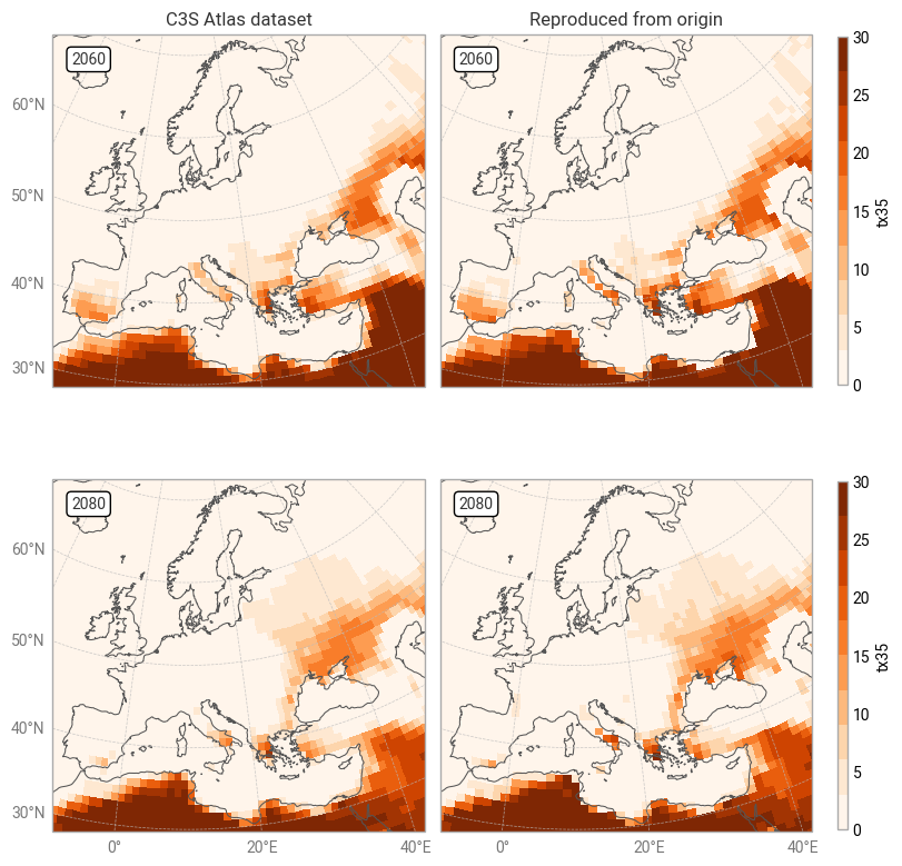
Fig. 7.1.2 Comparison between C3S Atlas dataset and reproduction for one indicator (tx35) in one month, across Europe, on the native grid of each dataset.

Show code cell source

Hide code cell source

geospatial_comparison(indicators_c3s_atlas, indicators_cmip6, indicator, month, domain="global",
                      glue_label="derived_multi-origin-c3s-atlas_consistency_q01_fig-geo-global")

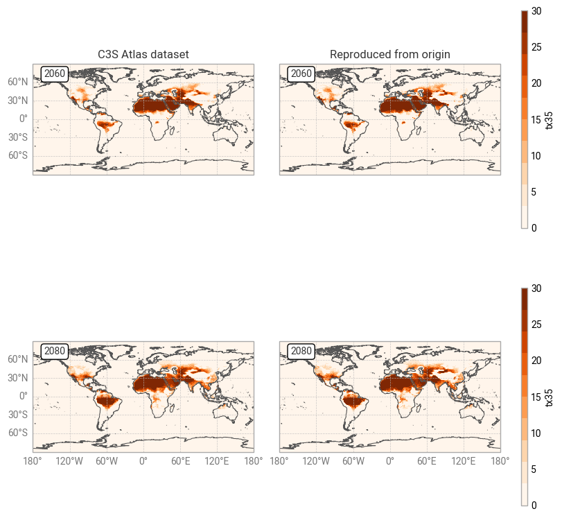
Fig. 7.1.3 Comparison between C3S Atlas dataset and reproduction for one indicator (tx35) in one month, across the globe, on the native grid of each dataset.

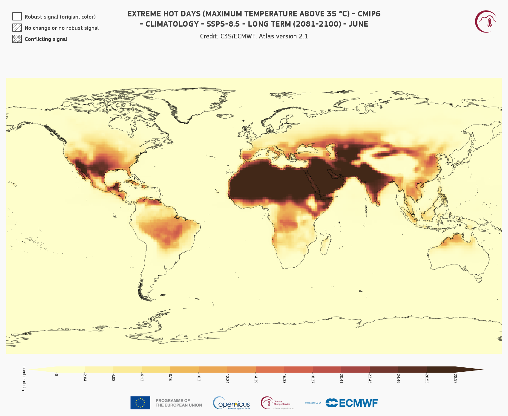
Fig. 7.1.4 C3S Atlas application view of tx35 indicator in June, averaged 2081–2100 in the SSP5-8.5 scenario, for comparison with Figure 7.1.3.

Show code cell source

Hide code cell source

# Histogram
fig_hist = histogram_comparison_by_year(indicators_c3s_atlas, indicators_cmip6, indicator,
                                        glue_label="derived_multi-origin-c3s-atlas_consistency_q01_fig-hist-native")

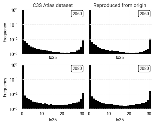
Fig. 7.1.5 Comparison between overall distributions of indicator (tx35) values in the C3S Atlas dataset and its reproduction, across all spatial and temporal dimensions, on the native grid of each dataset.

Reproducibility: Comparison on C3S Atlas grid

After regridding to the C3S Atlas grid, the indicator values reproduced from the origin dataset can be compared point-by-point to the values retrieved from the C3S Atlas dataset. We first examine some metrics that describe the difference Δ between corresponding pixels:

Show code cell source

Hide code cell source

display_difference_stats(indicators_c3s_atlas, indicators_cmip6_regridded, indicator)

C3S Atlas – Reproduced

	Mean Δ	Median Δ	Median |Δ|	% where |Δ| ≥ ε	Median |Δ| [%]	Pearson r
2060	-0.00077	0.00000	0.00000	0.07665	0.00000	0.99998
2080	-0.00095	0.00000	0.00000	0.09388	0.00000	0.99998

It is clear that the two datasets are extremely close: the median difference and median absolute difference are both 0 and fewer than 0.1% of pixel pairs show a non-zero difference (defined here as |Δ| ≥ ε with ε = 10^–5 to avoid floating-point errors). We can immediately conclude that the C3S Atlas dataset is highly reproducible from its origins using the provided workflow.

This conclusion is strengthened by examining the distributions of indicator values and their point-by-point differences (Figure 7.1.6). The vast majority of pixel pairs have a difference of 0, with very few ±1 and even fewer ±2 (note the logarithmic y-axis).

However, this raises an obvious question: why are there any differences at all? The geospatial distribution of differences (Figure 7.1.7) does not appear to correlate with any patterns in the indicator values themselves nor in geography. Since the differences are very small and seemingly random, a potential explanation is that they simply result from small changes in the origin dataset and/or the C3S Atlas workflow software between the production of the C3S Atlas dataset and the present day. Testing this hypothesis would require an extremely detailed analysis of all steps in the workflow, which is outside the scope of this assessment.

Setting this question affecting <0.1% of pixels aside, we can confidently conclude from the metrics and figures that the C3S Atlas dataset is highly reproducible from its origins using the provided workflow, at least for the tx35 indicator and CMIP6 dataset.

Show code cell source

Hide code cell source

# Histogram
fig_hist = histogram_comparison_by_year_with_difference(indicators_c3s_atlas, indicators_cmip6_regridded, indicator,
                                                        glue_label="derived_multi-origin-c3s-atlas_consistency_q01_fig-hist-c3s-atlas")

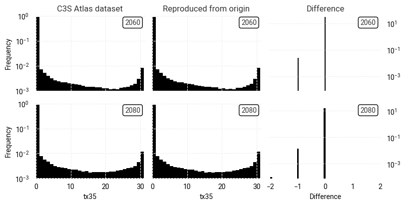
Fig. 7.1.6 Comparison between overall distributions of indicator (tx35) values in the C3S Atlas dataset and its reproduction on the C3S Atlas grid, across all spatial and temporal dimensions, including the per-pixel difference.

Show code cell source

Hide code cell source

# Create plot with function defined at the start
geospatial_comparison_with_difference(indicators_c3s_atlas, indicators_cmip6_regridded, indicator, month, domain=domain,
                                      glue_label="derived_multi-origin-c3s-atlas_consistency_q01_fig-geocomp-regional")

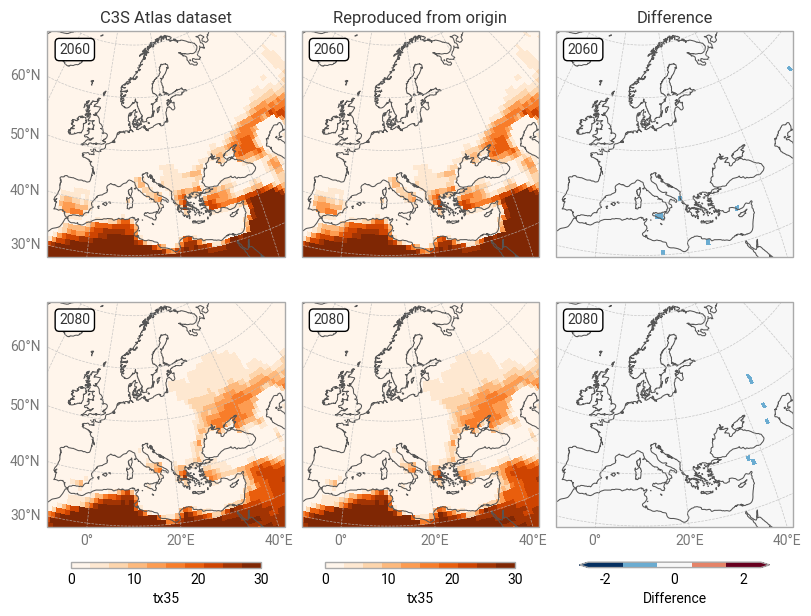
Fig. 7.1.7 Comparison between C3S Atlas dataset and reproduction for one indicator (tx35) in one month, across Europe, on the C3S Atlas dataset grid, including the per-pixel difference.

ℹ️ If you want to know more

Key resources

The CDS catalogue entries for the data used were:

• Gridded dataset underpinning the Copernicus Interactive Climate Atlas: multi-origin-c3s-atlas

  • Consistency between the C3S Atlas dataset and its origins: Case study

  • Consistency between the C3S Atlas dataset and its origins: Multiple indicators

  • Consistency between the C3S Atlas dataset and its origins: Multiple origin datasets

• CMIP6 climate projections: projections-cmip6

  • Quality assessments for CMIP6

Code libraries used:

• earthkit

  • earthkit-data

  • earthkit-plots

• User-tools for the C3S Atlas

• xclim climate indicator tools

More about the Copernicus Interactive Climate Atlas and its IPCC predecessor:

• Copernicus Interactive Climate Atlas application

• Gridded data underpinning the Copernicus Interactive Climate Atlas: Description of the datasets and variables

• The Copernicus Interactive Climate Atlas: a tool to explore regional climate change

• Copernicus Interactive Climate Atlas: a new tool to visualise climate variability and change

• Implementation of FAIR principles in the IPCC: the WGI AR6 Atlas repository

• Climate Change 2021 – The Physical Science Basis: Atlas

References

[Gutiérrez+24] J. M. Gutiérrez et al., ‘The Copernicus Interactive Climate Atlas: a tool to explore regional climate change’, ECMWF Newsletter, vol. 181, pp. 38–45, Oct. 2024, doi: 10.21957/ah52ufc369.

[C3S Atlas dataset] Copernicus Climate Change Service, ‘Gridded dataset underpinning the Copernicus Interactive Climate Atlas’. Copernicus Climate Change Service (C3S) Climate Data Store (CDS), Jun. 17, 2024. doi: 10.24381/cds.h35hb680.

[CMIP6 dataset] Copernicus Climate Change Service, ‘CMIP6 climate projections’. Copernicus Climate Change Service (C3S) Climate Data Store (CDS), Mar. 23, 2021. doi: 10.24381/cds.c866074c.

[Burggraaff+20] O. Burggraaff, ‘Biases from incorrect reflectance convolution’, Optics Express, vol. 28, no. 9, pp. 13801–13816, Apr. 2020, doi: 10.1364/OE.391470.