1. Reproducibility of the C3S Atlas Dataset

This initial chapter provides several notebooks designed to reproduce the calculation of gridded data (variables and indices, see Table 3) included in the C3S Atlas Dataset. These notebooks promote reusability and enable rapid development of customized products tailored to specific applications. Note, however, that the notebook examples cover only specific regions and subsets and cannot be used directly to replicate the entire dataset, as it requires an optimized workflow executed on HPC infrastructure.

Figure 1 provides a schematic representation of the data production workflow, emphasizing the following processing steps:

• Download climate data from the C3S-CDS using the CDS API.

• Download the reference datasets (only for bias adjusted indices).

• Perform data homogenization to ensure the same calendar time, coordinate names, variable units, dimension order, among other things.

• Interpolate both the projections and the reference dataset to a regular-common grid using conservative remapping (only for bias adjusted indices).

• Calculate the index.

• Perform temporal aggregation.

• Interpolate to a regular-common grid using conservative remapping (not necessary for bias adjusted indices).

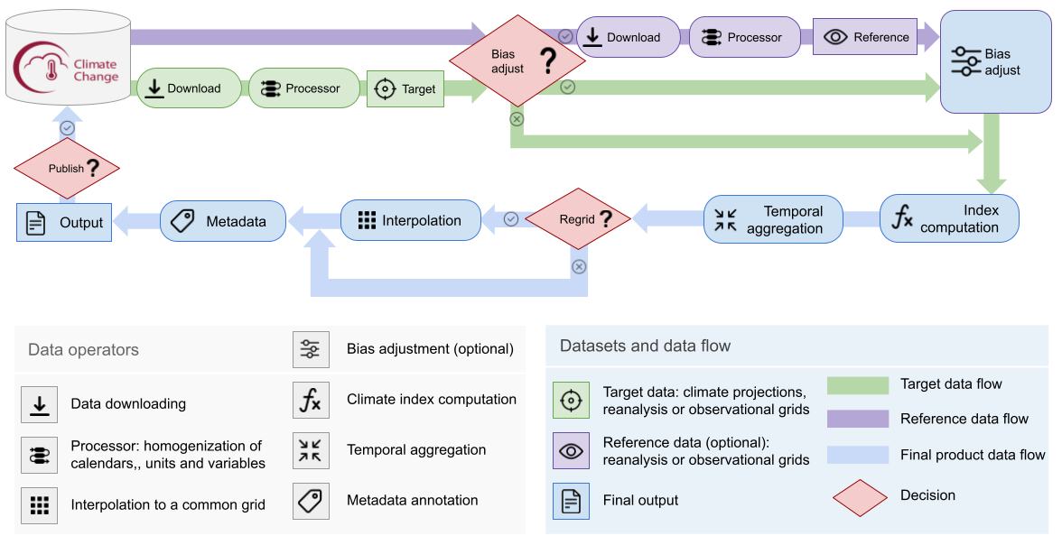
Figure 1. Schematic diagram of the C3S Atlas data production workflow.

Table 1 lists the notebooks included in this chapter, describing the application of the workflow in cases with different complexity (e.g. with and without bias adjustment).

Directory	Contents
tx35.ipynb	Jupyter Notebook for calculating the “number of days with maximum temperature over 35°C” (TX35) index using xclim library.
tx35bals.ipynb	Jupyter Notebook for calculating “number of days with bias-adjusted maximum temperature over 35°C” (TX35bals) index using xclim and ibicus libraries.
cd.ipynb	Jupyter Notebook for calculating the “Cooling Degree-Days” (CD) index using in-house index funtions.
cddbaisimip.ipynb	Jupyter Notebook for calculating the bias-adjusted (ISIMIP) precipitation “Consecutive Dry Days (CDD)” index with bias-adjusted (ISIMIP) precipitation using xclim and ibicus funtions.

Table 1. Notebooks included as example to reproduce the C3S Atlas data production workflow.

Open Python libraries

Table 2 displays the list of Python libraries used for the implementation of the workflow for index calculation.

Library	Description
xarray	Python library for managing labelled multi-dimensional arrays.
xclim	xclim is a library for climate index calculation built using xarray and can seamlessly benefit from the parallelization handling provided by dask.
ibicus	Bias adjustment library for climate model data adjustment using observational references.
xESMF	Regridding library for geospatial data.
cdsapi	The Climate Data Store (CDS) Application Program Interface (API) is a service providing programmatic access to CDS data

Table 2. List of Python libraries used in the C3S Atlas workflow.

List of indices

Table 3 shows the climate variables and indices included in the C3S Atlas dataset (v2).

Code	Name Data	Unit Data	Description data	Implementation
t	Monthly mean of daily mean temperature	degC	Monthly mean of daily mean near-surface (2-metre) air temperature	t.resample(time=’MS’).mean()
tn	Monthly mean of daily minimum temperature	degC	Monthly mean of daily minimum near-surface (2-metre) air temperature	tn.resample(time=’MS’).mean()
tx	Monthly mean of daily maximum temperature	degC	Monthly mean of daily maximum near-surface (2-metre) air temperature	tx.resample(time=’MS’).mean()
tnn	Monthly minimum of daily minimum temperature	degC	Monthly minimum of daily minimum near-surface (2-metre) air temperature	tn.resample(time=’MS’).min()
txx	Monthly maximum of daily maximum temperature	degC	Monthly maximum of daily maximum near-surface (2-metre) air temperature	tx.resample(time=’MS’).max()
tx35	Monthly count of days with maximum temperature above 35 degC	1	Monthly count of days with maximum near-surface (2-metre) air temperature above 35 degC	xclim.indices.tx_days_above(tx, thresh=’35.0 degC’, freq=’MS’, op=’>’)
tx40	Monthly count of days with maximum temperature above 40 degC	1	Monthly count of days with maximum near-surface (2-metre) air temperature above 40 degC	xclim.indices.tx_days_above(tx, thresh=’40.0 degC’, freq=’MS’, op=’>’)
tr	Monthly count of tropical nights (days with minimum temperature above 20 degC)	1	Monthly count of days with minimum near-surface (2-metre) air temperature above 20 degC	xclim.indicators.atmos.tropical_nights(tasmin=tn, thresh=’20.0 degC’, freq=’MS’, op=’>’)
dtr	Monthly mean of daily temperature range	degC	Monthly mean of daily near-surface (2-metre) air temperature range	xclim.indices.daily_temperature_range(tn, tx, freq=’MS’, op=’mean’)
fd	Monthly count of frost days	1	Monthly count of days with minimum near-surface (2-metre) air temperature below 0 degC	xclim.indicators.atmos.frost_days(tn, thresh=’0 degC’, freq=’MS’)
hd	Annual heating degree-days	degC day	Annual energy consumption to heat the deficit of temperature below 15.5 degC	c3s_atlas.lib.indexes.hd(t, tx, tn, freq=’YS’, thresh=15.5)
cd	Annual cooling degree-days	degC day	Annual energy consumption to cool the excess of temperature above 22 degC	c3s_atlas.lib.indexes.cd(t, tx, tn, freq=’YS’, thresh=22)
r	Monthly mean of daily accumulated precipitation	mm	Monthly mean of daily accumulated precipitation of liquid water equivalent from all phases	r.resample(time=’MS’).mean()
r01	Monthly count of days with daily accumulated precipitation above 1 mm	1	Monthly count of days with daily accumulated precipitation of liquid water equivalent from all phases above 1 mm	xclim.indices.days_over_precip_thresh(r, 0, thresh=’1 mm/day’, freq=’MS’, bootstrap=False, op=’>’)
sdii	Monthly mean of daily accumulated precipitation on wet days (above 1 mm)	mm	Monthly average of daily precipitation amount of liquid water equivalent from all phases on days with precipitation amount above or equal to 1 mm	xclim.indicators.atmos.daily_pr_intensity(r=r, thresh=’1 mm/day’, freq=’MS’, op=’>=’)
r10	Monthly count of days with daily accumulated precipitation above 10 mm	1	Monthly count of days with daily accumulated precipitation of liquid water equivalent from all phases above 10 mm	xclim.indices.days_over_precip_thresh(r, 0, thresh=’10 mm/day’, freq=’MS’, bootstrap=False, op=’>’)
r20	Monthly count of days with daily accumulated precipitation above 20 mm	1	Monthly count of days with daily accumulated precipitation of liquid water equivalent from all phases above 20 mm	xclim.indices.days_over_precip_thresh(r, 0, thresh=’20 mm/day’, freq=’MS’, bootstrap=False, op=’>’)
rx1day	Monthly maximum of 1-day accumulated precipitation	mm	Monthly maximum of 1-day accumulated precipitation of liquid water equivalent from all phases	xclim.indicators.atmos.max_n_day_precipitation_amount(r, window=1, freq=’MS’)
rx5day	Monthly maximum of 5-day accumulated precipitation	mm	Monthly maximum of 5-day accumulated precipitation of liquid water equivalent from all phases	xclim.indicators.atmos.max_n_day_precipitation_amount(r, window=5, freq=’MS’)
cdd	Annual maximum consecutive dry days (below 1 mm)	day	Annual maximum of consecutive days when daily accumulated precipitation amount is below 1 mm	xclim.indices.maximum_consecutive_dry_days(r, thresh=’1 mm/day’, freq=’YS’, resample_before_rl=True)
spi6	Monthly Standardised Precipitation Index (SPI) for 6 months cumulation period	1	Monthly index that compares accumulated precipitation for 6 months with the long-term precipitation distribution for the same location and accumulation period, as the number of standard deviations from the mean. The reference period corresponds to 1971-2010 for observations, reanalysis, and historical projections, and to 1971-2100 for the future scenario projections	xclim.indices.standardized_precipitation_index(r, r_cal, freq=”MS”, window =6, dist=”gamma”, method=”ML”)
spei6	Monthly Standardised Precipitation-Evapotranspiration Index (SPEI) for 6 months cumulation period	1	Monthly index that compares accumulated precipitation minus potential evapotranspiration (Hargreaves 1985, 1994 method) for 6 months with the long-term distribution for the same location and accumulation period, as the number of standard deviations from the mean. The reference period corresponds to 1971-2010 for observations, reanalysis, and historical projections, and to 1971-2100 for the future scenario projections	xclim.indices.standardized_precipitation_evapotranspiration_index(wb, wb_cal, freq=”MS”, window=6, dist=”fisk”, method=”ML”, offset = abs(np.min(wb)))
pet	Monthly mean of daily accumulated potential evapotranspiration	mm	Potential evapotranspiration (Hargreaves 1985, 1994) is the rate at which evapotranspiration would occur under ambient conditions from a uniformly vegetated area when the water supply is not limiting	xclim.indices.potential_evapotranspiration(tn, tx, method=’HG85’)
huss	Monthly mean near surface specific humidity	gr kg-1	Monthly amount of moisture in the air near the surface (2-metre) divided by amount of air plus moisture	huss.resample(time=’MS’).mean()
evspsbl	Monthly mean of daily accumulated evaporation (including sublimation and transpiration)	mm	Monthly mean of daily amount of water in the atmosphere due to conversion of both liquid and solid phases to vapor (from underlying surface and vegetation)	evspsbl.resample(time=’MS’).mean()
mrsos	Monthly mean of daily accumulated soil moisture in upper soil portion	kg m-2	Monthly soil shallow moisture content, as the vertical sum per unit area of water in all phases contained in the upper soil portion to a depth of 7 to 10 cm (depending on the dataset)	mrsos.resample(time=’MS’).mean()
mrro	Monthly mean of daily accumulated runoff	mm	Monthly mean of daily amount per unit area of surface and subsurface liquid water which drains from land	mrro.resample(time=’MS’).mean()
prsn	Monthly mean of daily accumulated snowfall precipitation	mm	Monthly mean of daily accumulated liquid water equivalent thickness snowfall	prsn.resample(time=’MS’).mean()
siconc	Monthly mean of sea-ice area percentage	percent	Monthly mean fraction (%) of sea grid cell area covered by ice	siconc.resample(time=’MS’).mean()
sfcwind	Monthly mean of daily mean wind speed	m s-1	Monthly mean of daily mean near-surface (10-metre) wind speed	sfcwind.resample(time=’MS’).mean()
clt	Monthly mean cloud cover area percentage	%	Monthly mean fraction (%) of the sky covered by clouds	clt.resample(time=’MS’).mean()
rsds	Monthly mean of surface solar radiation downwards	W m-2	Monthly mean of incident solar (shortwave) radiation that reaches a horizontal plane at the surface	rsds.resample(time=’MS’).mean()
rlds	Monthly mean of surface thermal radiation downwards	W m-2	Monthly incident thermal (longwave) radiation at the surface (during cloudless and overcast conditions)	rlds.resample(time=’MS’).mean()
sst	Monthly mean of sea surface temperature	degC	Monthly mean temperature of sea water near the surface	sst.resample(time=’MS’).mean()
psl	Monthly average of mean sea level pressure	hPa	Monthly average air pressure at mean sea level	psl.resample(time=’MS’).mean()

Table 3. Description of the climate variables and indices included in the second version of the C3S Atlas. The first four columns indicate the code, name, units, and description of the indices. The last column includes the Python command used to compute the C3S Atlas indices from daily data, either using xarray, xclim or in-house. Input variables used to compute each index are defined with its code name (e.g. t for daily mean air temperature) functions.

Bias corrected indices

For threshold-dependent indices the C3S Atlas includes both raw and bias-adjusted information, using two alternative methods: the simple LinearScaling (Douglas Maraun 2016) and more advanced trend preserving method ISIMIP (Lange 2019).

Ibiscu Method	Function	Parameters	Description
LinearScaling	LinearScaling (daily temperature, t)	“running_window_mode”: True, “running_window_length”: 30, “running_window_step_length”: 30	Linear scaling method based on Douglas Maraun 2016. Reference period used for BA: 1980-2005 (CMIP5/6 using WFDE5) and 1970-2005 (CORDEX-EUR-11 using E-OBS and CORDEX-CORE using ERA5-Land)
ISIMIP	ISIMIP (daily temperature, t)	“running_window_mode”: False	ISIMIP trend preserving method based on Lange 2021. Reference period used for BA: 1980-2005 (CMIP5/6 using WFDE5) and 1970-2005 (CORDEX-EUR-11 using E-OBS and CORDEX-CORE using ERA5-Land)
ISIMIP	ISIMIP (daily precipitation; r)	“lower_bound”: 0, “lower_threshold”: 0.1, “upper_bound”: np.inf, “upper_threshold”: np.inf, “distribution”: scipy.stats.gamma, “trend_preservation_method”: “mixed”, “running_window_mode”: False

Table 4. Specific functions and parameters of the Python Ibicus package used in the C3S Atlas for bias-adjusted variables.