

1.4. Consecutive Dry Days with bias adjusted precipitation#
This Jupyter Notebook calculates the variable cdd (Annual maximum consecutive dry days -below 1 mm-) with bias adjustment (ba) using the ISIMIP trend preserving method based on (Lange 2019) (cddbaismip) for the CMIP6-CMCC_ESM2 model. WFDE5 is used as reference dataset for the “ba”.
For quick demonstration purposes, a small region in the north of Spain is selected.
First, the raw CMIP6 model and the reference dataset (WFDE5) needed for bias adjustment are downloaded from the CDS. Then, the CMIP6 model is bias-adjusted, and the results are compared with the “Gridded dataset underpinning the Copernicus Interactive Climate Atlas”, which is also downloaded from the CDS.
Please be advised that downloading the required data for this script may take several minutes.
1.4.1. Load Python packages and clone and install the c3s-atlas GitHub repository from the ecmwf-projects#
Clone (git clone) the c3s-atlas repository and install them (pip install -e .).
Further details on how to clone and install the repository are available in the requirements section
import cdsapi
import os
from pathlib import Path
import xarray as xr
import xclim
import numpy as np
import pandas as pd
import matplotlib.pyplot as plt
import cartopy.crs as ccrs
import glob
from ibicus.debias import ISIMIP
import scipy
import matplotlib.pyplot as plt

from c3s_atlas.utils import (
    extract_zip_and_delete,
    get_ds_to_fill,
    plot_month
)
from c3s_atlas.fixers import (
    apply_fixers
)
import c3s_atlas.interpolation as xesmfCICA
1.4.2. Download climate data with the CDS API#
To reduce data size and download time, a geographical subset focusing on a specific area within the European region (Spain) is selected.
Catalogues:
WFDE5: Note that for WFDE5, the subsetting function is not available on the CDS side. To limit the saved data, the entire global dataset is downloaded and then cropped to the Spanish area.
cdsapi_url= "https://cds.climate.copernicus.eu/api"
cdsapi_key= ""
c = cdsapi.Client(url=cdsapi_url, key=cdsapi_key)
⚠️ Warning: Exposed API Credentials
For security reasons, it is not recommended to hardcode your Copernicus Climate Data Store (CDS) API credentials — such as
cdsapi_urlandcdsapi_key— directly in notebooks.Instead, it is best to store them securely in a
.cdsapircfile located in your home directory.📄 More info: CDS API - How to use the API
# define some global attributes for the CDS-API
CMIP6_years = {
    "historical": [str(n) for n in np.arange(1980, 2006)],
    "ssp5_8_5": [str(n) for n in np.arange(2015, 2100)]
}
# variables
variables = {
    'pr': 'precipitation',
}
# directory to download the files
file_dest_CMIP6 = Path('./data/CMIP6')
file_dest_WFDE5 = Path('./data/WFDE5')
months = [
    '01', '02', '03',
    '04', '05', '06',
    '07', '08', '09',
    '10', '11', '12'
]

days = [
    '01', '02', '03',
    '04', '05', '06',
    '07', '08', '09',
    '10', '11', '12',
    '13', '14', '15',
    '16', '17', '18',
    '19', '20', '21',
    '22', '23', '24',
    '25', '26', '27',
    '28', '29', '30', '31'
]
Download CMIP6 data#
Period 2015-2100 for the ssp5_8_5 scenario
Period 1980-2006 for the historical scenario.
os.makedirs(file_dest_CMIP6, exist_ok=True)

for experiment in CMIP6_years.keys():
    for year in CMIP6_years[experiment]:
        for var in variables.keys():
            path_zip = file_dest_CMIP6 / f"CMIP6_{var}_{experiment}_{year}.zip"
            c.retrieve(
                'projections-cmip6',
                {
                    'temporal_resolution': 'daily',
                    'variable': variables[var],
                    'experiment': experiment,
                    'model': 'cmcc_esm2',
                    'year': [year],
                    'month': months,
                    'day': days,
                    'area':[45.5, 5.5, 34, -11.5], # crop area for Spain
                }).download(path_zip)
            # Extract zip file into the specified directory and remove zip
            extract_zip_and_delete(path_zip)
Download WFDE5 data#
Period 1980-2006
# variables
variables = {
    'pr': 'rainfall_flux',
}
os.makedirs(file_dest_WFDE5, exist_ok=True)

for year in CMIP6_years['historical']:
    for month in months:
        for var in variables.keys():
            path_zip = file_dest_WFDE5 / f"WFDE5_{var}_{year}_{month}_globe.zip"
            c.retrieve(
                'derived-near-surface-meteorological-variables',
                {
                    'version': '2_1',
                    'month': month,
                    'reference_dataset': 'cru',
                    'variable': variables[var],
                    'year': year,
                }).download(path_zip)
            # Extract zip file into the specified directory and remove zip
            extract_zip_and_delete(path_zip)
            # Crop area an save
            ds = xr.open_dataset(path_zip.with_suffix(".nc"))
            ds = ds.sel(lat = slice(34, 45.5), lon = slice(-11.5 , 5.5))
            file = file_dest_WFDE5 / f"WFDE5_{var}_{year}_{month}.nc"
            ds.to_netcdf(file)
            os.remove(path_zip.with_suffix(".nc"))
1.4.3. Load files with xarray#
# load CMIP6 files
ds_CMIP6_hist = xr.open_mfdataset(
    np.sort(glob.glob(str(file_dest_CMIP6 / "*pr_historical*.nc"))),
    concat_dim='time', combine='nested'
)

ds_CMIP6_ssp585 = xr.open_mfdataset(
    np.sort(glob.glob(str(file_dest_CMIP6 / "*pr_ssp5_8_5*.nc"))),
    concat_dim='time', combine='nested'
)
# load WFDE5 files
ds_WFDE5_hist = xr.open_mfdataset(
    np.sort(glob.glob(str(file_dest_WFDE5 / "*WFDE5_pr*.nc"))),
    concat_dim='time', combine='nested'
)
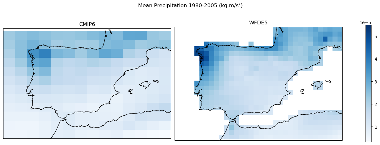
Visualize downloaded datasets#
fig, axes = plt.subplots(1, 2, figsize=(12, 5), constrained_layout=True,
                        subplot_kw={'projection': ccrs.PlateCarree()}, sharey=True)

data_cmip6 = ds_CMIP6_hist['pr'].sel(
    time=slice('1980-01-01', '2005-12-31')).mean(dim = 'time')
data_wfde5 = ds_WFDE5_hist['Rainf'].sel(
    time=slice('1980-01-01', '2005-12-31')).mean(dim = 'time')

vmin = min(data_cmip6.min(), data_wfde5.min()).values
vmax = max(data_cmip6.max(), data_wfde5.max()).values

data_cmip6.plot(ax=axes[0], cmap="Blues", vmin=vmin, vmax=vmax, add_colorbar=False)
axes[0].set_title("CMIP6")
axes[0].coastlines()

data_wfde5.plot(ax=axes[1], cmap="Blues", vmin=vmin, vmax=vmax, add_colorbar=False)
axes[1].set_title("WFDE5")
axes[1].coastlines()

cbar = fig.colorbar(plt.cm.ScalarMappable(cmap="Blues", norm=plt.Normalize(vmin=vmin, vmax=vmax)),
                    ax=axes, orientation='vertical', shrink=0.8)
fig.suptitle("Mean Precipitation 1980-2005 (kg.m/s²)")
Text(0.5, 0.98, 'Mean Precipitation 1980-2005 (kg.m/s²)')
1.4.4. Homogenization#
Once the data is downloaded from the CDS it undergoes a process of homogenization:
The metadata of the spatial coordinates is homogenised to use standard names, in particular [lon, lat].
Fix any non-standard calendars used in the data. This typically involves converting the calendars to the CF standard calendar (Mixed Gregorian/Julian) commonly used in climate data.
Convert the units of the data to a common format (e.g. Celsius for temperature). This prevents us from working with the same variables in different units, for example.
Convert the longitude values from the [0, 360] format to the [-180, 180] one. This is done to ensure that the longitude variable is common between the different datasets.
Aggregated to the required temporal resolution. For example, hourly datasets (such as ERA5, ERA5-Land, WFDE5, etc.) will be resampled to daily resolution. This involves using a temporal aggregation method, such as taking the maximum or minimum value for a given variable. As part of this last step, some variable transformations are necessarily applied. For instance, fluxes variables in ERA5 are accumulated, and therefore, the last hour of the day represent daily accumulations. To mention another case, the surface wind is computed as a combination of both the u- and v-components.
project_id = "cmip6"
variable = 'pr'
var_mapping = {
            "dataset_variable": {"pr": "pr"},
            "aggregation": {"pr": "mean"},
        }
ds_CMIP6_hist = apply_fixers(ds_CMIP6_hist, variable, project_id, var_mapping)
ds_CMIP6_ssp585 = apply_fixers(ds_CMIP6_ssp585, variable, project_id, var_mapping)
2025-05-20 11:27:24,091 — Homogenization-fixers — INFO — Dataset has already the correct names for its coordinates
2025-05-20 11:27:24,157 — Homogenization-fixers — INFO — Fixing calendar for <xarray.Dataset> Size: 11MB
Dimensions:    (time: 9490, bnds: 2, lat: 12, lon: 14)
Coordinates:
  * time       (time) object 76kB 1980-01-01 12:00:00 ... 2005-12-31 12:00:00
  * lat        (lat) float64 96B 34.4 35.34 36.28 37.23 ... 42.88 43.82 44.76
  * lon        (lon) float64 112B -11.25 -10.0 -8.75 -7.5 ... 1.25 2.5 3.75 5.0
Dimensions without coordinates: bnds
Data variables:
    time_bnds  (time, bnds) object 152kB dask.array<chunksize=(1, 2), meta=np.ndarray>
    lat_bnds   (time, lat, bnds) float64 2MB dask.array<chunksize=(365, 12, 2), meta=np.ndarray>
    lon_bnds   (time, lon, bnds) float64 2MB dask.array<chunksize=(365, 14, 2), meta=np.ndarray>
    pr         (time, lat, lon) float32 6MB dask.array<chunksize=(1, 12, 14), meta=np.ndarray>
Attributes: (12/48)
    Conventions:            CF-1.7 CMIP-6.2
    activity_id:            CMIP
    branch_method:          standard
    branch_time_in_child:   0.0
    branch_time_in_parent:  0.0
    comment:                none
    ...                     ...
    title:                  CMCC-ESM2 output prepared for CMIP6
    variable_id:            pr
    variant_label:          r1i1p1f1
    license:                CMIP6 model data produced by CMCC is licensed und...
    cmor_version:           3.6.0
    tracking_id:            hdl:21.14100/9c81777c-32b6-4da9-bb1d-5f82f76f0354
2025-05-20 11:27:24,511 — UNITS_TRANSFORM — INFO — The dataset pr units are not in the correct magnitude. A conversion from kg m-2 s-1 to mm will be performed.
2025-05-20 11:27:24,736 — Homogenization-fixers — INFO — The dataset is in daily or monthly resolution, we don't need to resample it from hourly frequency
2025-05-20 11:27:24,738 — Homogenization-fixers — INFO — Dataset has already the correct names for its coordinates
2025-05-20 11:27:24,874 — Homogenization-fixers — INFO — Fixing calendar for <xarray.Dataset> Size: 35MB
Dimensions:    (time: 31025, bnds: 2, lat: 12, lon: 14)
Coordinates:
  * time       (time) object 248kB 2015-01-01 12:00:00 ... 2099-12-31 12:00:00
  * lat        (lat) float64 96B 34.4 35.34 36.28 37.23 ... 42.88 43.82 44.76
  * lon        (lon) float64 112B -11.25 -10.0 -8.75 -7.5 ... 1.25 2.5 3.75 5.0
Dimensions without coordinates: bnds
Data variables:
    time_bnds  (time, bnds) object 496kB dask.array<chunksize=(1, 2), meta=np.ndarray>
    lat_bnds   (time, lat, bnds) float64 6MB dask.array<chunksize=(365, 12, 2), meta=np.ndarray>
    lon_bnds   (time, lon, bnds) float64 7MB dask.array<chunksize=(365, 14, 2), meta=np.ndarray>
    pr         (time, lat, lon) float32 21MB dask.array<chunksize=(1, 12, 14), meta=np.ndarray>
Attributes: (12/48)
    Conventions:            CF-1.7 CMIP-6.2
    activity_id:            ScenarioMIP
    branch_method:          standard
    branch_time_in_child:   60225.0
    branch_time_in_parent:  60225.0
    comment:                none
    ...                     ...
    title:                  CMCC-ESM2 output prepared for CMIP6
    variable_id:            pr
    variant_label:          r1i1p1f1
    license:                CMIP6 model data produced by CMCC is licensed und...
    cmor_version:           3.6.0
    tracking_id:            hdl:21.14100/0c6732f7-2cdd-4296-99a0-7952b7ca911e
2025-05-20 11:27:25,688 — UNITS_TRANSFORM — INFO — The dataset pr units are not in the correct magnitude. A conversion from kg m-2 s-1 to mm will be performed.
2025-05-20 11:27:25,883 — Homogenization-fixers — INFO — The dataset is in daily or monthly resolution, we don't need to resample it from hourly frequency
project_id = "WFDE5"
variable = 'pr'
var_mapping = {
            "dataset_variable": {"pr": "Rainf"},
            "aggregation": {"pr": "mean"},
        }
ds_WFDE5_hist = apply_fixers(ds_WFDE5_hist, variable, project_id, var_mapping)
2025-05-20 11:27:25,890 — Homogenization-fixers — INFO — Dataset has already the correct names for its coordinates
2025-05-20 11:27:25,955 — Homogenization-fixers — INFO — Fixing calendar for <xarray.Dataset> Size: 715MB
Dimensions:  (time: 227928, lat: 23, lon: 34)
Coordinates:
  * lat      (lat) float64 184B 34.25 34.75 35.25 35.75 ... 44.25 44.75 45.25
  * lon      (lon) float64 272B -11.25 -10.75 -10.25 -9.75 ... 4.25 4.75 5.25
  * time     (time) datetime64[ns] 2MB 1980-01-01 ... 2005-12-31T23:00:00
Data variables:
    Rainf    (time, lat, lon) float32 713MB dask.array<chunksize=(744, 23, 34), meta=np.ndarray>
Attributes:
    title:        WATCH Forcing Data methodology applied to ERA5 data
    institution:  Copernicus Climate Change Service
    contact:      http://copernicus-support.ecmwf.int
    comment:      Methodology implementation for ERA5 and dataset production ...
    Conventions:  CF-1.7
    summary:      ERA5 data regridded to half degree regular lat-lon; Genuine...
    reference:    Cucchi et al., 2020, Earth Syst. Sci. Data, 12(3), 2097–212...
    licence:      The dataset is distributed under the Licence to Use Coperni...
2025-05-20 11:27:25,985 — UNITS_TRANSFORM — INFO — The dataset pr units are not in the correct magnitude. A conversion from kg m-2 s-1 to mm will be performed.
2025-05-20 11:27:26,013 — Homogenization-fixers — INFO — The dataset is in hourly resolution, we need to resample it to daily resolution
2025-05-20 11:27:49,932 — Homogenization-fixers — INFO — Dataset resampled to daily resolution
1.4.5. Interpolation to a common and regular grid using xESMF#
A wrapper for the xESMF Python package was developed within the framework of the C3S Atlas project to extend its functionalities to all datasets (regular, curvilinear, etc.)
# interpolate data
int_attr = {'interpolation_method' : 'conservative_normed',
            'lats' : np.arange(34.5, 46.5, 1),
            'lons' : np.arange(-11.5, 6.5, 1),
            'var_name' : 'pr'
}
INTER = xesmfCICA.Interpolator(int_attr)
ds_CMIP6_hist_i = INTER(ds_CMIP6_hist)
ds_CMIP6_ssp585_i = INTER(ds_CMIP6_ssp585)
ds_WFDE5_hist_i = INTER(ds_WFDE5_hist)
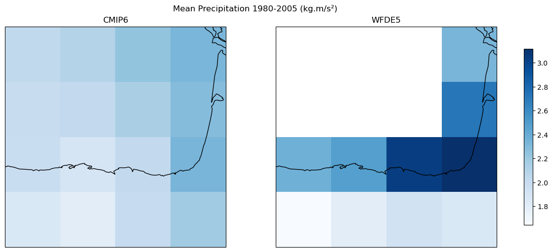
Crop small area in the north of Spain#
ds_CMIP6_hist_i = ds_CMIP6_hist_i.sel(lon = slice(-5, -1), lat = slice(42, 46))
ds_CMIP6_ssp585_i = ds_CMIP6_ssp585_i.sel(lon = slice(-5, -1), lat = slice(42, 46))
ds_WFDE5_hist_i = ds_WFDE5_hist_i.sel(lon = slice(-5, -1), lat = slice(42, 46))
fig, axes = plt.subplots(1, 2, figsize=(12, 5), constrained_layout=True,
                        subplot_kw={'projection': ccrs.PlateCarree()}, sharey=True)

data_cmip6 = ds_CMIP6_hist_i['pr'].sel(
    time=slice('1980-01-01', '2005-12-31')).mean(dim = 'time')
data_wfde5 = ds_WFDE5_hist_i['pr'].sel(
    time=slice('1980-01-01', '2005-12-31')).mean(dim = 'time')

vmin = min(data_cmip6.min(), data_wfde5.min()).values
vmax = max(data_cmip6.max(), data_wfde5.max()).values

data_cmip6.plot(ax=axes[0], cmap="Blues", vmin=vmin, vmax=vmax, add_colorbar=False)
axes[0].set_title("CMIP6")
axes[0].coastlines()

data_wfde5.plot(ax=axes[1], cmap="Blues", vmin=vmin, vmax=vmax, add_colorbar=False)
axes[1].set_title("WFDE5")
axes[1].coastlines()

cbar = fig.colorbar(plt.cm.ScalarMappable(cmap="Blues", norm=plt.Normalize(vmin=vmin, vmax=vmax)), ax=axes, orientation='vertical', shrink=0.8)
fig.suptitle("Mean Precipitation 1980-2005 (kg.m/s²)")
Text(0.5, 0.98, 'Mean Precipitation 1980-2005 (kg.m/s²)')
1.4.6. Bias adjustment using ibicus#
Two methods of ba are applied in the C3S Atlas: the LinearScaling (Douglas Maraun 2016) and the ISIMIP (Lange 2019). Here, for simplicity, we applied the linear scaling one.
args = {
    "lower_bound": 0,
    "lower_threshold": 0.1,
    "upper_bound": np.inf,
    "upper_threshold": np.inf,
    "distribution": scipy.stats.gamma,
    "trend_preservation_method": "mixed",
    "running_window_mode" : False,
}

debiaser_obj = ISIMIP.from_variable(
    variable = 'pr',
    **args
)
ba_data = debiaser_obj.apply(
    obs = ds_WFDE5_hist_i['pr'].sel(
        time = slice('1980-01-01', '2005-12-31')).values,
    cm_hist = ds_CMIP6_hist_i['pr'].sel(
        time = slice('1980-01-01', '2005-12-31')).values,
    cm_future = ds_CMIP6_ssp585_i['pr'].values,
)
ds_bias = get_ds_to_fill("prbaisimip", target = ds_CMIP6_ssp585_i, reference = ds_CMIP6_ssp585_i)
ds_bias = ds_bias.transpose("time", "lat", "lon")
ds_bias["prbaisimip"][:] = ba_data
ds_bias["prbaisimip"].attrs["units"] = "mm/day" # xclim needs the atrribute units
1.4.7. Calculate index (cdd) and aggregate to yearly (YS) temporal resolution using xclim#
xclim is an operational Python library for climate services, providing a framework for constructing custom climate indicators and indices.
da_cddbaisimip = xclim.indices.maximum_consecutive_dry_days(ds_bias["prbaisimip"],
                                                            thresh='1 mm/day',
                                                            freq='YS',
                                                            resample_before_rl=True)
“freq” attribute indicates output time frequency following pandas timeserie codes
# Convert DataArray to Dataset with specified variable name
da_cddbaisimip = da_cddbaisimip.to_dataset(name='cddbaisimip')
1.4.8. Compare the results with the “Gridded dataset underpinning the Copernicus Interactive Climate Atlas”#
project = "CMIP6"
scenario = "ssp585"
var = 'cdd'
# directory to download the files
dest = Path('./data/CMIP6')
os.makedirs(dest, exist_ok=True)
Download SSP scenario#
filename = 'cddbaisimip_CMIP6_ssp585_mon_2015-2100.zip'
dataset = "multi-origin-c3s-atlas"
request = {
    "origin": "cmip6",
    "experiment": "ssp5_8_5",
    "domain": "global",
    "period": "2015-2100",
    "variable": "annual_maximum_consecutive_dry_days",
    "bias_adjustment": "isimip_method",
    'area': [46, -5, 42, -1]
}


c.retrieve(dataset, request).download(dest / filename)
extract_zip_and_delete(dest / filename)
# load data with xarray
ds_cddbaisimip_C3S_Atlas = xr.open_dataset(dest / "cddbaisimip_CMIP6_ssp585_mon_2015-2100.nc",
                                          decode_timedelta = False)
ds_cddbaisimip_C3S_Atlas = ds_cddbaisimip_C3S_Atlas.sel(lon = slice(-5, -1), lat = slice(42, 46))
# select member (note than member names in the "Copernicus Interactive Climate Atlas: gridded monthly dataset"
# are remappend to follow the DRS as much as possible)
select_member = [
    str(mem.data) for mem in ds_cddbaisimip_C3S_Atlas.member_id if "cmcc-esm2" in str(mem.data).lower()
][0]
print(select_member)
CMCC_CMCC-ESM2_r1i1p1f1
ds_cddbaisimip_C3S_Atlas_member = ds_cddbaisimip_C3S_Atlas.sel(
    member = np.where(ds_cddbaisimip_C3S_Atlas.member_id == select_member)[0]
)
Plot results#
Comparison of the results obtained with present Jupyter notebook and the reference C3S Atlas Dataset underpinning the C3S Atlas. A geographical subset focusing on the north of Spain is selected to show the results.
proj = ccrs.PlateCarree()
fig, ax = plt.subplots(nrows=1, ncols=2, subplot_kw={'projection': proj}, figsize=(20, 6))
# Jupyter-book result
da_cddbaisimip['cddbaisimip'].sel(time = '2020').plot(ax = ax[0], cmap = 'hot_r',
                                  vmin = 0, vmax = 30)
ax[0].set_title('Jupyter-book result')
ax[0].coastlines()
# C3S Atlas Dataset
ds_cddbaisimip_C3S_Atlas_member['cddbaisimip'].sel(time = '2020').plot(ax = ax[1], cmap = 'hot_r',
                                                        vmin = 0, vmax = 30)
ax[1].set_title('C3S Atlas Dataset')
ax[1].coastlines()
#plot_month(ax[1], ds_cddbaisimip_C3S_Atlas_member_year, 'prbaisimip', 8, 'C3S Atlas Dataset', 'hot_r')
#plt.subplots_adjust(wspace=0.01, hspace=0.1)
<cartopy.mpl.feature_artist.FeatureArtist at 0x74ea3d1aefc0>
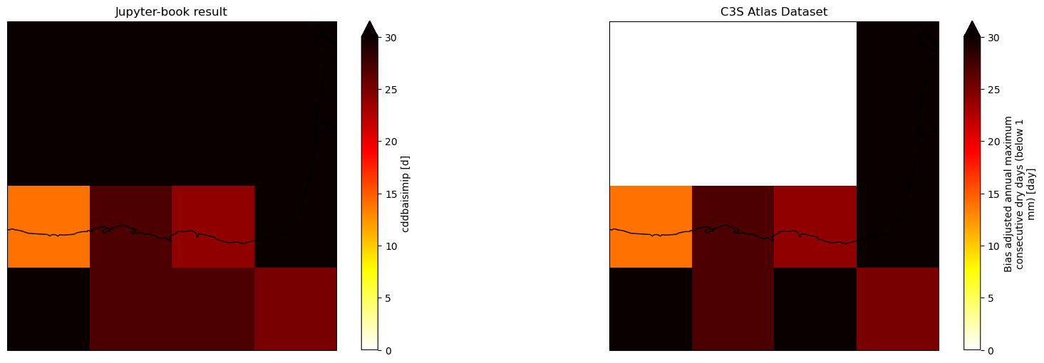
The results are identical, but we have to be careful because the ISIMIP method returns values even in those cells where we do not have data in the reference dataset.