
2.1. Customized regions#
This notebook reproduces the functionalities of the C3S Atlas (https://atlas.climate.copernicus.eu/atlas) for data masking based on customized_regions. This functionality is particularly useful for selecting and analyzing specific geographical areas within the data. The customized_regions function supports five types of regions:
User-defined regions: These are custom regions defined by the user based on specific criteria or geographic boundaries.
AR6 regions: These are regions defined by the IPCC AR6 WG1, used for climate research and analysis (Iturbide et al. 2020).
European countries: This includes masks for individual European countries, allowing for detailed country-level analysis.
EUCRA regions: These are regions defined by the European Climate Assessment & Dataset project.
GeoJSON files: Custom regions can also be defined using GeoJSON files, which allows for highly customizable geographic boundaries based on external data sources.
Users can use the acronyms available in the regions.json to select a specific region for any of the above types of regions.
Throughout this notebook, we will explore how to create and apply these masks to your datasets, enabling targeted and region-specific data analysis.
2.1.1. Load Python packages and clone and install the c3s-atlas GitHub repository from the ecmwf-projects#
Clone (git clone) the c3s-atlas repository and install them (pip install -e .).
Further details on how to clone and install the repository are available in the requirements section
import os
import xarray as xr
from pathlib import Path
import cdsapi
import requests, zipfile, io

from c3s_atlas.utils import (
    extract_zip_and_delete,
)
from c3s_atlas.customized_regions import (
    Mask
)
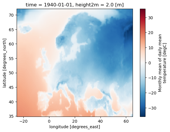
2.1.2. Download climate data with the CDS API#
To reduce data size and download time, a geographical subset focusing on the European region is selected.
cdsapi_url= "https://cds.climate.copernicus.eu/api"
cdsapi_key= ""
c = cdsapi.Client(url=cdsapi_url, key=cdsapi_key)
⚠️ Warning: Exposed API Credentials
For security reasons, it is not recommended to hardcode your Copernicus Climate Data Store (CDS) API credentials — such as
cdsapi_urlandcdsapi_key— directly in notebooks.Instead, it is best to store them securely in a
.cdsapircfile located in your home directory.📄 More info: CDS API - How to use the API
project = "ERA5"
var = 't'
trend_period = period = slice('1991','2020')
dest = Path('./data/ERA5')
os.makedirs(dest, exist_ok=True)
filename = 't_ERA5_mon_194001-202212.zip'

dataset = "multi-origin-c3s-atlas"
request = {
    "origin": "era5",
    "domain": "global",
    "period": "1940-2024",
    "variable": "monthly_temperature",
    "bias_adjustment": "no_bias_adjustment",
    'area': [35, -25, 72, 65], # Europe
}

c.retrieve(dataset, request).download(dest / filename)
extract_zip_and_delete(dest / filename)
ds = xr.open_dataset(dest / "t_ERA5_mon_194001-202212.nc")
# Select firs time step for faster results
ds = ds.isel(time=0)
ds['t'].plot()
<matplotlib.collections.QuadMesh at 0x7baeead22300>
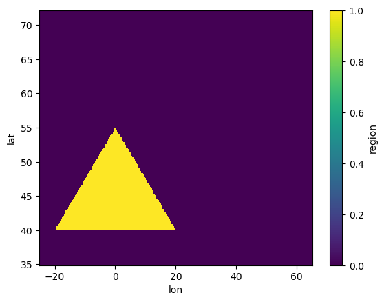
Generate and apply a mask for the user-defined region.#
# Define a triangle mask using coordinates
mask_polygon = Mask(ds).polygon([[-20, 40], [20, 40], [0, 55]])
mask_polygon.plot()
<matplotlib.collections.QuadMesh at 0x7baed89cb980>
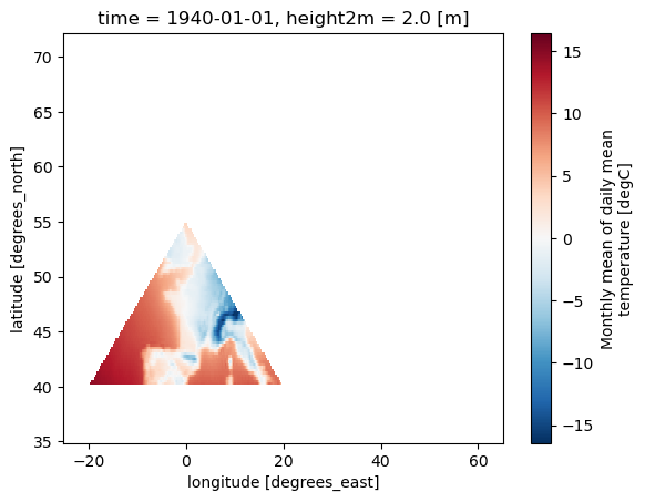
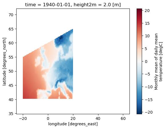
# Mask the dataset (ds) based on the polygon mask (mask_polygon)
ds_masked_polygon = ds.where(mask_polygon)
# Plot the masked dataset (ds_masked_polygon)
ds_masked_polygon[var].plot()
<matplotlib.collections.QuadMesh at 0x7baed87697f0>
# Define a square mask using coordinates (order matters)
mask_polygon = Mask(ds).polygon([[-20, 40], [20, 40], [20, 65], [-20, 55]])
ds_masked_polygon = ds.where(mask_polygon)
ds_masked_polygon[var].plot()
<matplotlib.collections.QuadMesh at 0x7baed8668290>
Generate and apply a mask for the AR6-regions.#
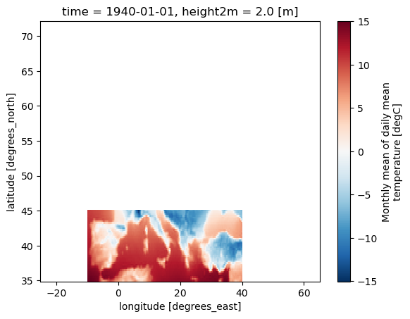
# Create a mask for a specific AR6 region (MED in this case)
mask_AR6 = Mask(ds).regions_AR6(['MED'])
# Mask the dataset (ds) based on the AR6 region mask (mask_AR6)
ds_masked_AR6 = ds.where(mask_AR6)

# Plot the masked dataset for the AR6 region (ds_masked_AR6)
ds_masked_AR6[var].plot()
<matplotlib.collections.QuadMesh at 0x7baed862b3b0>
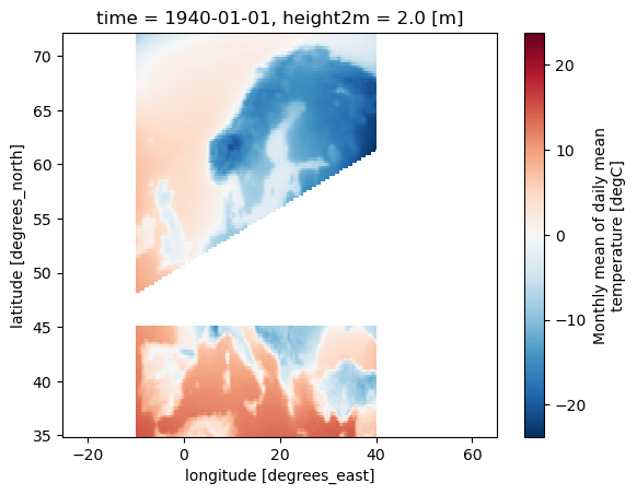
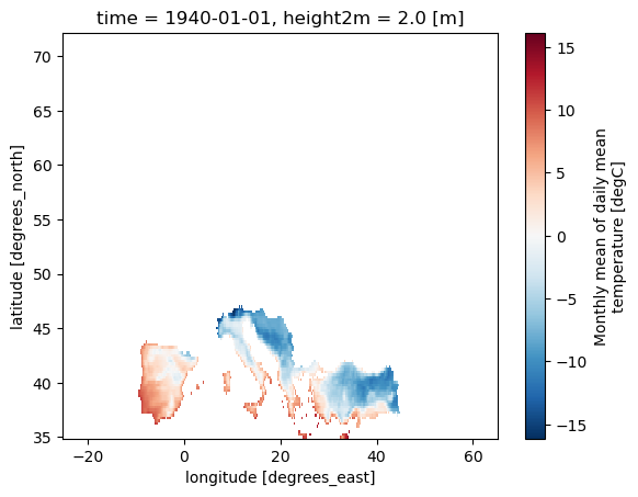
# Define a mask for AR6 regions using a list of region names
mask_AR6 = Mask(ds).regions_AR6(['MED','SAH','NEU'])
ds_masked_AR6 = ds.where(mask_AR6)
ds_masked_AR6[var].plot()
<matplotlib.collections.QuadMesh at 0x7baed82f2d20>
Generate and apply a mask for the European countries.#
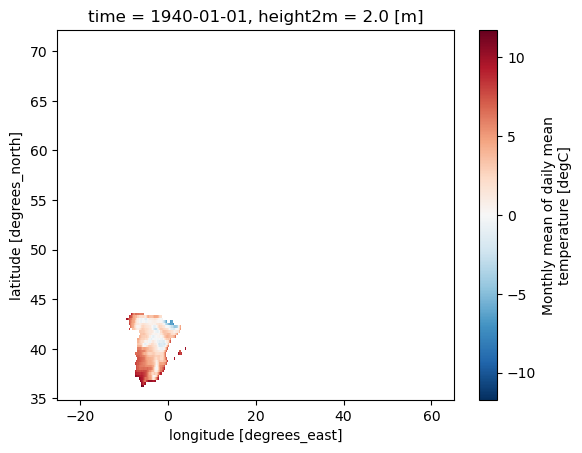
# Define a mask for European countries using a list (including only España)
mask_EUR = Mask(ds).European_contries(['ESP'])
# Mask the dataset (ds) based on the European countries mask (mask_EUR)
ds_masked_EUR = ds.where(mask_EUR)

# Plot the masked dataset for the European countries (ds_masked_EUR)
ds_masked_EUR[var].plot()
<matplotlib.collections.QuadMesh at 0x7baed8781cd0>
# Define a mask for European countries using a list of country abbreviations
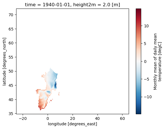
mask_EUR = Mask(ds).European_contries(['ESP','FRA'])
ds_masked_EUR = ds.where(mask_EUR)
ds_masked_EUR[var].plot()
<matplotlib.collections.QuadMesh at 0x7baed7a5d0a0>
Generate and apply a mask for the EUCRA regions.#
# Define a mask for EUCRA areas using a list
mask_EUCRA = Mask(ds).EUCRA_contries(['ST'])
# Mask the dataset (ds) based on the EUCRA countries mask (mask_EUCRA)
ds_masked_EUCRA = ds.where(mask_EUCRA)

# Plot the masked dataset for the EUCRA countries (ds_masked_EUCRA)
ds_masked_EUCRA[var].plot()
<matplotlib.collections.QuadMesh at 0x7baed7b0c290>
# Define a mask for EUCRA countries using a list of abbreviations
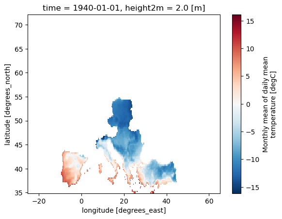
mask_EUCRA = Mask(ds).EUCRA_contries(['ST', 'CT'])
ds_masked_EUCRA = ds.where(mask_EUCRA)
ds_masked_EUCRA[var].plot()
<matplotlib.collections.QuadMesh at 0x7baed825f530>
2.1.3. Download climate data with the CDS API#
project = "ERA5"
var = 't'
trend_period = period = slice('1991','2020')
dest = Path('./data/ERA5')
os.makedirs(dest, exist_ok=True)
filename = 't_ERA5_mon_194001-202212.zip'
dataset = "multi-origin-c3s-atlas"
request = {
"origin": "era5",
"domain": "global",
"period": "1940-2024",
"variable": "monthly_temperature",
"bias_adjustment": "no_bias_adjustment",
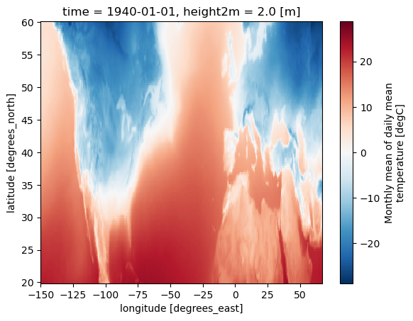
'area': [20, -150, 60, 67], # USA
}
c.retrieve(dataset, request).download(dest / filename)
extract_zip_and_delete(dest / filename)
ds = xr.open_dataset(dest / "t_ERA5_mon_194001-202212.nc")
# Select firs time step for faster results
ds = ds.isel(time=0)
ds['t'].plot()
<matplotlib.collections.QuadMesh at 0x7baed7bbf4d0>
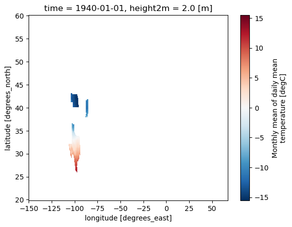
Generate and apply a mask from a different GeoJSON.#
zip_url = "https://download2.exploratory.io/maps/states.zip"
r = requests.get(zip_url)
zip_file = io.BytesIO(r.content)

with zipfile.ZipFile(zip_file, 'r') as zip_ref:
        zip_ref.extractall("./geojsons/")
# Define a mask using a GeoJSON file and names
mask_json = Mask(ds).regions_geojson('./geojsons/states.geojson', "NAME", ["Nebraska", "Indiana", "Texas"])
# Mask the dataset (ds) based on the US states mask (mask_json)
ds_masked_json = ds.where(mask_json)

# Plot the masked dataset for the US states (ds_masked_json)
ds_masked_json[var].plot()
<matplotlib.collections.QuadMesh at 0x7baed7f8f4d0>