
2.2. Geographic Map#
This Jupyter Notebook reproduces the Geographic Map product (see figure bellow) from the C3S Atlas.
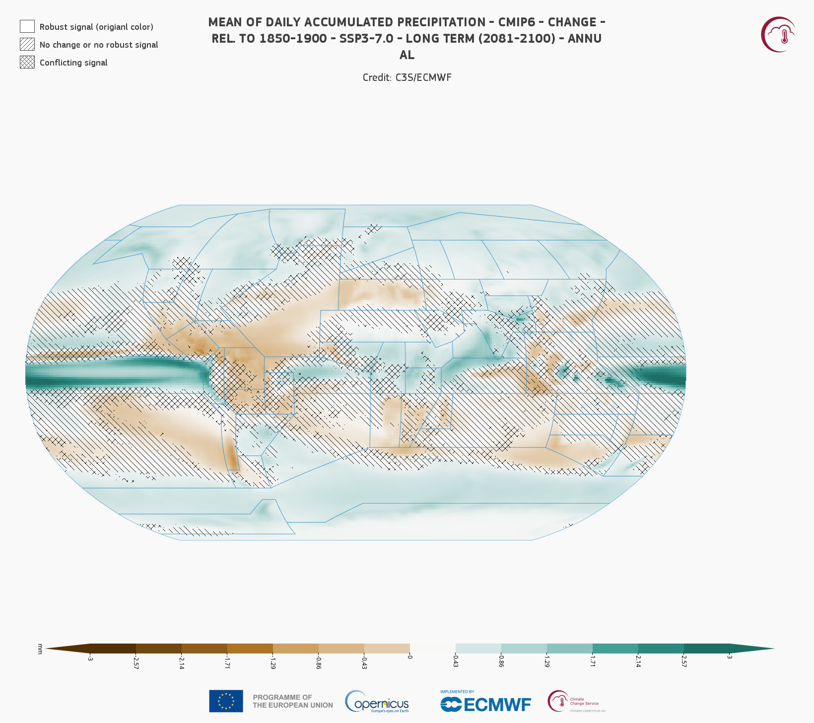
A particular choice of dataset, variable, quantity & scenario and season determines a final product. The bellow figure represents as example the “CMIP6 - Mean of daily accumulated precipitation (mm/day) Change (%) - Warming 2°C SSP5-8.5 (rel. to 1981-2010) - Annual”) which is displayed globally. The map shows the ensemble mean values or changes (absolute or relative –relative changes of the ensemble mean–, depending on the variable). It can be visualized in the C3S Atlas using the following Permalink
To limit the time spent, the spatial map product is calculated for a specific region (Spain)
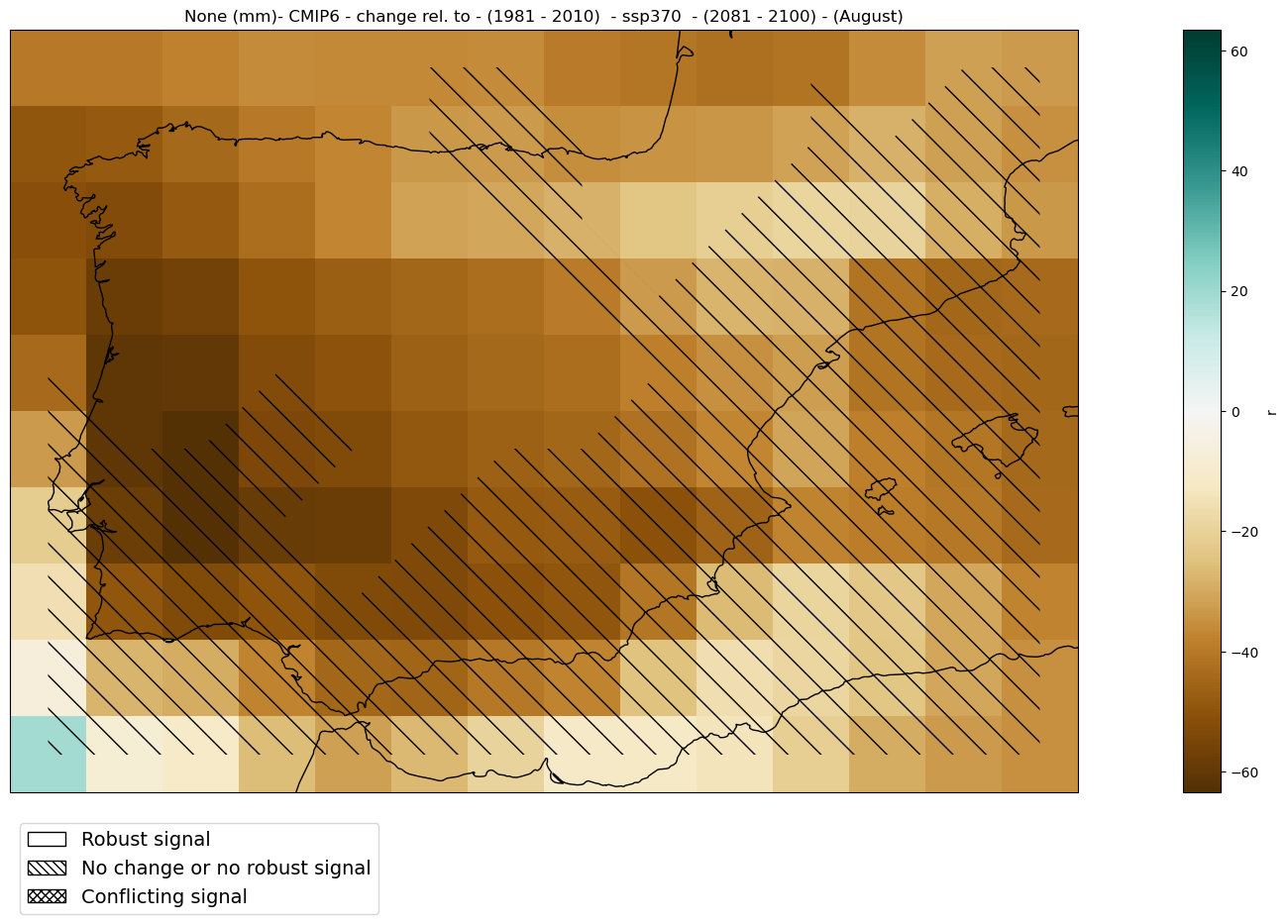
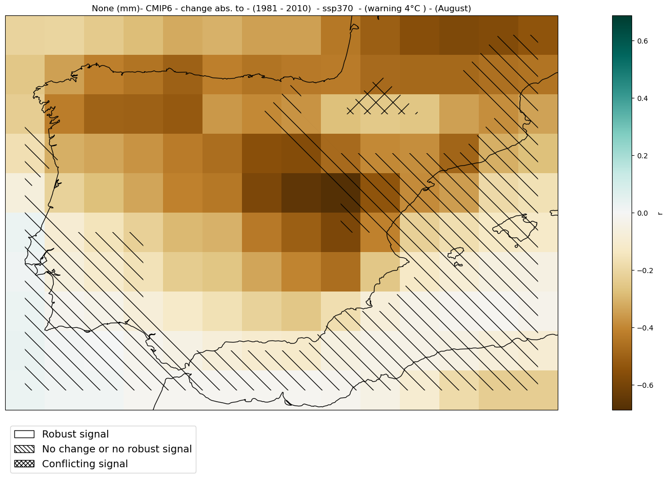
Uncertainty: Visualizing the robustness/uncertainty together with future climate change signals is standard practice to convey comprehensive climate change projections. This information is typically overlaid on the climate change signal using hatching (diagonal lines or crosses obscuring areas with uncertain signals).The advanced method for representing the ensemble robustness of the climate change signal is the approach proposed in AR6. It consists of three categories: 1) robust signal, 2) conflicting signals (crosses overlying the signals), and 3) no change or no robust signal (diagonal lines overlaid on the signal). The first two categories indicate significant changes, i.e. areas where the (20-year mean) climate change model signal likely emerges (individually in >=66% of the models) from the internal variability of 20-year mean values; these changes are defined as robust if at least 80% of the models agree on the sign of change, and as conflicting if less than 80% of the models agree on the sign of change. The third category indicates areas of low change values and/or low significance, where less than 66% of the models exhibit emergent signals. The level of Internal variability (or emergence threshold) was computed as 1.645*sqrt(2/20)*sigma, where 1.645 corresponds to a 90% confidence level and sigma represents the inter-annual standard deviation computed from the linearly detrended baseline period 1971-2005 (IPCC AR6-WGI Atlas; Cross-Chapter Box Atlas.1)
Note that robustness results are computed at a gridbox level and are not representative of regionally aggregated results over larger regions (less influenced by local variability).
2.2.1. Load Python packages and clone and install the c3s-atlas GitHub repository from the ecmwf-projects#
Clone (git clone) the c3s-atlas repository and install them (pip install -e .).
Further details on how to clone and install the repository are available in the requirements section
import xarray as xr
import glob
from datetime import date
import numpy as np
from pathlib import Path
import cdsapi
import os

from c3s_atlas.utils import (
    season_get_name,
    extract_zip_and_delete,
)
from c3s_atlas.customized_regions import (
    Mask
)
from c3s_atlas.analysis import (
    mean_values_map,
    categories_robustness,
    significance_trends,
)
from c3s_atlas.products import (
    hatched_map_plot,
)
from c3s_atlas.GWLs import (
    load_GWLs,
    select_member_GWLs,
    get_mean_data_by_months
)
2.2.2. Download climate data with the CDS API#
To reduce data size and download time, a geographical subset focusing on a specific area within the European region (Spain) is selected.
cdsapi_url= "https://cds.climate.copernicus.eu/api"
cdsapi_key= ""
c = cdsapi.Client(url=cdsapi_url, key=cdsapi_key)
⚠️ Warning: Exposed API Credentials
For security reasons, it is not recommended to hardcode your Copernicus Climate Data Store (CDS) API credentials — such as
cdsapi_urlandcdsapi_key— directly in notebooks.Instead, it is best to store them securely in a
.cdsapircfile located in your home directory.📄 More info: CDS API - How to use the API
project = "CMIP6"
scenario = "ssp370"
var = 'r'
# directory to download the files
dest = Path('./data/CMIP6')
os.makedirs(dest, exist_ok=True)
Download historical scenario#
filename = 'r_CMIP6_historical_mon_185001-201412.zip'
dataset = "multi-origin-c3s-atlas"
request = {
    "origin": "cmip6",
    "experiment": "historical",
    "period": "1850-2014",
    "variable": "monthly_precipitation",
    "bias_adjustment": "no_bias_adjustment",
    'area': [44.5, -9.5, 35.5, 3.5]
}

c.retrieve(dataset, request).download(dest / filename)
extract_zip_and_delete(dest / filename)
Download SSP scenario#
filename = 'r_CMIP6_ssp370_mon_201501-210012.zip'
dataset = "multi-origin-c3s-atlas"
request = {
    "origin": "cmip6",
    "experiment": "ssp3_7_0",
    "period": "2015-2100",
    "variable": "monthly_precipitation",
    "bias_adjustment": "no_bias_adjustment",
    'area': [44.5, -9.5, 35.5, 3.5]
}

c.retrieve(dataset, request).download(dest / filename)
extract_zip_and_delete(dest / filename)
Concatenate historical and SSP scenarios#
Note that the historical and SSP scenarios may have a different number of members. Here, common members from the historical and SSP scenarios are concatenated into a single xarray.Dataset to facilitate their use going forward.
ds_hist = xr.open_dataset(dest / "r_CMIP6_historical_mon_185001-201412.nc")
ds_sce = xr.open_dataset(dest / "r_CMIP6_ssp370_mon_201501-210012.nc")
mem_inters = np.intersect1d(ds_hist.member_id.values, ds_sce.member_id.values)
ds_hist = ds_hist.isel(member = np.isin(ds_hist.member_id.values, mem_inters))
ds_sce = ds_sce.isel(member = np.isin(ds_sce.member_id.values, mem_inters))
ds = xr.concat([ds_hist, ds_sce], dim = 'time')
Define season#
We select month 8 (August) as an example to viusalize the results#
season = [8] # Months
attrs = {
    "project" : project,
    "scenario": scenario,
    "variable": var,
    "season": season,
    "season_name" : season_get_name(season),
    "actual_year": date.today().year,
    "unit" : ds[var].units
}
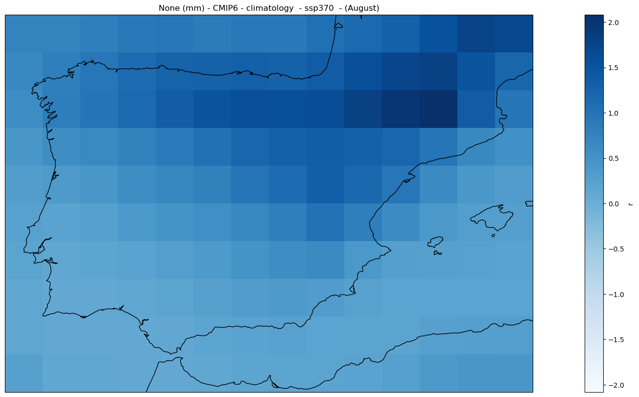
2.2.3. Climatology#
Analysis#
The mean_values_map function calculates the mean value over the time dimension for a specific period.
mode = 'climatology'
period = slice('2081', '2100')
mean_map_ds = mean_values_map(ds, var, project, mode = mode,
                              season = season, period = period)
Plot#
fig = hatched_map_plot(mean_map_ds, var, attrs, mode = 'climatology', cmap = 'Blues')
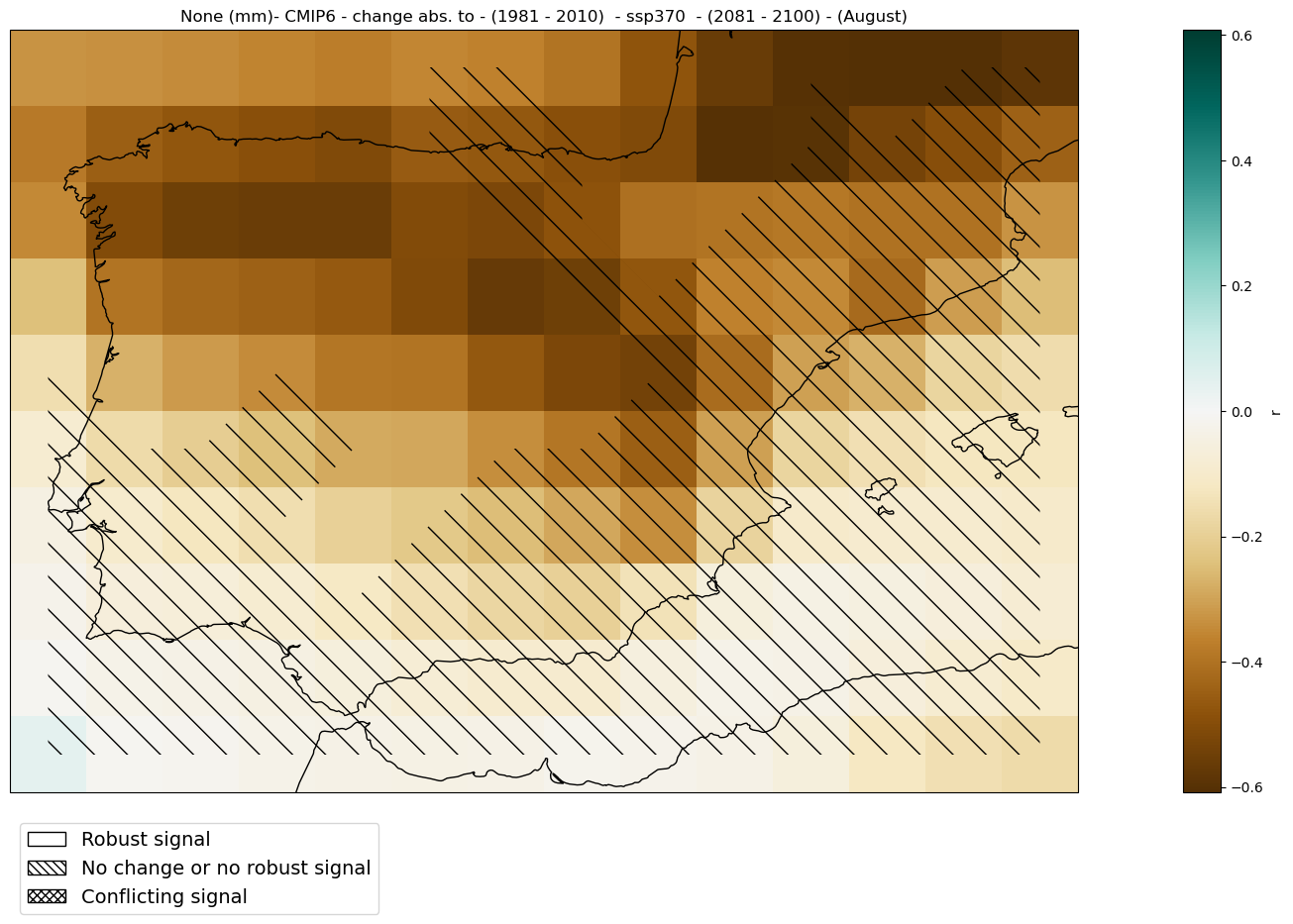
2.2.4. Absolute change#
Analysis#
The categories_robustness function calculate the category of robustness of the climate signal for each gridbox, using the same approaches as those in the IPCC WGI AR6 report (Cross-Chapter Box Atlas.1).
mode = 'change'
diff = 'abs'
period = slice('2081', '2100')
baseline_period = slice('1981', '2010')
mean_map_ds = mean_values_map(ds, var, project, mode = mode, diff = diff,
                              season = season, period = period,
                              baseline_period = baseline_period)
# calculate robusteness
# Note that this product is time-cosuming and can take several minutes
categories_ds = categories_robustness(ds, var, season = season,
                                      period = period,
                                      baseline_period = baseline_period)
Plot#
fig = hatched_map_plot(mean_map_ds, var, attrs,
                       mode = mode, diff = diff,
                       categories = categories_ds[0],
                       period = period, baseline_period = baseline_period,
                       cmap = 'BrBG')
2.2.5. Relative Change#
mode = 'change'
diff = 'rel'
period=slice('2081', '2100')
baseline_period=slice('1981', '2010')
mean_map_ds = mean_values_map(ds, var, project, mode = mode, diff = diff,
                              season = season, period = period,
                              baseline_period = baseline_period)
# The robustness analysis is indifferent to the mode (abs/rel)
#categories_ds = categories_robustness(ds, var, months = season,
#                                      period = period,
#                                      baseline_period = baseline_period)
Plot#
fig = hatched_map_plot(mean_map_ds, var, attrs,
                       mode = mode, diff = diff,
                       categories = categories_ds[0],
                       period = period, baseline_period = baseline_period,
                       cmap = 'BrBG')
2.2.6. Global Warming Levels#
Here, the spatial map is displayed for a specific Global Warming Level (GWL). To achieve this, the 20-year period in which each ensemble member reaches the chosen GWL is selected. The spatial map is then shown, representing either climatology or change for this specific period and region (Spain in this notebook).
These periods are calculated in the notebook GWLs.ipynb for CMIP5 and CMIP6. For CORDEX, the results from the driving CMIP5 models are used.
GWL = '4'
#Load the data and get the intersection of the members
GWLs_ds = load_GWLs(project)
GWLs_members_with_period = select_member_GWLs(ds, GWLs_ds, project, scenario, GWL)
[GWL_data, filtered_GWLs_ds]=get_mean_data_by_months(ds, GWLs_members_with_period)
Analysis#
mode = 'change'
diff = 'abs'
baseline_period = slice('1981', '2010')
mean_map_ds = mean_values_map(filtered_GWLs_ds, var, project, mode = mode,
                            diff = diff, season = season,
                            baseline_period = baseline_period, GWLs_ds = GWL_data)
categories_ds = categories_robustness(filtered_GWLs_ds, var, season = season,
                                       baseline_period =  baseline_period,
                                       GWLs_ds = GWL_data)
Plot#
hatched_map_plot(mean_map_ds, var, attrs, mode = mode, diff = diff,
                 categories = categories_ds[0],
                 baseline_period = baseline_period, GWLs = GWL,
                 cmap = 'BrBG')
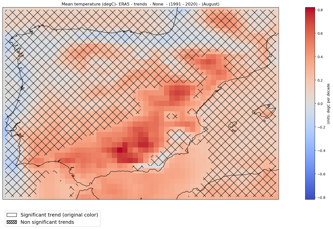
2.2.7. Trends#
Trend analysis is only available for observations and reanalysis. This type of analysis is not appropriate for projections since climate change does not necessarily scale linearly with global warming.
Download data from the “Gridded dataset underpinning the Copernicus Interactive Climate Atlas”#
project = "ERA5"
var = 't'
season = [8]
trend_period = period = slice('1991','2020')
dest = Path('./data/ERA5')
os.makedirs(dest, exist_ok=True)
filename = 't_ERA5_mon_194001-202212.zip'

dataset = "multi-origin-c3s-atlas"
request = {
    "origin": "era5",
    "domain": "global",
    "period": "1940-2024",
    "variable": "monthly_temperature",
    "bias_adjustment": "no_bias_adjustment",
    'area': [44.5, -9.5, 35.5, 3.5]
}

c.retrieve(dataset, request).download(dest / filename)
extract_zip_and_delete(dest / filename)
ds = xr.open_dataset(dest / "t_ERA5_mon_194001-202212.nc")
attrs = {
    "project" : project,
    "variable": var,
    "season": season,
    "season_name" : season_get_name(season),
    "actual_year": date.today().year,
    "unit" : ds[var].units
}
Analysis#
The significance_trends function calculates and returns p-values for linear regression trends for each latitude-longitude point. Robustness is defined using the significance of the linear trends as obtained from standard hypothesis testing (and obscuring regions with non-significant trends using “x”).
A p-value indicates the level of significance of the trend:
A small p-value (usually less than 0.05) means it’s very unlikely to be random — so we can trust the trend is significant.
A large p-value means the trend might just be noise or coincidence, so we don’t consider it reliable.
ds = significance_trends(ds, var, season, trend_period = trend_period)
Plot#
mode = 'trends'
pvalue = 0.05 # level of significance
hatched_map_plot(ds, var, attrs, mode = mode,
                 period = period, pvalue = 0.05, cmap = 'coolwarm')