Please note that this repository is used for development and review, so quality assessments should be considered work in progress until they are merged into the main branch

7.2. Consistency between the C3S Atlas dataset and its origins: Multiple indicators

Production date: 2025-10-01.

Dataset version: 2.0.

Produced by: Olivier Burggraaff, Nicole Reynolds (National Physical Laboratory).

🌍 Use case: Retrieving climate indicators from the Copernicus Interactive Climate Atlas

❓ Quality assessment question

• Are the climate indicators in the dataset underpinning the Copernicus Interactive Climate Atlas consistent with their origin datasets?

• Can the dataset underpinning the Copernicus Interactive Climate Atlas be reproduced from its origin datasets?

The Copernicus Interactive Climate Atlas, or C3S Atlas for short, is a C3S web application providing an easy-to-access tool for exploring climate projections, reanalyses, and observational data [Gutiérrez+24]. Version 2.0 of the application allows the user to interact with 12 datasets:

Type	Dataset
Climate Projection	CMIP6
Climate Projection	CMIP5
Climate Projection	CORDEX-CORE
Climate Projection	CORDEX-EUR-11
Reanalysis	ERA5
Reanalysis	ERA5-Land
Reanalysis	ORAS5
Reanalysis	CERRA
Observations	E-OBS
Observations	BERKEARTH
Observations	CPC
Observations	SST-CCI

These datasets are provided through an intermediary dataset, the Gridded dataset underpinning the Copernicus Interactive Climate Atlas or C3S Atlas dataset for short [C3S Atlas dataset]. Compared to their origins, the versions of the climate datasets within the C3S Atlas dataset have been processed following the workflow in Figure 7.2.1.

Fig. 7.2.1 Schematic representation of the workflow for the production of the C3S Atlas dataset from its origin datasets, from the User-tools for the C3S Atlas.

Because a wide range of users interact with climate data through the C3S Atlas application, it is crucial that the underpinning dataset represent its origins correctly. In other words, the C3S Atlas dataset must be consistent with and reproducible from its origins. Here, we assess this consistency and reproducibility by comparing climate indicators retrieved from the C3S Atlas dataset with their equivalents calculated from the origin dataset, mirroring the workflow from Figure 7.2.1. While a full analysis and reproduction of every record within the C3S Atlas dataset is outside the scope of quality assessment (and would require high-performance computing infrastructure), a case study with a narrower scope probes these quality attributes of the dataset and can be a jumping-off point for further analysis by the reader.

This notebook is part of a series:

Notebook	Contents
Consistency between the C3S Atlas dataset and its origins: Case study	Comparison between C3S Atlas dataset and one origin dataset (CMIP6) for one indicator (tx35), including detailed setup.
Consistency between the C3S Atlas dataset and its origins: Multiple indicators	Comparison between C3S Atlas dataset and one origin dataset (CMIP6) for multiple indicators.
Consistency between the C3S Atlas dataset and its origins: Multiple origin datasets	Comparison between C3S Atlas dataset and multiple origin datasets for one indicator.

📢 Quality assessment statement

These are the key outcomes of this assessment

• Climate indicators (here 25 monthly indicators) provided by the C3S Atlas dataset are highly consistent with values calculated from its origin datasets (here the CMIP6 multi-model ensemble).

• There are some differences in coverage between the C3S Atlas dataset and its origins due to deliberate masking, e.g. agricultural indicators in the Arctic circle, but these do not affect the vast majority use cases for the C3S Atlas.

• Differences between the C3S Atlas dataset and a manual reproduction are rare and generally negligible (median absolute difference ≤0.02% for all but 2 indicators). Where differences occur, they can be explained by details of the workflow implementation or deliberate choices.

• The C3S Atlas is traceable and reproducible, and can be confidently used to view, analyse, and download climate data.

• For specific use cases, like scientific papers, it is recommended to manually process the origin dataset instead of using the C3S Atlas. This is not necessary for other use cases, such as climate risk assessments and climate reports, in which case the C3S Atlas can be used as is.

📋 Methodology

This quality assessment tests the consistency between climate indicators retrieved from the Gridded dataset underpinning the Copernicus Interactive Climate Atlas [C3S Atlas dataset] and their equivalents calculated from the origin datasets, as well as the reproducibility of said dataset.

This notebook expands the analysis set out in the case study to investigate multiple indicators (listed below, descriptions from the User-tools for the C3S Atlas) derived from the CMIP6 multi-model ensemble [CMIP6 dataset]:

Indicator	Unit	Full description
t	°C	Monthly mean of daily mean near-surface (2-metre) air temperature
tn	°C	Monthly mean of daily minimum near-surface (2-metre) air temperature
tx	°C	Monthly mean of daily maximum near-surface (2-metre) air temperature
dtr	°C	Monthly mean of near-surface (2-metre) air temperature difference between the maximum and minimum daily temperature
tnn	°C	Monthly minimum of daily minimum near-surface (2-metre) air temperature
txx	°C	Monthly maximum of daily maximum near-surface (2-metre) air temperature
tx35	d	Monthly count of days with maximum near-surface (2-metre) temperature above 35 °C
tx40	d	Monthly count of days with maximum near-surface (2-metre) temperature above 40 °C
tr	d	Monthly count of tropical nights (days with minimum temperature above 20 °C)
fd	d	Monthly count of days with minimum near-surface (2-metre) temperature below 0 °C
r	mm	Monthly mean of daily accumulated precipitation of liquid water equivalent from all phases
sdii	mm	Monthly average of daily precipitation amount of liquid water equivalent from all phases on days with precipitation amount above or equal to 1 mm
prsn	mm	Monthly mean of daily accumulated liquid water equivalent thickness snowfall
rx1day	mm	Monthly maximum of 1-day accumulated precipitation of liquid water equivalent from all phases
r01	d	Monthly count of days with daily accumulated precipitation of liquid water equivalent from all phases above 1 mm
r10	d	Monthly count of days with daily accumulated precipitation of liquid water equivalent from all phases above 10 mm
r20	d	Monthly count of days with daily accumulated precipitation of liquid water equivalent from all phases above 20 mm
pet	mm	Monthly mean daily accumulated potential evapotranspiration (Hargreaves method, 1985), which is the rate at which evapotranspiration would occur under ambient conditions from a uniformly vegetated area when the water supply is not limiting
evspsbl	mm	Monthly mean of daily amount of water in the atmosphere due to conversion of both liquid and solid phases to vapor (from underlying surface and vegetation)
huss	g/kg	Monthly amount of moisture in the air near the surface divided by amount of air plus moisture at that location
psl	hPa	Monthly average air pressure at mean sea level
sfcwind	m/s	Monthly mean of daily mean near-surface (10-metre) wind speed
clt	%	Monthly mean cloud cover area percentage
rsds	W/m²	Monthly mean incident solar (shortwave) radiation that reaches a horizontal plane at the surface
rlds	W/m²	Monthly mean incident thermal (longwave) radiation at the surface (during cloudless and overcast conditions)

The analysis and results are organised in the following steps, which are detailed in the sections below:

1. Code setup

• Install User-tools for the C3S Atlas.

• Import all required libraries.

• Define indicators.

• Define helper functions.

2. Calculate indicators from the origin dataset

• Download data from the origin dataset(s).

• Homogenise data.

• Calculate indicator(s).

• Regrid the origin data to the C3S Atlas grid.

3. Retrieve indicators from the C3S Atlas dataset

• Download data from the C3S Atlas dataset.

4. Results

• Consistency: Compare the C3S Atlas and reproduced datasets on native grids.

• Reproducibility: Compare the C3S Atlas and reproduced datasets on the C3S Atlas grid.

📈 Analysis and results

1. Code setup

Note

This notebook uses earthkit for downloading (earthkit-data) and visualising (earthkit-plots) data. Because earthkit is in active development, some functionality may change after this notebook is published. If any part of the code stops functioning, please raise an issue on our GitHub repository so it can be fixed.

Install the User-tools for the C3S Atlas

This notebook uses the User-tools for the C3S Atlas, which can be installed from GitHub using pip. For convenience, the following cell can do this from within the notebook. Further details and alternative options for installing this library are available in its documentation.

Show code cell source

Hide code cell source

!pip install git+https://github.com/ecmwf-projects/c3s-atlas.git

Import required libraries

In this section, we import all the relevant packages needed for running the notebook.

Show code cell source

Hide code cell source

# Input / Output
from pathlib import Path
import earthkit.data as ekd
import warnings

# General data handling
import numpy as np
np.seterr(divide="ignore")  # Ignore divide-by-zero warnings
import pandas as pd
import xarray as xr
from functools import partial
from dask.array.core import PerformanceWarning
warnings.simplefilter(action="ignore", category=PerformanceWarning)

# Data pre-processing
from c3s_atlas.fixers import apply_fixers
import c3s_atlas.interpolation as xesmfCICA

# Climate indicators
import xclim
xclim.set_options(cf_compliance="log")  # Mute warnings
import c3s_atlas.indexes

# Fix for bug affecting sfcWind units
from c3s_atlas.units import VALID_UNITS
VALID_UNITS["sfcWind"] = r"(m s-1|m s\^-1|m/s)"

# Visualisation
import earthkit.plots as ekp
from earthkit.plots.styles import Style
import matplotlib.pyplot as plt
plt.rcParams["grid.linestyle"] = "--"
from tqdm import tqdm  # Progress bars

# Visualisation in Jupyter book -- automatically ignored otherwise
try:
    from myst_nb import glue
except ImportError:
    glue = None

# Type hints
from typing import Iterable, Optional
from earthkit.plots.geo.domains import Domain
AnyDomain = (Domain | str)

Define indicators

This section defines functions and variables for calculating and using the climate indicators. These are split into three cells, corresponding to their input and output data types.

Daily data → Monthly indicators:

Show code cell source

Hide code cell source

# Daily data -> Monthly indicators
# Input: tas
def cal_t(ds: xr.Dataset) -> xr.Dataset:
    """ Monthly mean of daily mean near-surface (2-metre) air temperature """
    ds_t = ds['tas'].resample(time='MS').mean().to_dataset(name='t')
    return ds_t

# Input: tasmin
def cal_tn(ds: xr.Dataset) -> xr.Dataset:
    """ Monthly mean of daily minimum near-surface (2-metre) air temperature """
    ds_tn = ds['tasmin'].resample(time='MS').mean().to_dataset(name='tn')
    return ds_tn 

def cal_tnn(ds: xr.Dataset) -> xr.Dataset:
    """ Monthly minimum of daily minimum near-surface (2-metre) air temperature """
    ds_tnn = ds['tasmin'].resample(time='MS').min().to_dataset(name='tnn')
    return ds_tnn

def cal_tr(ds: xr.Dataset) -> xr.Dataset:
    """ Monthly count of tropical nights (days with minimum temperature above 20 degC) """
    ds_tr = xclim.indicators.atmos.tropical_nights(ds['tasmin'], thresh='20.0 degC', freq='MS', op='>').to_dataset(name='tr')
    return ds_tr

def cal_fd(ds: xr.Dataset) -> xr.Dataset:
    """ Monthly count of days with minimum near-surface (2-metre) temperature below 0 °C """
    ds_fd = xclim.indicators.atmos.frost_days(ds['tasmin'], thresh='0 degC', freq='MS').to_dataset(name='fd')
    return ds_fd

# Input: tasmax
def cal_tx(ds: xr.Dataset) -> xr.Dataset:
    """ Monthly mean of daily maximum near-surface (2-metre) air temperature """
    ds_tx = ds['tasmax'].resample(time='MS').mean().to_dataset(name='tx')
    return ds_tx

def cal_txx(ds: xr.Dataset) -> xr.Dataset:
    """ Monthly maximum of daily maximum near-surface (2-metre) air temperature """
    ds_txx = ds['tasmax'].resample(time='MS').max().to_dataset(name='txx')
    return ds_txx

def cal_tx35(ds: xr.Dataset) -> xr.Dataset:
    """ Monthly count of days with maximum near-surface (2-metre) temperature above 35 °C """
    ds_tx35 = xclim.indices.tx_days_above(ds['tasmax'], thresh='35.0 degC', freq='MS', op='>').to_dataset(name='tx35')
    return ds_tx35

def cal_tx40(ds: xr.Dataset) -> xr.Dataset:
    """ Monthly count of days with maximum near-surface (2-metre) temperature above 40 °C """
    ds_tx40 = xclim.indices.tx_days_above(ds['tasmax'], thresh='40.0 degC', freq='MS', op='>').to_dataset(name='tx40')
    return ds_tx40

# Input: tasmin + tasmax
def cal_dtr(ds: xr.Dataset) -> xr.Dataset:
    """ Monthly mean of near-surface (2-metre) air temperature difference between the maximum and minimum daily temperature """
    ds_dtr = xclim.indices.daily_temperature_range(ds['tasmin'], ds['tasmax'], freq='MS', op='mean').to_dataset(name='dtr')
    return ds_dtr

# Input: pr
def cal_r(ds: xr.Dataset) -> xr.Dataset:
    """ Monthly mean of daily accumulated precipitation of liquid water equivalent from all phases """
    ds_r = ds['pr'].resample(time='MS').mean().to_dataset(name='r')
    return ds_r

def cal_r01(ds: xr.Dataset) -> xr.Dataset:
    """ Monthly count of days with daily accumulated precipitation of liquid water equivalent from all phases above 1 mm """
    pr_flux = ds['pr'].copy().assign_attrs(units = 'mm/day')
    per0 = xr.zeros_like(pr_flux).assign_attrs(units='mm/day')
    ds_r01 = xclim.indices.days_over_precip_thresh(pr_flux, per0, thresh='1 mm/day', freq='MS', bootstrap=False, op='>').to_dataset(name='r01')
    return ds_r01

def cal_sdii(ds: xr.Dataset) -> xr.Dataset:
    """ Monthly average of daily precipitation amount of liquid water equivalent from all phases on days with precipitation amount above or equal to 1 mm """
    pr_flux = ds['pr'].copy().assign_attrs(units = 'mm/day')
    ds_sdii = xclim.indicators.atmos.daily_pr_intensity(pr_flux, thresh='1 mm/day', freq='MS', op='>=').to_dataset(name='sdii')
    return ds_sdii

def cal_r10(ds: xr.Dataset) -> xr.Dataset:  
    """ Monthly count of days with daily accumulated precipitation of liquid water equivalent from all phases above 10 mm """
    pr_flux = ds['pr'].copy().assign_attrs(units = 'mm/day')
    per0 = xr.zeros_like(pr_flux).assign_attrs(units='mm/day')
    ds_r10 = xclim.indices.days_over_precip_thresh(pr_flux, per0, thresh='10 mm/day', freq='MS', bootstrap=False, op='>').to_dataset(name='r10')
    return ds_r10

def cal_r20(ds: xr.Dataset) -> xr.Dataset:
    """ Monthly count of days with daily accumulated precipitation of liquid water equivalent from all phases above 20 mm """
    pr_flux = ds['pr'].copy().assign_attrs(units = 'mm/day')
    per0 = xr.zeros_like(pr_flux).assign_attrs(units='mm/day')
    ds_r20 = xclim.indices.days_over_precip_thresh(pr_flux, per0, thresh='20 mm/day', freq='MS', bootstrap=False, op='>').to_dataset(name='r20')
    return ds_r20

def cal_rx1day(ds: xr.Dataset) -> xr.Dataset:
    """ Monthly maximum of 1-day accumulated precipitation of liquid water equivalent from all phases """
    pr_flux = ds['pr'].copy().assign_attrs(units = 'mm/day')
    ds_rx1day = xclim.indicators.atmos.max_n_day_precipitation_amount(pr_flux, window=1, freq='MS').to_dataset(name='rx1day')
    return ds_rx1day

# Input: pet
def cal_pet(ds: xr.Dataset) -> xr.Dataset:
    """ Monthly mean daily accumulated potential evapotranspiration (Hargreaves method, 1985), which is the rate at which evapotranspiration would occur under ambient conditions from a uniformly vegetated area when the water supply is not limiting """
    ds_pet = xclim.indices.potential_evapotranspiration(ds['tasmin'], ds['tasmax'], method='HG85').resample(time='MS').mean().to_dataset(name='pet')
    # Convert to mm (assuming kg water /m² = mm)
    ds_pet["pet"] *= 86400
    ds_pet["pet"] = ds_pet["pet"].assign_attrs({"units": "mm"})
    return ds_pet

# Input: huss
def cal_huss(ds: xr.Dataset) -> xr.Dataset:
    """ Monthly amount of moisture in the air near the surface divided by amount of air plus moisture at that location """
    ds_huss = ds['huss'].resample(time='MS').mean().to_dataset(name='huss')
    # Convert to g/kg
    ds_huss["huss"] *= 1000
    ds_huss["huss"] = ds_huss["huss"].assign_attrs({"units": "gr kg-1"})
    return ds_huss

# Defunct -- problems with units
# def cal_rx5day(ds: xr.Dataset) -> xr.Dataset:
#     """ Monthly maximum of 5-day accumulated precipitation of liquid water equivalent from all phases """
#     pr_flux = ds['pr'].copy().assign_attrs(units = 'mm/day')
#     ds_rx5day = xclim.indicators.atmos.max_n_day_precipitation_amount(pr_flux, window=5, freq='MS').to_dataset(name='rx5day')
#     return ds_rx5day

# def cal_spi6(ds: xr.Dataset) -> xr.Dataset:
#     """ Monthly index that compares accumulated precipitation for 6 months with the long-term precipitation distribution for the same location and accumulation period, as the number of standard deviations from the mean. The reference period corresponds to 1971-2010 """
#     pr_flux = ds['pr'].copy().assign_attrs(units = 'mm/day')
#     ds_spi6 = xclim.indices.standardized_precipitation_index(pr_flux, freq='MS', window=6, dist='gamma', method='ML').to_dataset(name='spi6')
#     return ds_spi6

# def cal_spei6(ds: xr.Dataset) -> xr.Dataset:
#      """ Monthly index that compares accumulated precipitation minus potential evapotranspiration (Hargreaves method, 1985) for 6 months with the long-term distribution for the same location and accumulation period, as the number of standard deviations from the mean. The reference period corresponds to 1971-2010 """
#     pr_flux = ds['pr'].copy().assign_attrs(units = 'mm/day')
#     ds_spei6 = xclim.indices.standardized_precipitation_index(pr_flux, freq='MS', window=6, dist='gamma', method='ML').to_dataset(name='spei6')
#     return ds_spei6

Monthly data → Monthly indicators:

Show code cell source

Hide code cell source

# Monthly data -> Monthly indicators
# Input: evpsbl
def cal_evspsbl(ds: xr.Dataset) -> xr.Dataset:
    """ Monthly mean of daily amount of water in the atmosphere due to conversion of both liquid and solid phases to vapor (from underlying surface and vegetation) """
    ds_evspsbl = ds['evspsbl'].resample(time='MS').mean().to_dataset(name='evspsbl')
    return ds_evspsbl

# Input: mrsos
def cal_mrsos(ds: xr.Dataset) -> xr.Dataset:
    """ Monthly soil shallow moisture content, as the vertical sum per unit area of water in all phases contained in the upper soil portion to a depth of 7 to 10 cm (depending on the dataset) """
    ds_mrsos = ds['mrsos'].resample(time='MS').mean().to_dataset(name='mrsos')
    return ds_mrsos

# Input: mrro
def cal_mrro(ds: xr.Dataset) -> xr.Dataset:
    """ Monthly mean of daily amount per unit area of surface and subsurface liquid water which drains from land """
    ds_mrro = ds['mrro'].resample(time='MS').mean().to_dataset(name='mrro')
    return ds_mrro

# Input: prsn
def cal_prsn(ds: xr.Dataset) -> xr.Dataset:
    """ Monthly mean of daily accumulated liquid water equivalent thickness snowfall """
    ds_prsn = ds['prsn'].resample(time='MS').mean().to_dataset(name='prsn')
    return ds_prsn

# Input: sfcWind
def cal_sfcwind(ds: xr.Dataset) -> xr.Dataset:
    """ Monthly mean of daily mean near-surface (10-metre) wind speed """
    ds_sfcwind = ds['sfcWind'].resample(time='MS').mean().to_dataset(name='sfcwind')
    return ds_sfcwind

# Input: clt
def cal_clt(ds: xr.Dataset) -> xr.Dataset:
    """ Monthly mean cloud cover area percentage """
    ds_clt = ds['clt'].resample(time='MS').mean().to_dataset(name='clt')
    return ds_clt

# Input: rsds
def cal_rsds(ds: xr.Dataset) -> xr.Dataset:
    """ Monthly mean incident solar (shortwave) radiation that reaches a horizontal plane at the surface """
    ds_rsds = ds['rsds'].resample(time='MS').mean().to_dataset(name='rsds')
    return ds_rsds

# Input: rlds
def cal_rlds(ds: xr.Dataset) -> xr.Dataset:
    """ Monthly mean incident thermal (longwave) radiation at the surface (during cloudless and overcast conditions) """
    ds_rlds = ds['rlds'].resample(time='MS').mean().to_dataset(name='rlds')
    return ds_rlds

# Input: psl
def cal_psl(ds: xr.Dataset) -> xr.Dataset:
    """ Monthly average air pressure at mean sea level """
    ds_psl = ds['psl'].resample(time='MS').mean().to_dataset(name='psl')
    # Convert to hPa
    ds_psl["psl"] /= 100
    ds_psl["psl"] = ds_psl["psl"].assign_attrs({"units": "hPa"})
    return ds_psl

Monthly data → Yearly indicators. These yearly indicators are not used in the rest of the analysis, but are included as a jumping-off point for the reader’s own analysis.

Show code cell source

Hide code cell source

# Daily data -> Yearly indicators
# Input: pr
def cal_cdd(ds: xr.Dataset) -> xr.Dataset:
    """ Annual maximum of consecutive days when daily accumulated precipitation amount is below 1 mm """
    pr_flux = ds['pr'].copy().assign_attrs(units = 'mm/day')
    ds_cdd = xclim.indicators.atmos.maximum_consecutive_dry_days(pr_flux, thresh='1 mm/day', freq='YS', resample_before_rl=True).to_dataset(name='cdd')
    return ds_cdd

# Input: tas + tasmin + tasmax
def cal_hd(ds: xr.Dataset) -> xr.Dataset:
    """ Annual energy consumption to heat the deficit of temperature below 15.5 °C """
    ds_hd = c3s_atlas.indexes.heating_degree_days(ds['tas'], ds['tasmax'], ds['tasmin'], freq='YS', thresh=15.5).to_dataset(name='hd')
    return ds_hd

def cal_cd(ds: xr.Dataset) -> xr.Dataset:
    """ Annual energy consumption to cool the excess of temperature above 22 °C """
    ds_cd = c3s_atlas.indexes.cooling_degree_days(ds['tas'], ds['tasmax'], ds['tasmin'], freq='YS', thresh=22).to_dataset(name='cd')
    return ds_cd

The following cell defines some convenience functions for calculating multiple indicators in a loop, grouped according to their input and output data types:

Show code cell source

Hide code cell source

# Combine functions into dictionaries for easy access by name
indicators_daily2monthly = {
    "t": cal_t,
    "tn": cal_tn,
    "tx": cal_tx,
    "dtr": cal_dtr,
    "tnn": cal_tnn,
    "txx": cal_txx,
    "tx35": cal_tx35,
    "tx40": cal_tx40,
    "tr": cal_tr,
    "fd": cal_fd,
    "r": cal_r,
    "sdii": cal_sdii,
    "rx1day": cal_rx1day,
    "r01": cal_r01,
    "r10": cal_r10,
    "r20": cal_r20,
    # Note: Skipping rx5day due to window length error
    # "rx5day": cal_rx5day,
    # Note: Skipping spi6, spei6 due to unit issues
    # "spi6": cal_spi6,
    # "spei6": cal_spei6,
    "pet": cal_pet,
    "huss": cal_huss,
}

indicators_monthly2monthly = {
    "prsn": cal_prsn,
    "evspsbl": cal_evspsbl,
    # Note: Skipping mrsos and mrro due to CMIP6 grid issues
    # "mrsos": cal_mrsos,
    # "mrro": cal_mrro,
    "psl": cal_psl,
    "sfcwind": cal_sfcwind,
    "clt": cal_clt,
    "rsds": cal_rsds,
    "rlds": cal_rlds,
}

indicators_daily2annual = {
    "cdd": cal_cdd,
    "hd": cal_hd,
    "cd": cal_cd,
}

# Easier access in loops
indicators_monthly = indicators_daily2monthly | indicators_monthly2monthly
indicators_annual  = indicators_daily2annual
indicators         = indicators_daily2monthly | indicators_monthly2monthly | indicators_daily2annual

# Hard-code monthly indicator names to match table in intro
indicators_monthly_names = [
    "t", "tn", "tx", "dtr", "tnn", "txx", "tx35", "tx40", "tr", "fd",
    "r", "sdii", "prsn", "rx1day", "r01", "r10", "r20",
    # "rx5day",
    # "spi6",
    # "spei6",
    "pet", "evspsbl",
    "huss",
    # "mrsos", "mrro",
    "psl", "sfcwind",
    "clt",
    "rsds", "rlds",
]

# Indicators for which a relative difference can be calculated (e.g. not temperature in °C)
indicators_monthly_relative = [
    "dtr", "tx35", "tx40", "tr", "fd",
    "r", "sdii", "prsn", "rx1day", "r01", "r10", "r20",
    "pet", "evspsbl",
    "huss",
    "psl", "sfcwind",
    "clt",
    "rsds", "rlds",
]

# indicators_monthly_names = list(indicators_monthly.keys())
indicators_annual_names  = list(indicators_annual.keys())


# Calculation of multiple indicators
def calculate_indicators_daily2monthly(ds: xr.Dataset) -> xr.Dataset:
    """ Calculate all daily -> monthly indicators and return consolidated dataset. """
    ds_indicators = xr.merge([func(ds) for name, func in indicators_daily2monthly.items()], compat="no_conflicts")
    return ds_indicators

def calculate_indicators_monthly2monthly(ds: xr.Dataset) -> xr.Dataset:
    """ Calculate all monthly -> monthly indicators and return consolidated dataset. """
    ds_indicators = xr.merge([func(ds) for name, func in indicators_monthly2monthly.items()], compat="no_conflicts")
    return ds_indicators

def calculate_indicators_monthly(ds_daily: xr.Dataset, ds_monthly: xr.Dataset) -> xr.Dataset:
    """ Calculate all daily/monthly -> monthly indicators and return consolidated dataset. """
    with warnings.catch_warnings(action="ignore"):  # Catch repetitive warning from dask
        ds_daily2monthly   = calculate_indicators_daily2monthly(ds_daily)
        ds_monthly2monthly = calculate_indicators_monthly2monthly(ds_monthly)

    ds_indicators = xr.merge([ds_daily2monthly, ds_monthly2monthly], compat="no_conflicts", join="outer")
    return ds_indicators

def calculate_indicators_annual(ds: xr.Dataset) -> xr.Dataset:
    """ Calculate all daily -> annual indicators and return consolidated dataset. """
    with warnings.catch_warnings(action="ignore"):  # Catch repetitive divide-by-zero warning
        ds_indicators = xr.merge([func(ds) for name, func in indicators_daily2annual.items()], compat="no_conflicts")

    return ds_indicators

The following cell defines earthkit-plots styles for the indicators. These styles define the colour maps and colour bar ranges for each quantity. Earthkit-plots styles are explained further in the corresponding documentation.

Show code cell source

Hide code cell source

# Styles for indicators
n_diff = 5  # Levels in difference charts

_style_monthly_days      = {"vmin": 0,     "vmax": 30,    "extend": "neither"}
_style_monthly_days_diff = {"vmin": -2.5,  "vmax": 2.5,   "extend": "both"}
_style_annual_days       = {"vmin": 0,     "vmax": 366,   "extend": "neither"}
_style_annual_days_diff  = {"vmin": -7,    "vmax": 7,     "extend": "both"}
_style_degreedays        = {"vmin": 0,     "vmax": 20000, "extend": "max"}
_style_degreedays_diff   = {"vmin": -5000, "vmax": 5000,  "extend": "both"}

# Temperature
_style_t        = {"cmap": plt.cm.YlOrBr.resampled(10),   "vmin": -5, "vmax": 45, "extend": "both"}
_style_t_diff   = {"cmap": plt.cm.RdBu.resampled(n_diff), "vmin": -2, "vmax": 2,  "extend": "both"}
_style_dtr      = _style_t | {"vmin": 0, "vmax": 20}
_style_dtr_diff = _style_t_diff

# Temperature day indices
_style_tx35      = _style_monthly_days      | {"cmap": plt.cm.Oranges.resampled(10)}
_style_tx35_diff = _style_monthly_days_diff | {"cmap": plt.cm.RdBu_r.resampled(n_diff)}
_style_fd        = _style_monthly_days      | {"cmap": plt.cm.Blues.resampled(10)}
_style_fd_diff   = _style_monthly_days_diff | {"cmap": plt.cm.RdBu.resampled(n_diff)}

# Precipitation
_style_r           = {"cmap": plt.cm.GnBu.resampled(10),     "vmin": 0,  "vmax": 30, "extend": "max"}
_style_r_diff      = {"cmap": plt.cm.BrBG.resampled(n_diff), "vmin": -2, "vmax": 2,  "extend": "both"}
_style_rx1day      = _style_r                 |             {"vmax": 200}
_style_rx1day_diff = _style_r_diff            | {"vmin": -5, "vmax": 5}
_style_r01         = _style_monthly_days      | {"cmap": plt.cm.Blues.resampled(10)}
_style_r01_diff    = _style_monthly_days_diff | {"cmap": plt.cm.RdBu.resampled(n_diff)}
_style_cdd         = _style_annual_days       | {"cmap": plt.cm.Oranges.resampled(10)}

# Evapotranspiration
_style_pet          = {"cmap": plt.cm.GnBu.resampled(8),      "vmin": 0,  "vmax": 8, "extend": "max"}
_style_pet_diff     = {"cmap": plt.cm.BrBG.resampled(n_diff), "vmin": -3, "vmax": 3, "extend": "both"}
_style_evspsbl      = _style_pet      |             {"vmax": 16}
_style_evspsbl_diff = _style_pet_diff | {"vmin": -6, "vmax": 6}

# Humidity
_style_huss      = {"cmap": plt.cm.GnBu.resampled(10),     "vmin": 0,  "vmax": 30, "extend": "max"}
_style_huss_diff = {"cmap": plt.cm.BrBG.resampled(n_diff), "vmin": -5, "vmax": 5,  "extend": "both"}

# Soil moisture
_style_mrsos      = {"cmap": plt.cm.YlGn.resampled(8),      "vmin": 0,  "vmax": 80, "extend": "max"}
_style_mrsos_diff = {"cmap": plt.cm.BrBG.resampled(n_diff), "vmin": -5, "vmax": 5,  "extend": "both"}
_style_mrro       = {"cmap": plt.cm.YlGn.resampled(8),      "vmin": -5, "vmax": 75, "extend": "both"}
_style_mrro_diff  = {"cmap": plt.cm.BrBG.resampled(n_diff), "vmin": -2, "vmax": 2,  "extend": "both"}

# General meteorology
_style_sfcwind      = {"cmap": plt.cm.Purples.resampled(8),   "vmin": 0,    "vmax": 16,   "extend": "max"}
_style_sfcwind_diff = {"cmap": plt.cm.PuOr.resampled(n_diff), "vmin": -1.5, "vmax": 1.5,  "extend": "both"}
_style_clt          = {"cmap": plt.cm.Greys.resampled(10),    "vmin": 0,    "vmax": 100,  "extend": "neither"}
_style_clt_diff     = {"cmap": plt.cm.RdBu.resampled(n_diff), "vmin": -2.5, "vmax": 2.5,  "extend": "both"}
_style_psl          = {"cmap": plt.cm.RdBu_r.resampled(10),   "vmin": 983,  "vmax": 1043, "extend": "neither"}
_style_psl_diff     = {"cmap": plt.cm.RdBu.resampled(n_diff), "vmin": -15,  "vmax": 15,   "extend": "both"}

# Irradiation
_style_rsds      = {"cmap": plt.cm.YlOrRd.resampled(10),   "vmin": 0,  "vmax": 500, "extend": "max"}
_style_rsds_diff = {"cmap": plt.cm.RdBu.resampled(n_diff), "vmin": -5, "vmax": 5,   "extend": "both"}

# Degree days
_style_hd      = _style_degreedays      | {"cmap": plt.cm.Reds.resampled(10)}
_style_hd_diff = _style_degreedays_diff | {"cmap": plt.cm.RdBu.resampled(n_diff)}
_style_cd      = _style_degreedays      | {"cmap": plt.cm.Blues.resampled(10)}
_style_cd_diff = _style_degreedays_diff | {"cmap": plt.cm.RdBu_r.resampled(n_diff)}

# Individual styles
# Set up like this so they can still be edited individually
styles = {
    "t": Style(**_style_t),             "t_diff": Style(**_style_t_diff),
    "tn": Style(**_style_t),            "tn_diff": Style(**_style_t_diff),
    "tx": Style(**_style_t),            "tx_diff": Style(**_style_t_diff),
    "tnn": Style(**_style_t),           "tnn_diff": Style(**_style_t_diff),
    "txx": Style(**_style_t),           "txx_diff": Style(**_style_t_diff),
    "dtr": Style(**_style_dtr),         "dtr_diff": Style(**_style_dtr_diff),
    "tx35": Style(**_style_tx35),       "tx35_diff": Style(**_style_tx35_diff),
    "tx40": Style(**_style_tx35),       "tx40_diff": Style(**_style_tx35_diff),
    "tr": Style(**_style_tx35),         "tr_diff": Style(**_style_tx35_diff),
    "fd": Style(**_style_fd),           "fd_diff": Style(**_style_fd_diff),
    "r": Style(**_style_r),             "r_diff": Style(**_style_r_diff),
    "sdii": Style(**_style_r),          "sdii_diff": Style(**_style_r_diff),
    "prsn": Style(**_style_r),          "prsn_diff": Style(**_style_r_diff),
    "rx1day": Style(**_style_rx1day),   "rx1day_diff": Style(**_style_rx1day_diff),
    "r01": Style(**_style_r01),         "r01_diff": Style(**_style_r01_diff),
    "r10": Style(**_style_r01),         "r10_diff": Style(**_style_r01_diff),
    "r20": Style(**_style_r01),         "r20_diff": Style(**_style_r01_diff),
    "cdd": Style(**_style_cdd),         "cdd_diff": Style(**_style_r01_diff),
    # "rx5day": Style(),
    # "spi6": Style(),
    # "spei6": Style(),
    "pet": Style(**_style_pet),         "pet_diff": Style(**_style_pet_diff),
    "evspsbl": Style(**_style_evspsbl), "evspsbl_diff": Style(**_style_evspsbl_diff),
    "huss": Style(**_style_huss),       "huss_diff": Style(**_style_huss_diff),
    "mrsos": Style(**_style_mrsos),     "mrsos_diff": Style(**_style_mrsos_diff),
    "mrro": Style(**_style_mrro),       "mrro_diff": Style(**_style_mrro_diff),
    "sfcwind": Style(**_style_sfcwind), "sfcwind_diff": Style(**_style_sfcwind_diff),
    "clt": Style(**_style_clt),         "clt_diff": Style(**_style_clt_diff),
    "psl": Style(**_style_psl),         "psl_diff": Style(**_style_psl_diff),
    "rsds": Style(**_style_rsds),       "rsds_diff": Style(**_style_rsds_diff),
    "rlds": Style(**_style_rsds),       "rlds_diff": Style(**_style_rsds_diff),
    "hd": Style(**_style_hd),           "hd_diff": Style(**_style_hd_diff),
    "cd": Style(**_style_cd),           "cd_diff": Style(**_style_cd_diff),
}

# Apply general settings
for style in styles.values():
    style.normalize = False

Helper functions

This section defines some functions and variables used in the following analysis, allowing code cells in later sections to be shorter and ensuring consistency.

Data downloading & (pre-)processing

The following functions help with downloading data from datasets with limits, by generating multiple CDS requests with similar parameters:

Show code cell source

Hide code cell source

# Create requests for multiple daily / monthly variables
def create_requests_for_variables(main_request: dict, variables: Iterable[str]) -> list[dict]:
    """ Given a `main_request` (e.g. experiment / model / year / ...), add an entry `variable: var` for every var. """
    requests_for_variables = [{"variable": var} for var in variables]
    requests = [(main_request | req) for req in requests_for_variables]
    return requests

# Drop "bnds" variables which can mess with merge later on
def drop_bnds(data: xr.Dataset) -> xr.Dataset:
    """ Remove any "bnds" variables from a dataset """
    bnds = [var for var in data.data_vars if var.endswith("_bnds")]
    data = data.drop_vars(bnds)
    return data

The following functions aid in sub-selecting data, e.g. selecting one model from the ensemble included in the C3S Atlas dataset or selecting data for a specific time frame:

Show code cell source

Hide code cell source

# C3S Atlas dataset: Individual model selection
def select_model_from_c3s_atlas_dataset(data: xr.Dataset, model: str) -> xr.Dataset:
    """ Select only data for the given model. """
    # Ensure the model ID is provided in the right format
    model_id = model.replace("_", "-")

    # Find the corresponding model ID in the list of models
    # This cannot use .sel because the coordinate is not indexed
    select_member = [str(mem) for mem in data.member_id.values if model_id in mem.lower()][0]

    # Find the corresponding data and return those
    member_ind = np.where(data.member_id == select_member)[0]
    data_member = data.sel(member=member_ind).squeeze("member")

    return data_member

# Select (multiple) years in a dataset
def select_years_in_dataset(data: xr.Dataset, years: list[int]) -> xr.Dataset:
    """ Select only data for the given year(s). """
    years_int = [int(y) for y in years]
    return data.sel(time=data.time.dt.year.isin(years_int))

# Select one month in multiple datasets
def select_month_in_multiple_datasets(*data: xr.Dataset, month: int=8) -> list[xr.Dataset]:
    """ Select only data for the given month, in any year. """
    data_month = [d.groupby("time.month")[month] for d in data]
    return data_month

The following functions help with downloading C3S Atlas data for one specific ensemble member and a subset of the temporal range (e.g. one year):

Show code cell source

Hide code cell source

# C3S Atlas dataset: Download all data, pulling out years and model members of interest
def _download_c3s_atlas_single(request: dict, years: Iterable[int | str], model: str) -> xr.Dataset:
    """ Helper function for download_c3s_atlas_data_oneyear_onemember; download and process a single C3S Atlas request. """
    # Download data
    C3S_ATLAS_ID = "multi-origin-c3s-atlas"
    ds = ekd.from_source("cds", C3S_ATLAS_ID, request)
    data = ds.to_xarray(compat="equals")

    # Drop "bnds" variables which can mess with merge later on
    data = drop_bnds(data)

    # Pick out member
    data = select_model_from_c3s_atlas_dataset(data, model)

    # Pick out years
    data = select_years_in_dataset(data, years)

    return data

def download_c3s_atlas_data_onemember(requests: Iterable[dict], years: Iterable[int | str], model: str) -> xr.Dataset:
    """
    Download data from the C3S Atlas dataset, picking out only the year(s) and model member of interest.
    Works in series rather than in parallel, so much slower than a regular earthkit-data download,
    but prevents memory issues from loading several decades and members at once.
    """
    data_combined = [_download_c3s_atlas_single(req, years, model) for req in requests]
    data_combined = xr.merge(data_combined, compat="equals")
    return data_combined

The following functions handle the homogenisation of origin data to a consistent format using the User-tools for the C3S Atlas:

Show code cell source

Hide code cell source

# Homogenisation of origin dataset
def homogenise(ds: xr.Dataset, var_name: str, project_id: str) -> xr.Dataset:
    """ Homogenise a dataset `ds` for one variable `var_name` """
    var_mapping = {
                "dataset_variable": {var_name: "data"},
                "aggregation": {"data": "mean"},
        }
    data = apply_fixers(ds, var_name, project_id, var_mapping)
    return data

def homogenise_multiple_variables(ds: xr.Dataset, variable_names: Iterable[str], project_id: str) -> xr.Dataset:
    """ Apply the homogenise function across multiple variables `variable_names` in a dataset `ds` """ 
    homogenised_data = [homogenise(ds, var_name, project_id) for var_name in variable_names]
    homogenised_dataset = xr.merge(homogenised_data, compat="no_conflicts")
    return homogenised_dataset

The following functions handle regridding data based on ESMF as implemented in the User-tools for the C3S Atlas. This step is explained in more detail in the relevant section below.

Show code cell source

Hide code cell source

# Regridding from native grid to C3S Atlas grid
# Note: this only works for monthly, not annual indicators
def regrid(ds: xr.Dataset, var_name: str) -> xr.Dataset:
    """ Regrid a dataset `ds` to the C3S Atlas grid for one variable `var_name` """
    int_attr = {"interpolation_method": "conservative_normed", 
                "lats": np.arange(-89.5, 90.5, 1),
                "lons": np.arange(-179.5, 180.5, 1),
                "var_name": var_name,
    }
    INTER = xesmfCICA.Interpolator(int_attr)
    ds_interp = INTER(ds)
    return ds_interp


def regrid_multiple_variables(ds: xr.Dataset) -> xr.Dataset:
    """ Apply the regrid function across all variables in a dataset """ 
    variables = tqdm(ds.data_vars, desc="Regridding variables", leave=False)

    # Ignore repeated warnings on [-90, 90] bounds
    with warnings.catch_warnings(action="ignore"):
        data_regridded = [regrid(ds, var_name) for var_name in variables]

    dataset_regridded = xr.merge(data_regridded, compat="no_conflicts")
    return dataset_regridded

Statistics

The following functions calculate the difference (absolute / relative) between datasets, handling metadata etc.:

Show code cell source

Hide code cell source

# Constants
NONZERO_THRESHOLD = 1e-5
NONZERO_THRESHOLD_PCT = 0.1

# Difference between datasets
def difference_between_datasets(data1: xr.Dataset, data2: xr.Dataset, diff_variables: Iterable[str]) -> xr.Dataset:
    """ Calculate the difference between two datasets, preserving CRS and metadata. """
    # Subtract
    data1, data2 = [d.drop_vars(["lat_bnds", "lon_bnds", "time_bnds", "height"], errors="ignore") for d in (data1, data2)]
    difference = xr.ufuncs.subtract(data1, data2)
    return difference

def relative_difference_between_datasets(data1: xr.Dataset, data2: xr.Dataset, reldiff_variables: Iterable[str]) -> xr.Dataset:
    """
    Calculate the relative [%] difference between two datasets, preserving CRS and updating metadata.
    Relative difference is calculated relative to the first dataset.
    Where data1 == 0 and data2 == 0, the relative difference is set to 0 too.
    """
    # Select and calculate
    data1, data2 = [dataset.drop_vars([var for var in dataset.data_vars if var not in [*reldiff_variables, "crs"]]) \
                        for dataset in (data1, data2)]

    relative_difference = (data1 - data2) / data1 * 100.

    # Replace 0/0 with 0
    data1_zero = (data1 <= NONZERO_THRESHOLD)  # Threshold slightly > 0 because of floating-point errors
    relative_difference = relative_difference.where(~data1_zero, 0.)

    # Add name
    relative_difference = relative_difference.assign_attrs({"name": "C3S Atlas – Reproduced [%]"})

    return relative_difference

def fraction_over_threshold(data: pd.DataFrame, threshold: float=NONZERO_THRESHOLD) -> pd.DataFrame:
    """ Calculate the % of non-NaN cells in a dataframe greater than a given threshold. """
    data_over = (data >= threshold)
    frac_over = data_over.sum() / data_over.count() * 100.
    return frac_over

fraction_over_threshold_relative = partial(fraction_over_threshold, threshold=NONZERO_THRESHOLD_PCT)

The following functions calculate and display metrics for the difference between two datasets, e.g. mean and median deviation:

Show code cell source

Hide code cell source

def comparison_statistics(dataset1: xr.Dataset, dataset2: xr.Dataset, indicators: str, *,
                          indicators_relative: Iterable[str]=None) -> pd.DataFrame:
    """
    Given two datasets, calculate a number of statistics for each variable and return the result in a table.
    This version is hardcoded for multiple indicators in one year.
    """
    # If indicators_relative is not specified explicitly, assume it is the same as indicators
    if indicators_relative is None:
        indicators_relative = indicators

    # Calculate differences
    differences     =          difference_between_datasets(dataset1, dataset2, diff_variables=indicators)
    differences_rel = relative_difference_between_datasets(dataset1, dataset2, reldiff_variables=indicators_relative)

    # Convert to pandas
    differences = differences.to_dataframe()[indicators]
    differences_abs = differences.abs()

    differences_rel = differences_rel.to_dataframe()[indicators_relative]
    differences_rel_abs = differences_rel.abs()

    # Calculate aggregate statistics
    md   =               differences.agg(["mean", "median"])  \
                                    .rename({"median": r"Median Δ", "mean": "Mean Δ"})
    mad  =           differences_abs.agg(["median"])  \
                                    .rename({"median": r"Median |Δ|"})
    mapd =       differences_rel_abs.agg(["median"])  \
                                    .rename({"median": r"Median |Δ| [%]"})
    nonzero =        differences_abs.apply(fraction_over_threshold)  \
                                    .rename(r"% where |Δ| ≥ ε")
    nonzeropct = differences_rel_abs.apply(fraction_over_threshold_relative)  \
                                    .rename(rf"% where |Δ| ≥ {NONZERO_THRESHOLD_PCT}%")
    md, mad, mapd = [df.T for df in (md, mad, mapd)]

    # Calculate correlation coefficients
    corrs = {indicator: xr.corr(dataset1[indicator], dataset2[indicator]).values 
             for indicator in indicators}
    corrs = pd.DataFrame.from_dict(corrs, orient="index", columns=["Pearson r"])
    
    # Combine statistics into one dataframe
    stats = pd.concat([md, mad, nonzero, mapd, nonzeropct, corrs], axis=1)

    return stats

def display_difference_stats(dataset1: xr.Dataset, dataset2: xr.Dataset, *args, **kwargs) -> str:
    """ Given two datasets, calculate a number of statistics for each variable and display the result in a table. """
    comparison_stats = comparison_statistics(dataset1, dataset2, *args, **kwargs)
    formatted = comparison_stats.style \
                                .format(precision=5)  \
                                .set_caption("C3S Atlas – Reproduced")
    return formatted

Visualisation

The following cells contain functions for plotting results, starting with some base helper functions (e.g. displaying in Jupyter Notebook or Jupyter Book style, adding textboxes with consistent formatting, etc.):

Show code cell source

Hide code cell source

# Visualisation: Helper functions, general
def _glue_or_show(fig: plt.Figure, glue_label: Optional[str]=None) -> None:
    """
    If `glue` is available, glue the figure using the provided label.
    If not, display the figure in the notebook.
    """
    try:
        glue(glue_label, fig, display=False)
    except TypeError:
        plt.show()
    finally:
        plt.close()

def _add_textbox_to_subplots(text: str, *axs: Iterable[plt.Axes | ekp.Subplot], right=False) -> None:
    """ Add a text box to each of the specified subplots. """
    # Get the plt.Axes for each ekp.Subplot
    axs = [subplot.ax if isinstance(subplot, ekp.Subplot) else subplot for subplot in axs]

    # Set up location
    x = 0.95 if right else 0.05
    horizontalalignment = "right" if right else "left"

    # Add the text
    for ax in axs:
        ax.text(x, 0.95, text, transform=ax.transAxes,
        horizontalalignment=horizontalalignment, verticalalignment="top",
        bbox={"facecolor": "white", "edgecolor": "black", "boxstyle": "round",
              "alpha": 1})

def _sharexy(axs: np.ndarray) -> None:
    """ Force all of the axes in axs to share x and y with the first element. """
    main_ax = axs.ravel()[0]
    for ax in axs.ravel():
        ax.sharex(main_ax)
        ax.sharey(main_ax)

def _symmetric_xlim(ax: plt.Axes) -> None:
    """ Adjust the xlims for one Axes to be symmetric, based on existing values. """
    current = ax.get_xlim()
    current = np.abs(current)
    maxlim = np.max(current)
    newlim = (-maxlim, maxlim)

    ax.set_xlim(newlim)

The following functions are also base helper functions, but specific to geospatial plots:

Show code cell source

Hide code cell source

# Visualisation: Helper functions for geospatial plots
def _spatial_plot_append_subplots(fig: ekp.Figure, *data: xr.Dataset, domain: Optional[AnyDomain]=None, **kwargs) -> list[ekp.Subplot]:
    """ Plot any number of datasets into new subplots in an existing earthkit figure. """
    # Create subplots
    subplots = [fig.add_map(domain=domain) for d in data]

    # Plot
    for subplot, d in zip(subplots, data):
        subplot.grid_cells(d, **kwargs)

    return subplots

The following cell contains functions for geospatial comparisons between datasets on their native grids or on a common grid (the latter also showing the per-pixel difference):

Show code cell source

Hide code cell source

# Visualisation: Plot indicators geospatially
def geospatial_comparison_multiple_indicators(data1: xr.Dataset, data2: xr.Dataset, indicators: Iterable[str], month: int, *,
                                              label1: str="C3S Atlas dataset", label2: str="Reproduced from origin",
                                              domain: Optional[AnyDomain]=None,
                                              glue_label: Optional[str]=None) -> ekp.Figure:
    """
    Plot a list of indicators in two datasets.
    Assumes the data are from a single year.
    A specific month has to be specified.
    """
    # Pre-process: Select data in one month
    data1_month, data2_month = select_month_in_multiple_datasets(data1, data2, month=month)

    # Setup indicators
    n_indicators = len(indicators)
    loop_indicators = tqdm(indicators, desc="Plotting indicators", leave=False)

    # Create figure
    fig = ekp.Figure(rows=n_indicators, columns=2, size=(7.5, 3*n_indicators))

    # Plot indicators
    for indicator in loop_indicators:
        # Plot individual datasets
        subplots_data = _spatial_plot_append_subplots(fig, data1_month, data2_month, domain=domain, 
                                                      z=indicator, style=styles[indicator])

        # Decorate: Text + Colour bar
        # _add_textbox_to_subplots(year, *subplots_data)
        subplots_data[-1].legend(label=indicator, location="right")

    # Titles on top
    titles = [label1, label2]
    for title, subplot in zip(titles, fig.subplots):
        subplot.ax.set_title(title)

    # Decorate figure
    fig.land()
    fig.coastlines()
    fig.gridlines(linestyle=plt.rcParams["grid.linestyle"])

    # Show result
    _glue_or_show(fig.fig, glue_label)


# Visualisation: Plot indicators geospatially
def geospatial_comparison_multiple_indicators_with_difference(data1: xr.Dataset, data2: xr.Dataset, indicators: Iterable[str], month: int, *,
                                                              label1: str="C3S Atlas dataset", label2: str="Reproduced from origin",
                                                              domain: Optional[AnyDomain]=None,
                                                              glue_label: Optional[str]=None) -> ekp.Figure:
    """
    Plot a list of indicators in two datasets.
    Assumes the data are from a single year.
    A specific month has to be specified.
    """
    # Pre-process: Select data in one month, calculate difference
    data1_month, data2_month = select_month_in_multiple_datasets(data1, data2, month=month)
    difference = difference_between_datasets(data1_month, data2_month, diff_variables=indicators)

    # Setup indicators
    n_indicators = len(indicators)
    loop_indicators = tqdm(indicators, desc="Plotting indicators", leave=False)

    # Create figure
    fig = ekp.Figure(rows=n_indicators, columns=3, size=(7.5, 2*n_indicators))

    # Plot indicators
    for indicator in loop_indicators:
        # Plot individual datasets
        subplots_data = _spatial_plot_append_subplots(fig, data1_month, data2_month, domain=domain, 
                                                      z=indicator, style=styles[indicator])

        # Plot difference
        subplot_diff = fig.add_map(domain=domain)
        subplot_diff.grid_cells(difference, z=indicator, style=styles[f"{indicator}_diff"])

        # Decorate: Text + Colour bar
        subplots_data[0].legend(label=indicator, location="left")
        subplot_diff.legend(label=f"Δ {indicator}", location="right")

    # Titles on top
    titles = [label1, label2, "Difference"]
    for title, subplot in zip(titles, fig.subplots):
        subplot.ax.set_title(title)

    # Decorate figure
    fig.land()
    fig.coastlines()
    fig.gridlines(linestyle=plt.rcParams["grid.linestyle"])

    # Show result
    _glue_or_show(fig.fig, glue_label)

The following cell contains functions for histogram comparisons between datasets on their native grids or on a common grid (the latter also showing the per-pixel difference):

Show code cell source

Hide code cell source

# Visualisation: Plot data in histograms
def histogram_comparison_by_indicator(data1: xr.Dataset, data2: xr.Dataset, indicators: Iterable[str], *,
                                      label1: str="C3S Atlas dataset", label2: str="Reproduced from origin",
                                      glue_label: Optional[str]=None) -> plt.Figure:
    """
    Create a histogram for each indicator in two datasets.
    Flattens all data in the datasets, including spatial and temporal dimensions.
    """
    # Setup indicators
    n_indicators = len(indicators)
    loop_indicators = tqdm(indicators, desc="Plotting indicators", leave=False)

    # Create figure
    fig, axs = plt.subplots(nrows=n_indicators, ncols=2, sharex="row", sharey="row",
                            figsize=(5, 2*n_indicators), layout="constrained", squeeze=False)

    # Plot histograms of data
    # Loop over rows / indicators
    for ax_row, indicator in zip(axs, loop_indicators):
        # Loop over columns / data
        for ax, data in zip(ax_row, (data1, data2)):
            # Flatten data
            d = data[indicator].values.ravel()

            # Create histogram
            ax.hist(d, bins=31, density=True, log=False, color="black")

            # Labels
            ax.grid(True, axis="both")
            ax.set_xlabel(indicator)

        ax_row[0].set_ylabel("Frequency")

        # Identify panel
        _add_textbox_to_subplots(indicator, *ax_row, right=True)

    # Titles on top
    titles = [label1, label2]
    for title, ax in zip(titles, axs[0]):
        ax.set_title(title)

    # Show result
    _glue_or_show(fig, glue_label)


# Visualisation: Plot data + difference in histograms
def histogram_comparison_by_indicator_with_difference(data1: xr.Dataset, data2: xr.Dataset, indicators: Iterable[str], *,
                                                      indicators_relative: Iterable[str]=None,
                                                      label1: str="C3S Atlas dataset", label2: str="Reproduced from origin",
                                                      glue_label: Optional[str]=None) -> plt.Figure:
    """
    Create a histogram for each indicator in two datasets, including the point-by-point difference.
    Flattens all data in the datasets, including spatial and temporal dimensions.
    """
    # If indicators_relative is not specified explicitly, assume it is the same as indicators
    if indicators_relative is None:
        indicators_relative = indicators

    # Calculate difference
    difference = difference_between_datasets(data1, data2, diff_variables=indicators)
    difference_rel = relative_difference_between_datasets(data1, data2, reldiff_variables=indicators_relative)

    # Setup indicators
    n_indicators = len(indicators)
    loop_indicators = tqdm(indicators, desc="Plotting indicators", leave=False)

    # Create figure
    fig, axs = plt.subplots(nrows=n_indicators, ncols=4,
                            figsize=(11, 2*n_indicators), layout="constrained", squeeze=False)

    # Setup x/y share -- cannot be done in plt.subplots because of difference panel not sharing these
    for ax_row in axs:
        _sharexy(ax_row[:2])

    for ax in axs[:, 1:].ravel():
        ax.tick_params(axis="y", labelleft=False)

    for ax in axs[:, 2:].ravel():
        ax.yaxis.set_label_position("right")
        ax.tick_params(axis="y", labelleft=False, labelright=True)

    # Plot histograms of data
    # Loop over rows / indicators
    for ax_row, indicator in zip(axs, loop_indicators):
        # Loop over columns / data
        for ax, data in zip(ax_row, (data1, data2)):
            # Flatten data
            d = data[indicator].values.ravel()

            # Create histogram
            ax.hist(d, bins=31, density=True, log=False, color="black")

            # Labels
            ax.grid(True, axis="both")
            ax.set_xlabel(indicator)

            # Plot difference
            difference_here = difference[indicator].values.ravel()
            ax_row[2].hist(difference_here, bins=31, density=True, log=True, color="black")

            # Plot relative difference
            try:
                difference_rel_here = difference_rel[indicator].values.ravel()
            except KeyError:  # Remove panel if there are no relative differences, e.g. temperature
                ax_row[3].set_axis_off()
            else:
                ax_row[3].hist(difference_rel_here, bins=31, density=True, log=True, color="black")

        ax_row[0].set_ylabel("Frequency")

        # Identify panel
        _add_textbox_to_subplots(indicator, *ax_row[:2], right=True)
        _add_textbox_to_subplots(f"Δ {indicator}", ax_row[2], right=True)
        if indicator in indicators_relative:
            _add_textbox_to_subplots(f"Δ {indicator} [%]", ax_row[3], right=True)

    for ax in axs[:, 2:].ravel():
        _symmetric_xlim(ax)  # Symmetric xlims for difference
        # Adjust ylim if too close
        ymin, ymax = ax.get_ylim()
        if ymax / ymin < 100:
            ax.set_ylim(ymax/100, ymax)
    for ax in axs[:, 2].ravel():
        ax.set_xlabel("Difference")
    for ax in axs[:, 3].ravel():
        ax.set_xlabel("% Difference")

    # Titles on top
    titles = [label1, label2, "Difference", "% Difference"]
    for title, ax in zip(titles, axs[0]):
        ax.set_title(title)

    # Show result
    _glue_or_show(fig, glue_label)

2. Calculate indicators from the origin dataset

Download data

This assessment examines the dataset in one year (2080), for one ensemble member and for one climate scenario – which is not how climate projection data are normally used. Good practice in climate science is to look at multi-year statistics and trends, across multiple ensemble members. However, since the purpose of this assessment is to assess the consistency and reproducibility of the post-processing performed to produce the C3S Atlas dataset, it is valid to use a subset of the data here. The specific subset used can be easily tweaked by changing the EXPERIMENT, MODEL, and YEARS variables in this section.

This notebook uses earthkit-data to download files from the CDS. If you intend to run this notebook multiple times, it is highly recommended that you enable caching to prevent having to download the same files multiple times. If you prefer not to use earthkit, the following requests can also be used with the cdsapi module. In either case (earthkit-data or cdsapi), it is required to set up a CDS account and API key as explained on the CDS website.

The first step is to define the parameters that will be shared between the download of the origin dataset (here CMIP6) and the C3S Atlas dataset (in the next section), namely the experiment and model member. Next, the request to download the corresponding data from CMIP6 is defined, in this notebook choosing several daily and monthly variables defined in the following cell. To simplify the data processing, daily and monthly variables are downloaded separately.

Show code cell source

Hide code cell source

ORIGIN_ID = "projections-cmip6"
ORIGIN = "cmip6"  # Used in C3S Atlas download; defined here to improve customisability
EXPERIMENT = "ssp5_8_5"
MODEL = "cmcc_esm2"

YEARS = ["2080"]
MONTHS = [f"{month:02d}" for month in range(1, 13)]
DAYS = [f"{day:02d}" for day in range(1, 32)]

VARIABLES_DAILY   = ["tas", "tasmin", "tasmax", "pr", "huss"]
# VARIABLES_MONTHLY = ["evspsbl", "mrsos", "mrro", "prsn", "sfcWind", "clt", "rsds", "rlds", "psl"]
VARIABLES_MONTHLY = ["evspsbl", "prsn", "sfcWind", "clt", "rsds", "rlds", "psl"]

Show code cell source

Hide code cell source

# Setup: General request
request_origin = {
    "experiment": EXPERIMENT,
    "model": MODEL,
    "year": YEARS,
    "month": MONTHS,
    "format": "netcdf",
}

Show code cell source

Hide code cell source

# Download CMIP6 daily data
request_cmip6_daily = {
    "temporal_resolution": "daily",
    "day": DAYS,
} | request_origin

requests_cmip6_daily_variables = create_requests_for_variables(request_cmip6_daily, VARIABLES_DAILY)
ds_cmip6_daily = ekd.from_source("cds", ORIGIN_ID, *requests_cmip6_daily_variables)
data_cmip6_daily = ds_cmip6_daily.to_xarray(compat="equals")
data_cmip6_daily = drop_bnds(data_cmip6_daily)

Show code cell source

Hide code cell source

data_cmip6_daily

<xarray.Dataset> Size: 404MB
Dimensions:  (time: 365, lat: 192, lon: 288)
Coordinates:
  * time     (time) object 3kB 2080-01-01 12:00:00 ... 2080-12-31 12:00:00
  * lat      (lat) float64 2kB -90.0 -89.06 -88.12 -87.17 ... 88.12 89.06 90.0
  * lon      (lon) float64 2kB 0.0 1.25 2.5 3.75 5.0 ... 355.0 356.2 357.5 358.8
    height   float64 8B 2.0
Data variables:
    tas      (time, lat, lon) float32 81MB dask.array<chunksize=(1, 192, 288), meta=np.ndarray>
    tasmin   (time, lat, lon) float32 81MB dask.array<chunksize=(1, 192, 288), meta=np.ndarray>
    tasmax   (time, lat, lon) float32 81MB dask.array<chunksize=(1, 192, 288), meta=np.ndarray>
    pr       (time, lat, lon) float32 81MB dask.array<chunksize=(1, 192, 288), meta=np.ndarray>
    huss     (time, lat, lon) float32 81MB dask.array<chunksize=(1, 192, 288), meta=np.ndarray>
Attributes: (12/48)
    Conventions:            CF-1.7 CMIP-6.2
    activity_id:            ScenarioMIP
    branch_method:          standard
    branch_time_in_child:   60225.0
    branch_time_in_parent:  60225.0
    comment:                none
    ...                     ...
    title:                  CMCC-ESM2 output prepared for CMIP6
    variable_id:            tas
    variant_label:          r1i1p1f1
    license:                CMIP6 model data produced by CMCC is licensed und...
    cmor_version:           3.6.0
    tracking_id:            hdl:21.14100/25c823a7-e043-463c-a6b7-4a6f067f78a4

xarray.Dataset

• Dimensions:
  • time: 365
  • lat: 192
  • lon: 288
• Coordinates: (4)
  • time
    (time)
    object
    2080-01-01 12:00:00 ... 2080-12-...

    bounds :

    time_bnds

    axis :

    T

    long_name :

    time

    standard_name :

    time

    array([cftime.DatetimeNoLeap(2080, 1, 1, 12, 0, 0, 0, has_year_zero=True),
           cftime.DatetimeNoLeap(2080, 1, 2, 12, 0, 0, 0, has_year_zero=True),
           cftime.DatetimeNoLeap(2080, 1, 3, 12, 0, 0, 0, has_year_zero=True), ...,
           cftime.DatetimeNoLeap(2080, 12, 29, 12, 0, 0, 0, has_year_zero=True),
           cftime.DatetimeNoLeap(2080, 12, 30, 12, 0, 0, 0, has_year_zero=True),
           cftime.DatetimeNoLeap(2080, 12, 31, 12, 0, 0, 0, has_year_zero=True)],
          shape=(365,), dtype=object)

  • lat
    (lat)
    float64
    -90.0 -89.06 -88.12 ... 89.06 90.0

    bounds :

    lat_bnds

    units :

    degrees_north

    axis :

    Y

    long_name :

    Latitude

    standard_name :

    latitude

    array([-90.      , -89.057592, -88.115183, -87.172775, -86.230366, -85.287958,
           -84.34555 , -83.403141, -82.460733, -81.518325, -80.575916, -79.633508,
           -78.691099, -77.748691, -76.806283, -75.863874, -74.921466, -73.979058,
           -73.036649, -72.094241, -71.151832, -70.209424, -69.267016, -68.324607,
           -67.382199, -66.439791, -65.497382, -64.554974, -63.612565, -62.670157,
           -61.727749, -60.78534 , -59.842932, -58.900524, -57.958115, -57.015707,
           -56.073298, -55.13089 , -54.188482, -53.246073, -52.303665, -51.361257,
           -50.418848, -49.47644 , -48.534031, -47.591623, -46.649215, -45.706806,
           -44.764398, -43.82199 , -42.879581, -41.937173, -40.994764, -40.052356,
           -39.109948, -38.167539, -37.225131, -36.282723, -35.340314, -34.397906,
           -33.455497, -32.513089, -31.570681, -30.628272, -29.685864, -28.743455,
           -27.801047, -26.858639, -25.91623 , -24.973822, -24.031414, -23.089005,
           -22.146597, -21.204188, -20.26178 , -19.319372, -18.376963, -17.434555,
           -16.492147, -15.549738, -14.60733 , -13.664921, -12.722513, -11.780105,
           -10.837696,  -9.895288,  -8.95288 ,  -8.010471,  -7.068063,  -6.125654,
            -5.183246,  -4.240838,  -3.298429,  -2.356021,  -1.413613,  -0.471204,
             0.471204,   1.413613,   2.356021,   3.298429,   4.240838,   5.183246,
             6.125654,   7.068063,   8.010471,   8.95288 ,   9.895288,  10.837696,
            11.780105,  12.722513,  13.664921,  14.60733 ,  15.549738,  16.492147,
            17.434555,  18.376963,  19.319372,  20.26178 ,  21.204188,  22.146597,
            23.089005,  24.031414,  24.973822,  25.91623 ,  26.858639,  27.801047,
            28.743455,  29.685864,  30.628272,  31.570681,  32.513089,  33.455497,
            34.397906,  35.340314,  36.282723,  37.225131,  38.167539,  39.109948,
            40.052356,  40.994764,  41.937173,  42.879581,  43.82199 ,  44.764398,
            45.706806,  46.649215,  47.591623,  48.534031,  49.47644 ,  50.418848,
            51.361257,  52.303665,  53.246073,  54.188482,  55.13089 ,  56.073298,
            57.015707,  57.958115,  58.900524,  59.842932,  60.78534 ,  61.727749,
            62.670157,  63.612565,  64.554974,  65.497382,  66.439791,  67.382199,
            68.324607,  69.267016,  70.209424,  71.151832,  72.094241,  73.036649,
            73.979058,  74.921466,  75.863874,  76.806283,  77.748691,  78.691099,
            79.633508,  80.575916,  81.518325,  82.460733,  83.403141,  84.34555 ,
            85.287958,  86.230366,  87.172775,  88.115183,  89.057592,  90.      ])

  • lon
    (lon)
    float64
    0.0 1.25 2.5 ... 356.2 357.5 358.8

    bounds :

    lon_bnds

    units :

    degrees_east

    axis :

    X

    long_name :

    Longitude

    standard_name :

    longitude

    array([  0.  ,   1.25,   2.5 , ..., 356.25, 357.5 , 358.75], shape=(288,))

  • height
    ()
    float64
    2.0

    units :

    m

    axis :

    Z

    positive :

    up

    long_name :

    height

    standard_name :

    height

    array(2.)

• Data variables: (5)
  • tas
    (time, lat, lon)
    float32
    dask.array<chunksize=(1, 192, 288), meta=np.ndarray>

    standard_name :

    air_temperature

    long_name :

    Near-Surface Air Temperature

    comment :

    near-surface (usually, 2 meter) air temperature

    units :

    K

    original_name :

    TREFHT

    cell_methods :

    area: time: mean

    cell_measures :

    area: areacella

    history :

    2021-01-18T14:11:24Z altered by CMOR: Treated scalar dimension: 'height'.

    Array Chunk Bytes 76.99 MiB 216.00 kiB Shape (365, 192, 288) (1, 192, 288) Dask graph 365 chunks in 2 graph layers Data type float32 numpy.ndarray

  • tasmin
    (time, lat, lon)
    float32
    dask.array<chunksize=(1, 192, 288), meta=np.ndarray>

    standard_name :

    air_temperature

    long_name :

    Daily Minimum Near-Surface Air Temperature

    comment :

    minimum near-surface (usually, 2 meter) air temperature (add cell_method attribute 'time: min')

    units :

    K

    original_name :

    TREFHTMN

    cell_methods :

    area: mean time: minimum

    cell_measures :

    area: areacella

    history :

    2021-01-18T14:12:14Z altered by CMOR: Treated scalar dimension: 'height'.

    Array Chunk Bytes 76.99 MiB 216.00 kiB Shape (365, 192, 288) (1, 192, 288) Dask graph 365 chunks in 2 graph layers Data type float32 numpy.ndarray

  • tasmax
    (time, lat, lon)
    float32
    dask.array<chunksize=(1, 192, 288), meta=np.ndarray>

    standard_name :

    air_temperature

    long_name :

    Daily Maximum Near-Surface Air Temperature

    comment :

    maximum near-surface (usually, 2 meter) air temperature (add cell_method attribute 'time: max')

    units :

    K

    original_name :

    TREFHTMX

    cell_methods :

    area: mean time: maximum

    cell_measures :

    area: areacella

    history :

    2021-01-18T14:11:33Z altered by CMOR: Treated scalar dimension: 'height'.

    Array Chunk Bytes 76.99 MiB 216.00 kiB Shape (365, 192, 288) (1, 192, 288) Dask graph 365 chunks in 2 graph layers Data type float32 numpy.ndarray

  • pr
    (time, lat, lon)
    float32
    dask.array<chunksize=(1, 192, 288), meta=np.ndarray>

    standard_name :

    precipitation_flux

    long_name :

    Precipitation

    comment :

    includes both liquid and solid phases

    units :

    kg m-2 s-1

    original_name :

    PRECT

    cell_methods :

    area: time: mean

    cell_measures :

    area: areacella

    Array Chunk Bytes 76.99 MiB 216.00 kiB Shape (365, 192, 288) (1, 192, 288) Dask graph 365 chunks in 2 graph layers Data type float32 numpy.ndarray

  • huss
    (time, lat, lon)
    float32
    dask.array<chunksize=(1, 192, 288), meta=np.ndarray>

    standard_name :

    specific_humidity

    long_name :

    Near-Surface Specific Humidity

    comment :

    Near-surface (usually, 2 meter) specific humidity.

    units :

    1

    original_name :

    QREFHT

    cell_methods :

    area: time: mean

    cell_measures :

    area: areacella

    history :

    2021-01-18T14:07:28Z altered by CMOR: Treated scalar dimension: 'height'.

    Array Chunk Bytes 76.99 MiB 216.00 kiB Shape (365, 192, 288) (1, 192, 288) Dask graph 365 chunks in 2 graph layers Data type float32 numpy.ndarray

• Indexes: (3)
  • time
    PandasIndex

    PandasIndex(CFTimeIndex([2080-01-01 12:00:00, 2080-01-02 12:00:00, 2080-01-03 12:00:00,
                 2080-01-04 12:00:00, 2080-01-05 12:00:00, 2080-01-06 12:00:00,
                 2080-01-07 12:00:00, 2080-01-08 12:00:00, 2080-01-09 12:00:00,
                 2080-01-10 12:00:00,
                 ...
                 2080-12-22 12:00:00, 2080-12-23 12:00:00, 2080-12-24 12:00:00,
                 2080-12-25 12:00:00, 2080-12-26 12:00:00, 2080-12-27 12:00:00,
                 2080-12-28 12:00:00, 2080-12-29 12:00:00, 2080-12-30 12:00:00,
                 2080-12-31 12:00:00],
                dtype='object', length=365, calendar='noleap', freq='D'))

  • lat
    PandasIndex

    PandasIndex(Index([             -90.0, -89.05759162303664,  -88.1151832460733,
           -87.17277486910994,  -86.2303664921466, -85.28795811518324,
            -84.3455497382199, -83.40314136125654, -82.46073298429319,
           -81.51832460732984,
           ...
            81.51832460732984,   82.4607329842932,  83.40314136125653,
            84.34554973821989,  85.28795811518324,   86.2303664921466,
            87.17277486910996,  88.11518324607329,  89.05759162303664,
                         90.0],
          dtype='float64', name='lat', length=192))

  • lon
    PandasIndex

    PandasIndex(Index([   0.0,   1.25,    2.5,   3.75,    5.0,   6.25,    7.5,   8.75,   10.0,
            11.25,
           ...
            347.5, 348.75,  350.0, 351.25,  352.5, 353.75,  355.0, 356.25,  357.5,
           358.75],
          dtype='float64', name='lon', length=288))

• Attributes: (48)

  Conventions :

  CF-1.7 CMIP-6.2

  activity_id :

  ScenarioMIP

  branch_method :

  standard

  branch_time_in_child :

  60225.0

  branch_time_in_parent :

  60225.0

  comment :

  none

  contact :

  T. Lovato

  creation_date :

  2021-01-18T14:12:04Z

  data_specs_version :

  01.00.31

  experiment :

  update of RCP8.5 based on SSP5

  experiment_id :

  ssp585

  external_variables :

  areacella

  forcing_index :

  1

  frequency :

  day

  further_info_url :

  https://furtherinfo.es-doc.org/CMIP6.CMCC.CMCC-ESM2.ssp585.none.r1i1p1f1

  grid :

  native atmosphere regular grid

  grid_label :

  gn

  history :

  2021-01-18T14:12:04Z ;rewrote data to be consistent with ScenarioMIP for variable tas found in table day.; none

  initialization_index :

  1

  institution :

  Fondazione Centro Euro-Mediterraneo sui Cambiamenti Climatici, Lecce 73100, Italy

  institution_id :

  CMCC

  mip_era :

  CMIP6

  nominal_resolution :

  100 km

  parent_activity_id :

  CMIP

  parent_experiment_id :

  historical

  parent_mip_era :

  CMIP6

  parent_source_id :

  CMCC-ESM2

  parent_time_units :

  days since 1850-01-01

  parent_variant_label :

  r1i1p1f1

  physics_index :

  1

  product :

  model-output

  realization_index :

  1

  realm :

  atmos

  references :

  none

  run_variant :

  1st realization

  source :

  CMCC-ESM2 (2017): aerosol: MAM3 atmos: CAM5.3 (1deg; 288 x 192 longitude/latitude; 30 levels; top at ~2 hPa) atmosChem: none land: CLM4.5 (BGC mode) landIce: none ocean: NEMO3.6 (ORCA1 tripolar primarly 1 deg lat/lon with meridional refinement down to 1/3 degree in the tropics; 362 x 292 longitude/latitude; 50 vertical levels; top grid cell 0-1 m) ocnBgchem: BFM5.1 seaIce: CICE4.0

  source_id :

  CMCC-ESM2

  source_type :

  AOGCM BGC

  sub_experiment :

  none

  sub_experiment_id :

  none

  table_id :

  day

  table_info :

  Creation Date:(05 February 2020) MD5:6a248fd76c55aa6d6f7b3cc6866b5faf

  title :

  CMCC-ESM2 output prepared for CMIP6

  variable_id :

  tas

  variant_label :

  r1i1p1f1

  license :

  CMIP6 model data produced by CMCC is licensed under a Creative Commons Attribution ShareAlike 4.0 International License (https://creativecommons.org/licenses). Consult https://pcmdi.llnl.gov/CMIP6/TermsOfUse for terms of use governing CMIP6 output, including citation requirements and proper acknowledgment. Further information about this data, including some limitations, can be found via the further_info_url (recorded as a global attribute in this file) and at https:///pcmdi.llnl.gov/. The data producers and data providers make no warranty, either express or implied, including, but not limited to, warranties of merchantability and fitness for a particular purpose. All liabilities arising from the supply of the information (including any liability arising in negligence) are excluded to the fullest extent permitted by law.

  cmor_version :

  3.6.0

  tracking_id :

  hdl:21.14100/25c823a7-e043-463c-a6b7-4a6f067f78a4

Show code cell source

Hide code cell source

# Download CMIP6 monthly data
request_cmip6_monthly = {
    "temporal_resolution": "monthly",
} | request_origin

requests_cmip6_monthly_variables = create_requests_for_variables(request_cmip6_monthly, VARIABLES_MONTHLY)
ds_cmip6_monthly = ekd.from_source("cds", ORIGIN_ID, *requests_cmip6_monthly_variables)
data_cmip6_monthly = ds_cmip6_monthly.to_xarray(compat="equals")
data_cmip6_monthly = drop_bnds(data_cmip6_monthly)

Show code cell source

Hide code cell source

data_cmip6_monthly

<xarray.Dataset> Size: 19MB
Dimensions:  (time: 12, lat: 192, lon: 288)
Coordinates:
  * time     (time) object 96B 2080-01-16 12:00:00 ... 2080-12-16 12:00:00
  * lat      (lat) float64 2kB -90.0 -89.06 -88.12 -87.17 ... 88.12 89.06 90.0
  * lon      (lon) float64 2kB 0.0 1.25 2.5 3.75 5.0 ... 355.0 356.2 357.5 358.8
    height   float64 8B ...
Data variables:
    evspsbl  (time, lat, lon) float32 3MB dask.array<chunksize=(1, 192, 288), meta=np.ndarray>
    prsn     (time, lat, lon) float32 3MB dask.array<chunksize=(1, 192, 288), meta=np.ndarray>
    sfcWind  (time, lat, lon) float32 3MB dask.array<chunksize=(1, 192, 288), meta=np.ndarray>
    clt      (time, lat, lon) float32 3MB dask.array<chunksize=(1, 192, 288), meta=np.ndarray>
    rsds     (time, lat, lon) float32 3MB dask.array<chunksize=(1, 192, 288), meta=np.ndarray>
    rlds     (time, lat, lon) float32 3MB dask.array<chunksize=(1, 192, 288), meta=np.ndarray>
    psl      (time, lat, lon) float32 3MB dask.array<chunksize=(1, 192, 288), meta=np.ndarray>
Attributes: (12/48)
    Conventions:            CF-1.7 CMIP-6.2
    activity_id:            ScenarioMIP
    branch_method:          standard
    branch_time_in_child:   60225.0
    branch_time_in_parent:  60225.0
    comment:                none
    ...                     ...
    title:                  CMCC-ESM2 output prepared for CMIP6
    variable_id:            evspsbl
    variant_label:          r1i1p1f1
    license:                CMIP6 model data produced by CMCC is licensed und...
    cmor_version:           3.6.0
    tracking_id:            hdl:21.14100/11eb4243-d050-40aa-bc3a-34b8c1195cb6

xarray.Dataset

• Dimensions:
  • time: 12
  • lat: 192
  • lon: 288
• Coordinates: (4)
  • time
    (time)
    object
    2080-01-16 12:00:00 ... 2080-12-...

    bounds :

    time_bnds

    axis :

    T

    long_name :

    time

    standard_name :

    time

    array([cftime.DatetimeNoLeap(2080, 1, 16, 12, 0, 0, 0, has_year_zero=True),
           cftime.DatetimeNoLeap(2080, 2, 15, 0, 0, 0, 0, has_year_zero=True),
           cftime.DatetimeNoLeap(2080, 3, 16, 12, 0, 0, 0, has_year_zero=True),
           cftime.DatetimeNoLeap(2080, 4, 16, 0, 0, 0, 0, has_year_zero=True),
           cftime.DatetimeNoLeap(2080, 5, 16, 12, 0, 0, 0, has_year_zero=True),
           cftime.DatetimeNoLeap(2080, 6, 16, 0, 0, 0, 0, has_year_zero=True),
           cftime.DatetimeNoLeap(2080, 7, 16, 12, 0, 0, 0, has_year_zero=True),
           cftime.DatetimeNoLeap(2080, 8, 16, 12, 0, 0, 0, has_year_zero=True),
           cftime.DatetimeNoLeap(2080, 9, 16, 0, 0, 0, 0, has_year_zero=True),
           cftime.DatetimeNoLeap(2080, 10, 16, 12, 0, 0, 0, has_year_zero=True),
           cftime.DatetimeNoLeap(2080, 11, 16, 0, 0, 0, 0, has_year_zero=True),
           cftime.DatetimeNoLeap(2080, 12, 16, 12, 0, 0, 0, has_year_zero=True)],
          dtype=object)

  • lat
    (lat)
    float64
    -90.0 -89.06 -88.12 ... 89.06 90.0

    bounds :

    lat_bnds

    units :

    degrees_north

    axis :

    Y

    long_name :

    Latitude

    standard_name :

    latitude

    array([-90.      , -89.057592, -88.115183, -87.172775, -86.230366, -85.287958,
           -84.34555 , -83.403141, -82.460733, -81.518325, -80.575916, -79.633508,
           -78.691099, -77.748691, -76.806283, -75.863874, -74.921466, -73.979058,
           -73.036649, -72.094241, -71.151832, -70.209424, -69.267016, -68.324607,
           -67.382199, -66.439791, -65.497382, -64.554974, -63.612565, -62.670157,
           -61.727749, -60.78534 , -59.842932, -58.900524, -57.958115, -57.015707,
           -56.073298, -55.13089 , -54.188482, -53.246073, -52.303665, -51.361257,
           -50.418848, -49.47644 , -48.534031, -47.591623, -46.649215, -45.706806,
           -44.764398, -43.82199 , -42.879581, -41.937173, -40.994764, -40.052356,
           -39.109948, -38.167539, -37.225131, -36.282723, -35.340314, -34.397906,
           -33.455497, -32.513089, -31.570681, -30.628272, -29.685864, -28.743455,
           -27.801047, -26.858639, -25.91623 , -24.973822, -24.031414, -23.089005,
           -22.146597, -21.204188, -20.26178 , -19.319372, -18.376963, -17.434555,
           -16.492147, -15.549738, -14.60733 , -13.664921, -12.722513, -11.780105,
           -10.837696,  -9.895288,  -8.95288 ,  -8.010471,  -7.068063,  -6.125654,
            -5.183246,  -4.240838,  -3.298429,  -2.356021,  -1.413613,  -0.471204,
             0.471204,   1.413613,   2.356021,   3.298429,   4.240838,   5.183246,
             6.125654,   7.068063,   8.010471,   8.95288 ,   9.895288,  10.837696,
            11.780105,  12.722513,  13.664921,  14.60733 ,  15.549738,  16.492147,
            17.434555,  18.376963,  19.319372,  20.26178 ,  21.204188,  22.146597,
            23.089005,  24.031414,  24.973822,  25.91623 ,  26.858639,  27.801047,
            28.743455,  29.685864,  30.628272,  31.570681,  32.513089,  33.455497,
            34.397906,  35.340314,  36.282723,  37.225131,  38.167539,  39.109948,
            40.052356,  40.994764,  41.937173,  42.879581,  43.82199 ,  44.764398,
            45.706806,  46.649215,  47.591623,  48.534031,  49.47644 ,  50.418848,
            51.361257,  52.303665,  53.246073,  54.188482,  55.13089 ,  56.073298,
            57.015707,  57.958115,  58.900524,  59.842932,  60.78534 ,  61.727749,
            62.670157,  63.612565,  64.554974,  65.497382,  66.439791,  67.382199,
            68.324607,  69.267016,  70.209424,  71.151832,  72.094241,  73.036649,
            73.979058,  74.921466,  75.863874,  76.806283,  77.748691,  78.691099,
            79.633508,  80.575916,  81.518325,  82.460733,  83.403141,  84.34555 ,
            85.287958,  86.230366,  87.172775,  88.115183,  89.057592,  90.      ])

  • lon
    (lon)
    float64
    0.0 1.25 2.5 ... 356.2 357.5 358.8

    bounds :

    lon_bnds

    units :

    degrees_east

    axis :

    X

    long_name :

    Longitude

    standard_name :

    longitude

    array([  0.  ,   1.25,   2.5 , ..., 356.25, 357.5 , 358.75], shape=(288,))

  • height
    ()
    float64
    ...

    units :

    m

    axis :

    Z

    positive :

    up

    long_name :

    height

    standard_name :

    height

    [1 values with dtype=float64]

• Data variables: (7)
  • evspsbl
    (time, lat, lon)
    float32
    dask.array<chunksize=(1, 192, 288), meta=np.ndarray>

    standard_name :

    water_evapotranspiration_flux

    long_name :

    Evaporation Including Sublimation and Transpiration

    comment :

    Evaporation at surface (also known as evapotranspiration): flux of water into the atmosphere due to conversion of both liquid and solid phases to vapor (from underlying surface and vegetation)

    units :

    kg m-2 s-1

    original_name :

    LHFLX

    cell_methods :

    area: time: mean

    cell_measures :

    area: areacella

    Array Chunk Bytes 2.53 MiB 216.00 kiB Shape (12, 192, 288) (1, 192, 288) Dask graph 12 chunks in 2 graph layers Data type float32 numpy.ndarray

  • prsn
    (time, lat, lon)
    float32
    dask.array<chunksize=(1, 192, 288), meta=np.ndarray>

    standard_name :

    snowfall_flux

    long_name :

    Snowfall Flux

    comment :

    At surface; includes precipitation of all forms of water in the solid phase

    units :

    kg m-2 s-1

    original_name :

    PRECSC+PRECSL

    cell_methods :

    area: time: mean

    cell_measures :

    area: areacella

    Array Chunk Bytes 2.53 MiB 216.00 kiB Shape (12, 192, 288) (1, 192, 288) Dask graph 12 chunks in 2 graph layers Data type float32 numpy.ndarray

  • sfcWind
    (time, lat, lon)
    float32
    dask.array<chunksize=(1, 192, 288), meta=np.ndarray>

    standard_name :

    wind_speed

    long_name :

    Near-Surface Wind Speed

    comment :

    near-surface (usually, 10 meters) wind speed.

    units :

    m s-1

    original_name :

    U10

    cell_methods :

    area: time: mean

    cell_measures :

    area: areacella

    history :

    2021-01-18T13:23:20Z altered by CMOR: Treated scalar dimension: 'height'.

    Array Chunk Bytes 2.53 MiB 216.00 kiB Shape (12, 192, 288) (1, 192, 288) Dask graph 12 chunks in 2 graph layers Data type float32 numpy.ndarray

  • clt
    (time, lat, lon)
    float32
    dask.array<chunksize=(1, 192, 288), meta=np.ndarray>

    standard_name :

    cloud_area_fraction

    long_name :

    Total Cloud Cover Percentage

    comment :

    Total cloud area fraction (reported as a percentage) for the whole atmospheric column, as seen from the surface or the top of the atmosphere. Includes both large-scale and convective cloud.

    units :

    %

    original_name :

    CLDTOT

    cell_methods :

    area: time: mean

    cell_measures :

    area: areacella

    Array Chunk Bytes 2.53 MiB 216.00 kiB Shape (12, 192, 288) (1, 192, 288) Dask graph 12 chunks in 2 graph layers Data type float32 numpy.ndarray

  • rsds
    (time, lat, lon)
    float32
    dask.array<chunksize=(1, 192, 288), meta=np.ndarray>

    standard_name :

    surface_downwelling_shortwave_flux_in_air

    long_name :

    Surface Downwelling Shortwave Radiation

    comment :

    Surface solar irradiance for UV calculations.

    units :

    W m-2

    original_name :

    FSDS

    cell_methods :

    area: time: mean

    cell_measures :

    area: areacella

    Array Chunk Bytes 2.53 MiB 216.00 kiB Shape (12, 192, 288) (1, 192, 288) Dask graph 12 chunks in 2 graph layers Data type float32 numpy.ndarray

  • rlds
    (time, lat, lon)
    float32
    dask.array<chunksize=(1, 192, 288), meta=np.ndarray>

    standard_name :

    surface_downwelling_longwave_flux_in_air

    long_name :

    Surface Downwelling Longwave Radiation

    comment :

    The surface called 'surface' means the lower boundary of the atmosphere. 'longwave' means longwave radiation. Downwelling radiation is radiation from above. It does not mean 'net downward'. When thought of as being incident on a surface, a radiative flux is sometimes called 'irradiance'. In addition, it is identical with the quantity measured by a cosine-collector light-meter and sometimes called 'vector irradiance'. In accordance with common usage in geophysical disciplines, 'flux' implies per unit area, called 'flux density' in physics.

    units :

    W m-2

    original_name :

    FLDS

    cell_methods :

    area: time: mean

    cell_measures :

    area: areacella

    Array Chunk Bytes 2.53 MiB 216.00 kiB Shape (12, 192, 288) (1, 192, 288) Dask graph 12 chunks in 2 graph layers Data type float32 numpy.ndarray

  • psl
    (time, lat, lon)
    float32
    dask.array<chunksize=(1, 192, 288), meta=np.ndarray>

    standard_name :

    air_pressure_at_mean_sea_level

    long_name :

    Sea Level Pressure

    comment :

    Sea Level Pressure

    units :

    Pa

    original_name :

    PSL

    cell_methods :

    area: time: mean

    cell_measures :

    area: areacella

    Array Chunk Bytes 2.53 MiB 216.00 kiB Shape (12, 192, 288) (1, 192, 288) Dask graph 12 chunks in 2 graph layers Data type float32 numpy.ndarray

• Indexes: (3)
  • time
    PandasIndex

    PandasIndex(CFTimeIndex([2080-01-16 12:00:00, 2080-02-15 00:00:00, 2080-03-16 12:00:00,
                 2080-04-16 00:00:00, 2080-05-16 12:00:00, 2080-06-16 00:00:00,
                 2080-07-16 12:00:00, 2080-08-16 12:00:00, 2080-09-16 00:00:00,
                 2080-10-16 12:00:00, 2080-11-16 00:00:00, 2080-12-16 12:00:00],
                dtype='object', length=12, calendar='noleap', freq=None))

  • lat
    PandasIndex

    PandasIndex(Index([             -90.0, -89.05759162303664,  -88.1151832460733,
           -87.17277486910994,  -86.2303664921466, -85.28795811518324,
            -84.3455497382199, -83.40314136125654, -82.46073298429319,
           -81.51832460732984,
           ...
            81.51832460732984,   82.4607329842932,  83.40314136125653,
            84.34554973821989,  85.28795811518324,   86.2303664921466,
            87.17277486910996,  88.11518324607329,  89.05759162303664,
                         90.0],
          dtype='float64', name='lat', length=192))

  • lon
    PandasIndex

    PandasIndex(Index([   0.0,   1.25,    2.5,   3.75,    5.0,   6.25,    7.5,   8.75,   10.0,
            11.25,
           ...
            347.5, 348.75,  350.0, 351.25,  352.5, 353.75,  355.0, 356.25,  357.5,
           358.75],
          dtype='float64', name='lon', length=288))

• Attributes: (48)

  Conventions :

  CF-1.7 CMIP-6.2

  activity_id :

  ScenarioMIP

  branch_method :

  standard

  branch_time_in_child :

  60225.0

  branch_time_in_parent :

  60225.0

  comment :

  none

  contact :

  T. Lovato

  creation_date :

  2021-01-18T13:23:15Z

  data_specs_version :

  01.00.31

  experiment :

  update of RCP8.5 based on SSP5

  experiment_id :

  ssp585

  external_variables :

  areacella

  forcing_index :

  1

  frequency :

  mon

  further_info_url :

  https://furtherinfo.es-doc.org/CMIP6.CMCC.CMCC-ESM2.ssp585.none.r1i1p1f1

  grid :

  native atmosphere regular grid

  grid_label :

  gn

  history :

  2021-01-18T13:23:15Z ;rewrote data to be consistent with ScenarioMIP for variable evspsbl found in table Amon.; none

  initialization_index :

  1

  institution :

  Fondazione Centro Euro-Mediterraneo sui Cambiamenti Climatici, Lecce 73100, Italy

  institution_id :

  CMCC

  mip_era :

  CMIP6

  nominal_resolution :

  100 km

  parent_activity_id :

  CMIP

  parent_experiment_id :

  historical

  parent_mip_era :

  CMIP6

  parent_source_id :

  CMCC-ESM2

  parent_time_units :

  days since 1850-01-01

  parent_variant_label :

  r1i1p1f1

  physics_index :

  1

  product :

  model-output

  realization_index :

  1

  realm :

  atmos

  references :

  none

  run_variant :

  1st realization

  source :

  CMCC-ESM2 (2017): aerosol: MAM3 atmos: CAM5.3 (1deg; 288 x 192 longitude/latitude; 30 levels; top at ~2 hPa) atmosChem: none land: CLM4.5 (BGC mode) landIce: none ocean: NEMO3.6 (ORCA1 tripolar primarly 1 deg lat/lon with meridional refinement down to 1/3 degree in the tropics; 362 x 292 longitude/latitude; 50 vertical levels; top grid cell 0-1 m) ocnBgchem: BFM5.1 seaIce: CICE4.0

  source_id :

  CMCC-ESM2

  source_type :

  AOGCM BGC

  sub_experiment :

  none

  sub_experiment_id :

  none

  table_id :

  Amon

  table_info :

  Creation Date:(05 February 2020) MD5:6a248fd76c55aa6d6f7b3cc6866b5faf

  title :

  CMCC-ESM2 output prepared for CMIP6

  variable_id :

  evspsbl

  variant_label :

  r1i1p1f1

  license :

  CMIP6 model data produced by CMCC is licensed under a Creative Commons Attribution ShareAlike 4.0 International License (https://creativecommons.org/licenses). Consult https://pcmdi.llnl.gov/CMIP6/TermsOfUse for terms of use governing CMIP6 output, including citation requirements and proper acknowledgment. Further information about this data, including some limitations, can be found via the further_info_url (recorded as a global attribute in this file) and at https:///pcmdi.llnl.gov/. The data producers and data providers make no warranty, either express or implied, including, but not limited to, warranties of merchantability and fitness for a particular purpose. All liabilities arising from the supply of the information (including any liability arising in negligence) are excluded to the fullest extent permitted by law.

  cmor_version :

  3.6.0

  tracking_id :

  hdl:21.14100/11eb4243-d050-40aa-bc3a-34b8c1195cb6

Homogenise data

One of the steps in the C3S Atlas dataset production chain is homogenisation, i.e. ensuring consistency between data from different origin datasets. This homogenisation is implemented in the User-tools for the C3S Atlas, specifically the c3s_atlas.fixers.apply_fixers function. The following changes are applied:

• The names of the spatial coordinates are standardised to [lon, lat].

• Longitude is converted from [0...360] to [-180...180] format.

• The time coordinate is standardised to the CF standard calendar.

• Variable units are standardised (e.g. °C for temperature).

• Variables are resampled / aggregated to the required temporal resolution.

The homogenisation is applied in the following code cells, separately for the daily and monthly data. More details can be found in the case study for tx35.

Show code cell source

Hide code cell source

data_cmip6_daily_homogenised = homogenise_multiple_variables(data_cmip6_daily, VARIABLES_DAILY, ORIGIN_ID)

Show code cell source

Hide code cell source

data_cmip6_monthly_homogenised = homogenise_multiple_variables(data_cmip6_monthly, VARIABLES_MONTHLY, ORIGIN_ID)

Calculate indicators

The climate indicators are calculated using xclim. The functions defined above perform the calculations.

Show code cell source

Hide code cell source

indicators_cmip6_monthly = calculate_indicators_monthly(data_cmip6_daily_homogenised, data_cmip6_monthly_homogenised)
indicators_cmip6_monthly

# Annual indicators temporarily disabled due to issues with CF metadata
# indicators_cmip6_annual = calculate_indicators_annual(data_cmip6_daily_homogenised)
# indicators_cmip6_annual

<xarray.Dataset> Size: 90MB
Dimensions:  (lat: 192, lon: 288, time: 12)
Coordinates:
  * lat      (lat) float64 2kB -90.0 -89.06 -88.12 -87.17 ... 88.12 89.06 90.0
  * lon      (lon) float64 2kB -178.8 -177.5 -176.2 -175.0 ... 177.5 178.8 180.0
    height   float64 8B 2.0
  * time     (time) datetime64[ns] 96B 2080-01-01 2080-02-01 ... 2080-12-01
Data variables: (12/25)
    t        (time, lat, lon) float32 3MB dask.array<chunksize=(1, 192, 288), meta=np.ndarray>
    tn       (time, lat, lon) float32 3MB dask.array<chunksize=(1, 192, 288), meta=np.ndarray>
    tx       (time, lat, lon) float32 3MB dask.array<chunksize=(1, 192, 288), meta=np.ndarray>
    dtr      (time, lat, lon) float32 3MB dask.array<chunksize=(1, 192, 288), meta=np.ndarray>
    tnn      (time, lat, lon) float32 3MB dask.array<chunksize=(1, 192, 288), meta=np.ndarray>
    txx      (time, lat, lon) float32 3MB dask.array<chunksize=(1, 192, 288), meta=np.ndarray>
    ...       ...
    evspsbl  (time, lat, lon) float32 3MB dask.array<chunksize=(1, 192, 288), meta=np.ndarray>
    psl      (time, lat, lon) float32 3MB dask.array<chunksize=(1, 192, 288), meta=np.ndarray>
    sfcwind  (time, lat, lon) float32 3MB dask.array<chunksize=(1, 192, 288), meta=np.ndarray>
    clt      (time, lat, lon) float32 3MB dask.array<chunksize=(1, 192, 288), meta=np.ndarray>
    rsds     (time, lat, lon) float32 3MB dask.array<chunksize=(1, 192, 288), meta=np.ndarray>
    rlds     (time, lat, lon) float32 3MB dask.array<chunksize=(1, 192, 288), meta=np.ndarray>

xarray.Dataset

• Dimensions:
  • lat: 192
  • lon: 288
  • time: 12
• Coordinates: (4)
  • lat
    (lat)
    float64
    -90.0 -89.06 -88.12 ... 89.06 90.0

    bounds :

    lat_bnds

    units :

    degrees_north

    axis :

    Y

    long_name :

    Latitude

    standard_name :

    latitude

    array([-90.      , -89.057592, -88.115183, -87.172775, -86.230366, -85.287958,
           -84.34555 , -83.403141, -82.460733, -81.518325, -80.575916, -79.633508,
           -78.691099, -77.748691, -76.806283, -75.863874, -74.921466, -73.979058,
           -73.036649, -72.094241, -71.151832, -70.209424, -69.267016, -68.324607,
           -67.382199, -66.439791, -65.497382, -64.554974, -63.612565, -62.670157,
           -61.727749, -60.78534 , -59.842932, -58.900524, -57.958115, -57.015707,
           -56.073298, -55.13089 , -54.188482, -53.246073, -52.303665, -51.361257,
           -50.418848, -49.47644 , -48.534031, -47.591623, -46.649215, -45.706806,
           -44.764398, -43.82199 , -42.879581, -41.937173, -40.994764, -40.052356,
           -39.109948, -38.167539, -37.225131, -36.282723, -35.340314, -34.397906,
           -33.455497, -32.513089, -31.570681, -30.628272, -29.685864, -28.743455,
           -27.801047, -26.858639, -25.91623 , -24.973822, -24.031414, -23.089005,
           -22.146597, -21.204188, -20.26178 , -19.319372, -18.376963, -17.434555,
           -16.492147, -15.549738, -14.60733 , -13.664921, -12.722513, -11.780105,
           -10.837696,  -9.895288,  -8.95288 ,  -8.010471,  -7.068063,  -6.125654,
            -5.183246,  -4.240838,  -3.298429,  -2.356021,  -1.413613,  -0.471204,
             0.471204,   1.413613,   2.356021,   3.298429,   4.240838,   5.183246,
             6.125654,   7.068063,   8.010471,   8.95288 ,   9.895288,  10.837696,
            11.780105,  12.722513,  13.664921,  14.60733 ,  15.549738,  16.492147,
            17.434555,  18.376963,  19.319372,  20.26178 ,  21.204188,  22.146597,
            23.089005,  24.031414,  24.973822,  25.91623 ,  26.858639,  27.801047,
            28.743455,  29.685864,  30.628272,  31.570681,  32.513089,  33.455497,
            34.397906,  35.340314,  36.282723,  37.225131,  38.167539,  39.109948,
            40.052356,  40.994764,  41.937173,  42.879581,  43.82199 ,  44.764398,
            45.706806,  46.649215,  47.591623,  48.534031,  49.47644 ,  50.418848,
            51.361257,  52.303665,  53.246073,  54.188482,  55.13089 ,  56.073298,
            57.015707,  57.958115,  58.900524,  59.842932,  60.78534 ,  61.727749,
            62.670157,  63.612565,  64.554974,  65.497382,  66.439791,  67.382199,
            68.324607,  69.267016,  70.209424,  71.151832,  72.094241,  73.036649,
            73.979058,  74.921466,  75.863874,  76.806283,  77.748691,  78.691099,
            79.633508,  80.575916,  81.518325,  82.460733,  83.403141,  84.34555 ,
            85.287958,  86.230366,  87.172775,  88.115183,  89.057592,  90.      ])

  • lon
    (lon)
    float64
    -178.8 -177.5 ... 178.8 180.0

    bounds :

    lon_bnds

    units :

    degrees_east

    axis :

    X

    long_name :

    Longitude

    standard_name :

    longitude

    array([-178.75, -177.5 , -176.25, ...,  177.5 ,  178.75,  180.  ], shape=(288,))

  • height
    ()
    float64
    2.0

    array(2.)

  • time
    (time)
    datetime64[ns]
    2080-01-01 ... 2080-12-01

    standard_name :

    time

    array(['2080-01-01T00:00:00.000000000', '2080-02-01T00:00:00.000000000',
           '2080-03-01T00:00:00.000000000', '2080-04-01T00:00:00.000000000',
           '2080-05-01T00:00:00.000000000', '2080-06-01T00:00:00.000000000',
           '2080-07-01T00:00:00.000000000', '2080-08-01T00:00:00.000000000',
           '2080-09-01T00:00:00.000000000', '2080-10-01T00:00:00.000000000',
           '2080-11-01T00:00:00.000000000', '2080-12-01T00:00:00.000000000'],
          dtype='datetime64[ns]')

• Data variables: (25)
  • t
    (time, lat, lon)
    float32
    dask.array<chunksize=(1, 192, 288), meta=np.ndarray>

    units :

    Celsius

    Array Chunk Bytes 2.53 MiB 216.00 kiB Shape (12, 192, 288) (1, 192, 288) Dask graph 12 chunks in 72 graph layers Data type float32 numpy.ndarray

  • tn
    (time, lat, lon)
    float32
    dask.array<chunksize=(1, 192, 288), meta=np.ndarray>

    units :

    Celsius

    Array Chunk Bytes 2.53 MiB 216.00 kiB Shape (12, 192, 288) (1, 192, 288) Dask graph 12 chunks in 72 graph layers Data type float32 numpy.ndarray

  • tx
    (time, lat, lon)
    float32
    dask.array<chunksize=(1, 192, 288), meta=np.ndarray>

    units :

    Celsius

    Array Chunk Bytes 2.53 MiB 216.00 kiB Shape (12, 192, 288) (1, 192, 288) Dask graph 12 chunks in 72 graph layers Data type float32 numpy.ndarray

  • dtr
    (time, lat, lon)
    float32
    dask.array<chunksize=(1, 192, 288), meta=np.ndarray>

    units :

    °C

    units_metadata :

    temperature: difference

    Array Chunk Bytes 2.53 MiB 216.00 kiB Shape (12, 192, 288) (1, 192, 288) Dask graph 12 chunks in 82 graph layers Data type float32 numpy.ndarray

  • tnn
    (time, lat, lon)
    float32
    dask.array<chunksize=(1, 192, 288), meta=np.ndarray>

    units :

    Celsius

    Array Chunk Bytes 2.53 MiB 216.00 kiB Shape (12, 192, 288) (1, 192, 288) Dask graph 12 chunks in 72 graph layers Data type float32 numpy.ndarray

  • txx
    (time, lat, lon)
    float32
    dask.array<chunksize=(1, 192, 288), meta=np.ndarray>

    units :

    Celsius

    Array Chunk Bytes 2.53 MiB 216.00 kiB Shape (12, 192, 288) (1, 192, 288) Dask graph 12 chunks in 72 graph layers Data type float32 numpy.ndarray

  • tx35
    (time, lat, lon)
    int64
    dask.array<chunksize=(1, 192, 288), meta=np.ndarray>

    units :

    d

    Array Chunk Bytes 5.06 MiB 432.00 kiB Shape (12, 192, 288) (1, 192, 288) Dask graph 12 chunks in 75 graph layers Data type int64 numpy.ndarray

  • tx40
    (time, lat, lon)
    int64
    dask.array<chunksize=(1, 192, 288), meta=np.ndarray>

    units :

    d

    Array Chunk Bytes 5.06 MiB 432.00 kiB Shape (12, 192, 288) (1, 192, 288) Dask graph 12 chunks in 75 graph layers Data type int64 numpy.ndarray

  • tr
    (time, lat, lon)
    float64
    dask.array<chunksize=(1, 192, 288), meta=np.ndarray>

    units :

    days

    cell_methods :

    time: sum over days

    history :

    [2025-10-01 18:41:29] tropical_nights: TROPICAL_NIGHTS(tasmin=tasmin, thresh='20.0 degC', freq='MS', op='>') with options check_missing=any - xclim version: 0.57.0

    standard_name :

    number_of_days_with_air_temperature_above_threshold

    long_name :

    Number of days with minimum daily temperature above 20.0 degc

    description :

    Monthly number of tropical nights, defined as days with minimum daily temperature above 20.0 degc.

    Array Chunk Bytes 5.06 MiB 432.00 kiB Shape (12, 192, 288) (1, 192, 288) Dask graph 12 chunks in 144 graph layers Data type float64 numpy.ndarray

  • fd
    (time, lat, lon)
    float64
    dask.array<chunksize=(1, 192, 288), meta=np.ndarray>

    units :

    days

    cell_methods :

    time: sum over days

    history :

    [2025-10-01 18:41:29] frost_days: FROST_DAYS(tasmin=tasmin, thresh='0 degC', freq='MS') with options check_missing=any - xclim version: 0.57.0

    standard_name :

    days_with_air_temperature_below_threshold

    long_name :

    Number of days where the daily minimum temperature is below 0 degc

    description :

    Monthly number of days where the daily minimum temperature is below 0 degc.

    Array Chunk Bytes 5.06 MiB 432.00 kiB Shape (12, 192, 288) (1, 192, 288) Dask graph 12 chunks in 144 graph layers Data type float64 numpy.ndarray

  • r
    (time, lat, lon)
    float32
    dask.array<chunksize=(1, 192, 288), meta=np.ndarray>

    units :

    mm

    Array Chunk Bytes 2.53 MiB 216.00 kiB Shape (12, 192, 288) (1, 192, 288) Dask graph 12 chunks in 72 graph layers Data type float32 numpy.ndarray

  • sdii
    (time, lat, lon)
    float64
    dask.array<chunksize=(1, 192, 288), meta=np.ndarray>

    units :

    mm d-1

    cell_methods :

    history :

    [2025-10-01 18:41:29] sdii: SDII(pr=pr, thresh='1 mm/day', freq='MS', op='>=') with options check_missing=any - xclim version: 0.57.0

    standard_name :

    lwe_thickness_of_precipitation_amount

    long_name :

    Average precipitation during days with daily precipitation over 1 mm/day (simple daily intensity index: sdii)

    description :

    Monthly simple daily intensity index (sdii) or monthly average precipitation for days with daily precipitation over 1 mm/day.

    Array Chunk Bytes 5.06 MiB 432.00 kiB Shape (12, 192, 288) (1, 192, 288) Dask graph 12 chunks in 234 graph layers Data type float64 numpy.ndarray

  • rx1day
    (time, lat, lon)
    float32
    dask.array<chunksize=(1, 192, 288), meta=np.ndarray>

    units :

    mm

    cell_methods :

    time: maximum over days

    history :

    [2025-10-01 18:41:29] rx1day: MAX_N_DAY_PRECIPITATION_AMOUNT(pr=pr, window=1, freq='MS') with options check_missing=any - xclim version: 0.57.0

    standard_name :

    lwe_thickness_of_precipitation_amount

    long_name :

    Maximum 1-day total precipitation amount

    description :

    Monthly maximum 1-day total precipitation amount.

    Array Chunk Bytes 2.53 MiB 216.00 kiB Shape (12, 192, 288) (1, 192, 288) Dask graph 12 chunks in 144 graph layers Data type float32 numpy.ndarray

  • r01
    (time, lat, lon)
    int64
    dask.array<chunksize=(1, 192, 288), meta=np.ndarray>

    units :

    d

    Array Chunk Bytes 5.06 MiB 432.00 kiB Shape (12, 192, 288) (1, 192, 288) Dask graph 12 chunks in 78 graph layers Data type int64 numpy.ndarray

  • r10
    (time, lat, lon)
    int64
    dask.array<chunksize=(1, 192, 288), meta=np.ndarray>

    units :

    d

    Array Chunk Bytes 5.06 MiB 432.00 kiB Shape (12, 192, 288) (1, 192, 288) Dask graph 12 chunks in 78 graph layers Data type int64 numpy.ndarray

  • r20
    (time, lat, lon)
    int64
    dask.array<chunksize=(1, 192, 288), meta=np.ndarray>

    units :

    d

    Array Chunk Bytes 5.06 MiB 432.00 kiB Shape (12, 192, 288) (1, 192, 288) Dask graph 12 chunks in 78 graph layers Data type int64 numpy.ndarray

  • pet
    (time, lat, lon)
    float64
    dask.array<chunksize=(1, 192, 288), meta=np.ndarray>

    units :

    mm

    Array Chunk Bytes 5.06 MiB 432.00 kiB Shape (12, 192, 288) (1, 192, 288) Dask graph 12 chunks in 127 graph layers Data type float64 numpy.ndarray

  • huss
    (time, lat, lon)
    float32
    dask.array<chunksize=(1, 192, 288), meta=np.ndarray>

    standard_name :

    specific_humidity

    long_name :

    Near-Surface Specific Humidity

    comment :

    Near-surface (usually, 2 meter) specific humidity.

    units :

    gr kg-1

    original_name :

    QREFHT

    cell_methods :

    area: time: mean

    cell_measures :

    area: areacella

    history :

    2021-01-18T14:07:28Z altered by CMOR: Treated scalar dimension: 'height'.

    Array Chunk Bytes 2.53 MiB 216.00 kiB Shape (12, 192, 288) (1, 192, 288) Dask graph 12 chunks in 71 graph layers Data type float32 numpy.ndarray

  • prsn
    (time, lat, lon)
    float32
    dask.array<chunksize=(1, 192, 288), meta=np.ndarray>

    units :

    mm

    Array Chunk Bytes 2.53 MiB 216.00 kiB Shape (12, 192, 288) (1, 192, 288) Dask graph 12 chunks in 92 graph layers Data type float32 numpy.ndarray

  • evspsbl
    (time, lat, lon)
    float32
    dask.array<chunksize=(1, 192, 288), meta=np.ndarray>

    units :

    mm

    Array Chunk Bytes 2.53 MiB 216.00 kiB Shape (12, 192, 288) (1, 192, 288) Dask graph 12 chunks in 92 graph layers Data type float32 numpy.ndarray

  • psl
    (time, lat, lon)
    float32
    dask.array<chunksize=(1, 192, 288), meta=np.ndarray>

    standard_name :

    air_pressure_at_mean_sea_level

    long_name :

    Sea Level Pressure

    comment :

    Sea Level Pressure

    units :

    hPa

    original_name :

    PSL

    cell_methods :

    area: time: mean

    cell_measures :

    area: areacella

    Array Chunk Bytes 2.53 MiB 216.00 kiB Shape (12, 192, 288) (1, 192, 288) Dask graph 12 chunks in 91 graph layers Data type float32 numpy.ndarray

  • sfcwind
    (time, lat, lon)
    float32
    dask.array<chunksize=(1, 192, 288), meta=np.ndarray>

    standard_name :

    wind_speed

    long_name :

    Near-Surface Wind Speed

    comment :

    near-surface (usually, 10 meters) wind speed.

    units :

    m s-1

    original_name :

    U10

    cell_methods :

    area: time: mean

    cell_measures :

    area: areacella

    history :

    2021-01-18T13:23:20Z altered by CMOR: Treated scalar dimension: 'height'.

    Array Chunk Bytes 2.53 MiB 216.00 kiB Shape (12, 192, 288) (1, 192, 288) Dask graph 12 chunks in 90 graph layers Data type float32 numpy.ndarray

  • clt
    (time, lat, lon)
    float32
    dask.array<chunksize=(1, 192, 288), meta=np.ndarray>

    standard_name :

    cloud_area_fraction

    long_name :

    Total Cloud Cover Percentage

    comment :

    Total cloud area fraction (reported as a percentage) for the whole atmospheric column, as seen from the surface or the top of the atmosphere. Includes both large-scale and convective cloud.

    units :

    %

    original_name :

    CLDTOT

    cell_methods :

    area: time: mean

    cell_measures :

    area: areacella

    Array Chunk Bytes 2.53 MiB 216.00 kiB Shape (12, 192, 288) (1, 192, 288) Dask graph 12 chunks in 90 graph layers Data type float32 numpy.ndarray

  • rsds
    (time, lat, lon)
    float32
    dask.array<chunksize=(1, 192, 288), meta=np.ndarray>

    standard_name :

    surface_downwelling_shortwave_flux_in_air

    long_name :

    Surface Downwelling Shortwave Radiation

    comment :

    Surface solar irradiance for UV calculations.

    units :

    W m-2

    original_name :

    FSDS

    cell_methods :

    area: time: mean

    cell_measures :

    area: areacella

    Array Chunk Bytes 2.53 MiB 216.00 kiB Shape (12, 192, 288) (1, 192, 288) Dask graph 12 chunks in 90 graph layers Data type float32 numpy.ndarray

  • rlds
    (time, lat, lon)
    float32
    dask.array<chunksize=(1, 192, 288), meta=np.ndarray>

    standard_name :

    surface_downwelling_longwave_flux_in_air

    long_name :

    Surface Downwelling Longwave Radiation

    comment :

    The surface called 'surface' means the lower boundary of the atmosphere. 'longwave' means longwave radiation. Downwelling radiation is radiation from above. It does not mean 'net downward'. When thought of as being incident on a surface, a radiative flux is sometimes called 'irradiance'. In addition, it is identical with the quantity measured by a cosine-collector light-meter and sometimes called 'vector irradiance'. In accordance with common usage in geophysical disciplines, 'flux' implies per unit area, called 'flux density' in physics.

    units :

    W m-2

    original_name :

    FLDS

    cell_methods :

    area: time: mean

    cell_measures :

    area: areacella

    Array Chunk Bytes 2.53 MiB 216.00 kiB Shape (12, 192, 288) (1, 192, 288) Dask graph 12 chunks in 90 graph layers Data type float32 numpy.ndarray

• Indexes: (3)
  • lat
    PandasIndex

    PandasIndex(Index([             -90.0, -89.05759162303664,  -88.1151832460733,
           -87.17277486910994,  -86.2303664921466, -85.28795811518324,
            -84.3455497382199, -83.40314136125654, -82.46073298429319,
           -81.51832460732984,
           ...
            81.51832460732984,   82.4607329842932,  83.40314136125653,
            84.34554973821989,  85.28795811518324,   86.2303664921466,
            87.17277486910996,  88.11518324607329,  89.05759162303664,
                         90.0],
          dtype='float64', name='lat', length=192))

  • lon
    PandasIndex

    PandasIndex(Index([-178.75,  -177.5, -176.25,  -175.0, -173.75,  -172.5, -171.25,  -170.0,
           -168.75,  -167.5,
           ...
            168.75,   170.0,  171.25,   172.5,  173.75,   175.0,  176.25,   177.5,
            178.75,   180.0],
          dtype='float64', name='lon', length=288))

  • time
    PandasIndex

    PandasIndex(DatetimeIndex(['2080-01-01', '2080-02-01', '2080-03-01', '2080-04-01',
                   '2080-05-01', '2080-06-01', '2080-07-01', '2080-08-01',
                   '2080-09-01', '2080-10-01', '2080-11-01', '2080-12-01'],
                  dtype='datetime64[ns]', name='time', freq='MS'))

• Attributes: (0)

Regrid to C3S Atlas grid

Note

This notebook uses xESMF for regridding data. xESMF is most easily installed using mamba/conda as explained in its documentation. Users who cannot or do not wish to use mamba/conda can manually compile and install ESMF on their machines. In future, this notebook will use earthkit-regrid instead, once it reaches suitable maturity.

The final step in the processing is regridding to the standardised grid used in the C3S Atlas dataset (Figure 7.2.1). This is performed through a custom function in the User-tools for the C3S Atlas, specifically c3s_atlas.interpolation. This function is based on ESMF, as noted above.

Note that the C3S Atlas workflow calculates indicators first, then regrids. For operations that involve averaging, like smoothing and regridding, the order of operations can affect the result, especially in areas with steep gradients [Burggraaff+20]. Examples of such areas for a temperature index are coastlines and mountain ranges. In the case of C3S Atlas, this order of operations was a conscious choice to preserve the “raw” signals, e.g. preventing extreme temperatures from being smoothed out. However, it can affect the indicator values and therefore must be considered when using the C3S Atlas application or dataset.

Due to the number of variables involved, this section can take several minutes to run.

Show code cell source

Hide code cell source

indicators_cmip6_monthly_regridded = regrid_multiple_variables(indicators_cmip6_monthly)
indicators_cmip6_monthly_regridded

<xarray.Dataset> Size: 106MB
Dimensions:   (lon: 360, lat: 180, time: 12, bnds: 2)
Coordinates:
  * lon       (lon) float64 3kB -179.5 -178.5 -177.5 ... 177.5 178.5 179.5
  * lat       (lat) float64 1kB -89.5 -88.5 -87.5 -86.5 ... 86.5 87.5 88.5 89.5
  * time      (time) datetime64[ns] 96B 2080-01-01 2080-02-01 ... 2080-12-01
Dimensions without coordinates: bnds
Data variables: (12/29)
    t         (time, lat, lon) float32 3MB dask.array<chunksize=(1, 180, 360), meta=np.ndarray>
    lon_bnds  (lon, bnds) float64 6kB -180.0 -179.0 -179.0 ... 179.0 179.0 180.0
    lat_bnds  (lat, bnds) float64 3kB -90.0 -89.0 -89.0 -88.0 ... 89.0 89.0 90.0
    crs       int64 8B 0
    height    float64 8B 2.0
    tn        (time, lat, lon) float32 3MB dask.array<chunksize=(1, 180, 360), meta=np.ndarray>
    ...        ...
    evspsbl   (time, lat, lon) float32 3MB dask.array<chunksize=(1, 180, 360), meta=np.ndarray>
    psl       (time, lat, lon) float32 3MB dask.array<chunksize=(1, 180, 360), meta=np.ndarray>
    sfcwind   (time, lat, lon) float32 3MB dask.array<chunksize=(1, 180, 360), meta=np.ndarray>
    clt       (time, lat, lon) float32 3MB dask.array<chunksize=(1, 180, 360), meta=np.ndarray>
    rsds      (time, lat, lon) float32 3MB dask.array<chunksize=(1, 180, 360), meta=np.ndarray>
    rlds      (time, lat, lon) float32 3MB dask.array<chunksize=(1, 180, 360), meta=np.ndarray>

xarray.Dataset

• Dimensions:
  • lon: 360
  • lat: 180
  • time: 12
  • bnds: 2
• Coordinates: (3)
  • lon
    (lon)
    float64
    -179.5 -178.5 ... 178.5 179.5

    units :

    degrees_east

    standard_name :

    longitude

    long_name :

    longitude

    axis :

    X

    bounds :

    lon_bnds

    array([-179.5, -178.5, -177.5, ...,  177.5,  178.5,  179.5], shape=(360,))

  • lat
    (lat)
    float64
    -89.5 -88.5 -87.5 ... 88.5 89.5

    units :

    degrees_north

    standard_name :

    latitude

    long_name :

    latitude

    axis :

    Y

    bounds :

    lat_bnds

    array([-89.5, -88.5, -87.5, -86.5, -85.5, -84.5, -83.5, -82.5, -81.5, -80.5,
           -79.5, -78.5, -77.5, -76.5, -75.5, -74.5, -73.5, -72.5, -71.5, -70.5,
           -69.5, -68.5, -67.5, -66.5, -65.5, -64.5, -63.5, -62.5, -61.5, -60.5,
           -59.5, -58.5, -57.5, -56.5, -55.5, -54.5, -53.5, -52.5, -51.5, -50.5,
           -49.5, -48.5, -47.5, -46.5, -45.5, -44.5, -43.5, -42.5, -41.5, -40.5,
           -39.5, -38.5, -37.5, -36.5, -35.5, -34.5, -33.5, -32.5, -31.5, -30.5,
           -29.5, -28.5, -27.5, -26.5, -25.5, -24.5, -23.5, -22.5, -21.5, -20.5,
           -19.5, -18.5, -17.5, -16.5, -15.5, -14.5, -13.5, -12.5, -11.5, -10.5,
            -9.5,  -8.5,  -7.5,  -6.5,  -5.5,  -4.5,  -3.5,  -2.5,  -1.5,  -0.5,
             0.5,   1.5,   2.5,   3.5,   4.5,   5.5,   6.5,   7.5,   8.5,   9.5,
            10.5,  11.5,  12.5,  13.5,  14.5,  15.5,  16.5,  17.5,  18.5,  19.5,
            20.5,  21.5,  22.5,  23.5,  24.5,  25.5,  26.5,  27.5,  28.5,  29.5,
            30.5,  31.5,  32.5,  33.5,  34.5,  35.5,  36.5,  37.5,  38.5,  39.5,
            40.5,  41.5,  42.5,  43.5,  44.5,  45.5,  46.5,  47.5,  48.5,  49.5,
            50.5,  51.5,  52.5,  53.5,  54.5,  55.5,  56.5,  57.5,  58.5,  59.5,
            60.5,  61.5,  62.5,  63.5,  64.5,  65.5,  66.5,  67.5,  68.5,  69.5,
            70.5,  71.5,  72.5,  73.5,  74.5,  75.5,  76.5,  77.5,  78.5,  79.5,
            80.5,  81.5,  82.5,  83.5,  84.5,  85.5,  86.5,  87.5,  88.5,  89.5])

  • time
    (time)
    datetime64[ns]
    2080-01-01 ... 2080-12-01

    standard_name :

    time

    array(['2080-01-01T00:00:00.000000000', '2080-02-01T00:00:00.000000000',
           '2080-03-01T00:00:00.000000000', '2080-04-01T00:00:00.000000000',
           '2080-05-01T00:00:00.000000000', '2080-06-01T00:00:00.000000000',
           '2080-07-01T00:00:00.000000000', '2080-08-01T00:00:00.000000000',
           '2080-09-01T00:00:00.000000000', '2080-10-01T00:00:00.000000000',
           '2080-11-01T00:00:00.000000000', '2080-12-01T00:00:00.000000000'],
          dtype='datetime64[ns]')

• Data variables: (29)
  • t
    (time, lat, lon)
    float32
    dask.array<chunksize=(1, 180, 360), meta=np.ndarray>

    units :

    Celsius

    grid_mapping :

    crs

    Array Chunk Bytes 2.97 MiB 253.12 kiB Shape (12, 180, 360) (1, 180, 360) Dask graph 12 chunks in 78 graph layers Data type float32 numpy.ndarray

  • lon_bnds
    (lon, bnds)
    float64
    -180.0 -179.0 ... 179.0 180.0

    array([[-180., -179.],
           [-179., -178.],
           [-178., -177.],
           [-177., -176.],
           [-176., -175.],
           [-175., -174.],
           [-174., -173.],
           [-173., -172.],
           [-172., -171.],
           [-171., -170.],
           [-170., -169.],
           [-169., -168.],
           [-168., -167.],
           [-167., -166.],
           [-166., -165.],
           [-165., -164.],
           [-164., -163.],
           [-163., -162.],
           [-162., -161.],
           [-161., -160.],
    ...
           [ 160.,  161.],
           [ 161.,  162.],
           [ 162.,  163.],
           [ 163.,  164.],
           [ 164.,  165.],
           [ 165.,  166.],
           [ 166.,  167.],
           [ 167.,  168.],
           [ 168.,  169.],
           [ 169.,  170.],
           [ 170.,  171.],
           [ 171.,  172.],
           [ 172.,  173.],
           [ 173.,  174.],
           [ 174.,  175.],
           [ 175.,  176.],
           [ 176.,  177.],
           [ 177.,  178.],
           [ 178.,  179.],
           [ 179.,  180.]])

  • lat_bnds
    (lat, bnds)
    float64
    -90.0 -89.0 -89.0 ... 89.0 90.0

    array([[-90., -89.],
           [-89., -88.],
           [-88., -87.],
           [-87., -86.],
           [-86., -85.],
           [-85., -84.],
           [-84., -83.],
           [-83., -82.],
           [-82., -81.],
           [-81., -80.],
           [-80., -79.],
           [-79., -78.],
           [-78., -77.],
           [-77., -76.],
           [-76., -75.],
           [-75., -74.],
           [-74., -73.],
           [-73., -72.],
           [-72., -71.],
           [-71., -70.],
    ...
           [ 70.,  71.],
           [ 71.,  72.],
           [ 72.,  73.],
           [ 73.,  74.],
           [ 74.,  75.],
           [ 75.,  76.],
           [ 76.,  77.],
           [ 77.,  78.],
           [ 78.,  79.],
           [ 79.,  80.],
           [ 80.,  81.],
           [ 81.,  82.],
           [ 82.,  83.],
           [ 83.,  84.],
           [ 84.,  85.],
           [ 85.,  86.],
           [ 86.,  87.],
           [ 87.,  88.],
           [ 88.,  89.],
           [ 89.,  90.]])

  • crs
    ()
    int64
    0

    grid_mapping_name :

    latitude_longitude

    longitude_of_prime_meridian :

    0.0

    semi_major_axis :

    6378137.0

    inverse_flattening :

    298.257223563

    array(0)

  • height
    ()
    float64
    2.0

    array(2.)

  • tn
    (time, lat, lon)
    float32
    dask.array<chunksize=(1, 180, 360), meta=np.ndarray>

    units :

    Celsius

    grid_mapping :

    crs

    Array Chunk Bytes 2.97 MiB 253.12 kiB Shape (12, 180, 360) (1, 180, 360) Dask graph 12 chunks in 78 graph layers Data type float32 numpy.ndarray

  • tx
    (time, lat, lon)
    float32
    dask.array<chunksize=(1, 180, 360), meta=np.ndarray>

    units :

    Celsius

    grid_mapping :

    crs

    Array Chunk Bytes 2.97 MiB 253.12 kiB Shape (12, 180, 360) (1, 180, 360) Dask graph 12 chunks in 78 graph layers Data type float32 numpy.ndarray

  • dtr
    (time, lat, lon)
    float32
    dask.array<chunksize=(1, 180, 360), meta=np.ndarray>

    units :

    °C

    units_metadata :

    temperature: difference

    grid_mapping :

    crs

    Array Chunk Bytes 2.97 MiB 253.12 kiB Shape (12, 180, 360) (1, 180, 360) Dask graph 12 chunks in 88 graph layers Data type float32 numpy.ndarray

  • tnn
    (time, lat, lon)
    float32
    dask.array<chunksize=(1, 180, 360), meta=np.ndarray>

    units :

    Celsius

    grid_mapping :

    crs

    Array Chunk Bytes 2.97 MiB 253.12 kiB Shape (12, 180, 360) (1, 180, 360) Dask graph 12 chunks in 78 graph layers Data type float32 numpy.ndarray

  • txx
    (time, lat, lon)
    float32
    dask.array<chunksize=(1, 180, 360), meta=np.ndarray>

    units :

    Celsius

    grid_mapping :

    crs

    Array Chunk Bytes 2.97 MiB 253.12 kiB Shape (12, 180, 360) (1, 180, 360) Dask graph 12 chunks in 78 graph layers Data type float32 numpy.ndarray

  • tx35
    (time, lat, lon)
    int64
    dask.array<chunksize=(1, 180, 360), meta=np.ndarray>

    units :

    d

    grid_mapping :

    crs

    Array Chunk Bytes 5.93 MiB 506.25 kiB Shape (12, 180, 360) (1, 180, 360) Dask graph 12 chunks in 81 graph layers Data type int64 numpy.ndarray

  • tx40
    (time, lat, lon)
    int64
    dask.array<chunksize=(1, 180, 360), meta=np.ndarray>

    units :

    d

    grid_mapping :

    crs

    Array Chunk Bytes 5.93 MiB 506.25 kiB Shape (12, 180, 360) (1, 180, 360) Dask graph 12 chunks in 81 graph layers Data type int64 numpy.ndarray

  • tr
    (time, lat, lon)
    float64
    dask.array<chunksize=(1, 180, 360), meta=np.ndarray>

    units :

    days

    cell_methods :

    time: sum over days

    history :

    [2025-10-01 18:41:29] tropical_nights: TROPICAL_NIGHTS(tasmin=tasmin, thresh='20.0 degC', freq='MS', op='>') with options check_missing=any - xclim version: 0.57.0

    standard_name :

    number_of_days_with_air_temperature_above_threshold

    long_name :

    Number of days with minimum daily temperature above 20.0 degc

    description :

    Monthly number of tropical nights, defined as days with minimum daily temperature above 20.0 degc.

    grid_mapping :

    crs

    Array Chunk Bytes 5.93 MiB 506.25 kiB Shape (12, 180, 360) (1, 180, 360) Dask graph 12 chunks in 149 graph layers Data type float64 numpy.ndarray

  • fd
    (time, lat, lon)
    float64
    dask.array<chunksize=(1, 180, 360), meta=np.ndarray>

    units :

    days

    cell_methods :

    time: sum over days

    history :

    [2025-10-01 18:41:29] frost_days: FROST_DAYS(tasmin=tasmin, thresh='0 degC', freq='MS') with options check_missing=any - xclim version: 0.57.0

    standard_name :

    days_with_air_temperature_below_threshold

    long_name :

    Number of days where the daily minimum temperature is below 0 degc

    description :

    Monthly number of days where the daily minimum temperature is below 0 degc.

    grid_mapping :

    crs

    Array Chunk Bytes 5.93 MiB 506.25 kiB Shape (12, 180, 360) (1, 180, 360) Dask graph 12 chunks in 149 graph layers Data type float64 numpy.ndarray

  • r
    (time, lat, lon)
    float32
    dask.array<chunksize=(1, 180, 360), meta=np.ndarray>

    units :

    mm

    grid_mapping :

    crs

    Array Chunk Bytes 2.97 MiB 253.12 kiB Shape (12, 180, 360) (1, 180, 360) Dask graph 12 chunks in 78 graph layers Data type float32 numpy.ndarray

  • sdii
    (time, lat, lon)
    float64
    dask.array<chunksize=(1, 180, 360), meta=np.ndarray>

    units :

    mm d-1

    cell_methods :

    history :

    [2025-10-01 18:41:29] sdii: SDII(pr=pr, thresh='1 mm/day', freq='MS', op='>=') with options check_missing=any - xclim version: 0.57.0

    standard_name :

    lwe_thickness_of_precipitation_amount

    long_name :

    Average precipitation during days with daily precipitation over 1 mm/day (simple daily intensity index: sdii)

    description :

    Monthly simple daily intensity index (sdii) or monthly average precipitation for days with daily precipitation over 1 mm/day.

    grid_mapping :

    crs

    Array Chunk Bytes 5.93 MiB 506.25 kiB Shape (12, 180, 360) (1, 180, 360) Dask graph 12 chunks in 239 graph layers Data type float64 numpy.ndarray

  • rx1day
    (time, lat, lon)
    float32
    dask.array<chunksize=(1, 180, 360), meta=np.ndarray>

    units :

    mm

    cell_methods :

    time: maximum over days

    history :

    [2025-10-01 18:41:29] rx1day: MAX_N_DAY_PRECIPITATION_AMOUNT(pr=pr, window=1, freq='MS') with options check_missing=any - xclim version: 0.57.0

    standard_name :

    lwe_thickness_of_precipitation_amount

    long_name :

    Maximum 1-day total precipitation amount

    description :

    Monthly maximum 1-day total precipitation amount.

    grid_mapping :

    crs

    Array Chunk Bytes 2.97 MiB 253.12 kiB Shape (12, 180, 360) (1, 180, 360) Dask graph 12 chunks in 150 graph layers Data type float32 numpy.ndarray

  • r01
    (time, lat, lon)
    int64
    dask.array<chunksize=(1, 180, 360), meta=np.ndarray>

    units :

    d

    grid_mapping :

    crs

    Array Chunk Bytes 5.93 MiB 506.25 kiB Shape (12, 180, 360) (1, 180, 360) Dask graph 12 chunks in 84 graph layers Data type int64 numpy.ndarray

  • r10
    (time, lat, lon)
    int64
    dask.array<chunksize=(1, 180, 360), meta=np.ndarray>

    units :

    d

    grid_mapping :

    crs

    Array Chunk Bytes 5.93 MiB 506.25 kiB Shape (12, 180, 360) (1, 180, 360) Dask graph 12 chunks in 84 graph layers Data type int64 numpy.ndarray

  • r20
    (time, lat, lon)
    int64
    dask.array<chunksize=(1, 180, 360), meta=np.ndarray>

    units :

    d

    grid_mapping :

    crs

    Array Chunk Bytes 5.93 MiB 506.25 kiB Shape (12, 180, 360) (1, 180, 360) Dask graph 12 chunks in 84 graph layers Data type int64 numpy.ndarray

  • pet
    (time, lat, lon)
    float64
    dask.array<chunksize=(1, 180, 360), meta=np.ndarray>

    units :

    mm

    grid_mapping :

    crs

    Array Chunk Bytes 5.93 MiB 506.25 kiB Shape (12, 180, 360) (1, 180, 360) Dask graph 12 chunks in 132 graph layers Data type float64 numpy.ndarray

  • huss
    (time, lat, lon)
    float32
    dask.array<chunksize=(1, 180, 360), meta=np.ndarray>

    standard_name :

    specific_humidity

    long_name :

    Near-Surface Specific Humidity

    comment :

    Near-surface (usually, 2 meter) specific humidity.

    units :

    gr kg-1

    original_name :

    QREFHT

    cell_methods :

    area: time: mean

    cell_measures :

    area: areacella

    history :

    2021-01-18T14:07:28Z altered by CMOR: Treated scalar dimension: 'height'.

    grid_mapping :

    crs

    Array Chunk Bytes 2.97 MiB 253.12 kiB Shape (12, 180, 360) (1, 180, 360) Dask graph 12 chunks in 77 graph layers Data type float32 numpy.ndarray

  • prsn
    (time, lat, lon)
    float32
    dask.array<chunksize=(1, 180, 360), meta=np.ndarray>

    units :

    mm

    grid_mapping :

    crs

    Array Chunk Bytes 2.97 MiB 253.12 kiB Shape (12, 180, 360) (1, 180, 360) Dask graph 12 chunks in 98 graph layers Data type float32 numpy.ndarray

  • evspsbl
    (time, lat, lon)
    float32
    dask.array<chunksize=(1, 180, 360), meta=np.ndarray>

    units :

    mm

    grid_mapping :

    crs

    Array Chunk Bytes 2.97 MiB 253.12 kiB Shape (12, 180, 360) (1, 180, 360) Dask graph 12 chunks in 98 graph layers Data type float32 numpy.ndarray

  • psl
    (time, lat, lon)
    float32
    dask.array<chunksize=(1, 180, 360), meta=np.ndarray>

    standard_name :

    air_pressure_at_mean_sea_level

    long_name :

    Sea Level Pressure

    comment :

    Sea Level Pressure

    units :

    hPa

    original_name :

    PSL

    cell_methods :

    area: time: mean

    cell_measures :

    area: areacella

    grid_mapping :

    crs

    Array Chunk Bytes 2.97 MiB 253.12 kiB Shape (12, 180, 360) (1, 180, 360) Dask graph 12 chunks in 97 graph layers Data type float32 numpy.ndarray

  • sfcwind
    (time, lat, lon)
    float32
    dask.array<chunksize=(1, 180, 360), meta=np.ndarray>

    standard_name :

    wind_speed

    long_name :

    Near-Surface Wind Speed

    comment :

    near-surface (usually, 10 meters) wind speed.

    units :

    m s-1

    original_name :

    U10

    cell_methods :

    area: time: mean

    cell_measures :

    area: areacella

    history :

    2021-01-18T13:23:20Z altered by CMOR: Treated scalar dimension: 'height'.

    grid_mapping :

    crs

    Array Chunk Bytes 2.97 MiB 253.12 kiB Shape (12, 180, 360) (1, 180, 360) Dask graph 12 chunks in 96 graph layers Data type float32 numpy.ndarray

  • clt
    (time, lat, lon)
    float32
    dask.array<chunksize=(1, 180, 360), meta=np.ndarray>

    standard_name :

    cloud_area_fraction

    long_name :

    Total Cloud Cover Percentage

    comment :

    Total cloud area fraction (reported as a percentage) for the whole atmospheric column, as seen from the surface or the top of the atmosphere. Includes both large-scale and convective cloud.

    units :

    %

    original_name :

    CLDTOT

    cell_methods :

    area: time: mean

    cell_measures :

    area: areacella

    grid_mapping :

    crs

    Array Chunk Bytes 2.97 MiB 253.12 kiB Shape (12, 180, 360) (1, 180, 360) Dask graph 12 chunks in 96 graph layers Data type float32 numpy.ndarray

  • rsds
    (time, lat, lon)
    float32
    dask.array<chunksize=(1, 180, 360), meta=np.ndarray>

    standard_name :

    surface_downwelling_shortwave_flux_in_air

    long_name :

    Surface Downwelling Shortwave Radiation

    comment :

    Surface solar irradiance for UV calculations.

    units :

    W m-2

    original_name :

    FSDS

    cell_methods :

    area: time: mean

    cell_measures :

    area: areacella

    grid_mapping :

    crs

    Array Chunk Bytes 2.97 MiB 253.12 kiB Shape (12, 180, 360) (1, 180, 360) Dask graph 12 chunks in 96 graph layers Data type float32 numpy.ndarray

  • rlds
    (time, lat, lon)
    float32
    dask.array<chunksize=(1, 180, 360), meta=np.ndarray>

    standard_name :

    surface_downwelling_longwave_flux_in_air

    long_name :

    Surface Downwelling Longwave Radiation

    comment :

    The surface called 'surface' means the lower boundary of the atmosphere. 'longwave' means longwave radiation. Downwelling radiation is radiation from above. It does not mean 'net downward'. When thought of as being incident on a surface, a radiative flux is sometimes called 'irradiance'. In addition, it is identical with the quantity measured by a cosine-collector light-meter and sometimes called 'vector irradiance'. In accordance with common usage in geophysical disciplines, 'flux' implies per unit area, called 'flux density' in physics.

    units :

    W m-2

    original_name :

    FLDS

    cell_methods :

    area: time: mean

    cell_measures :

    area: areacella

    grid_mapping :

    crs

    Array Chunk Bytes 2.97 MiB 253.12 kiB Shape (12, 180, 360) (1, 180, 360) Dask graph 12 chunks in 96 graph layers Data type float32 numpy.ndarray

• Indexes: (3)
  • lon
    PandasIndex

    PandasIndex(Index([-179.5, -178.5, -177.5, -176.5, -175.5, -174.5, -173.5, -172.5, -171.5,
           -170.5,
           ...
            170.5,  171.5,  172.5,  173.5,  174.5,  175.5,  176.5,  177.5,  178.5,
            179.5],
          dtype='float64', name='lon', length=360))

  • lat
    PandasIndex

    PandasIndex(Index([-89.5, -88.5, -87.5, -86.5, -85.5, -84.5, -83.5, -82.5, -81.5, -80.5,
           ...
            80.5,  81.5,  82.5,  83.5,  84.5,  85.5,  86.5,  87.5,  88.5,  89.5],
          dtype='float64', name='lat', length=180))

  • time
    PandasIndex

    PandasIndex(DatetimeIndex(['2080-01-01', '2080-02-01', '2080-03-01', '2080-04-01',
                   '2080-05-01', '2080-06-01', '2080-07-01', '2080-08-01',
                   '2080-09-01', '2080-10-01', '2080-11-01', '2080-12-01'],
                  dtype='datetime64[ns]', name='time', freq=None))

• Attributes: (0)

Show code cell source

Hide code cell source

# Annual indicators
# indicators_cmip6_annual_regridded = regrid_multiple_variables(indicators_cmip6_annual)
# indicators_cmip6_annual_regridded

3. Retrieve indicators from the C3S Atlas dataset

Here, we download the same indicators as above directly from the Gridded dataset underpinning the Copernicus Interactive Climate Atlas so the values can be compared.

When downloading the C3S Atlas dataset from the CDS, it is not possible to specify a specific year or model like it is for e.g. CMIP6. Instead, data are downloaded in blocks of several decades and include all model members. To prevent memory issues from loading so many data at once, a custom function is used that downloads the data for each indicator and pulls out only the year and model member of interest. Because this is done in sequence (one indicator after another) rather than in parallel (all at the same time, like a normal earthkit-data download), this can result in the following cells taking relatively long (>1 hour) to run the first time. After the first time, caching in earthkit-data will (if enabled) speed this section up significantly.

Show code cell source

Hide code cell source

# Setup: General request
DOMAIN = "global"
BIAS_ADJUSTMENT = "no_bias_adjustment"

request_c3s_atlas = {
    "origin": ORIGIN,
    "experiment": EXPERIMENT,
    "domain": DOMAIN,
    "period": YEARS,  # Automatically expanded, e.g. 2080 becomes 2015-2100 on the CDS
    "bias_adjustment": BIAS_ADJUSTMENT,
}

Show code cell source

Hide code cell source

# Download C3S Atlas data
# Monthly indicators
requests_c3s_atlas_monthly = create_requests_for_variables(request_c3s_atlas, indicators_monthly_names)
indicators_c3s_atlas_monthly = download_c3s_atlas_data_onemember(requests_c3s_atlas_monthly, YEARS, MODEL)

# Annual indicators
# requests_c3s_atlas_annual = create_requests_for_variables(request_c3s_atlas, indicators_annual_names)
# indicators_c3s_atlas_annual = download_c3s_atlas_data_onemember(requests_c3s_atlas_annual, YEARS, MODEL)

Show code cell source

Hide code cell source

indicators_c3s_atlas_monthly

<xarray.Dataset> Size: 78MB
Dimensions:          (time: 12, lat: 180, lon: 360)
Coordinates: (12/16)
  * lat              (lat) float64 1kB -89.5 -88.5 -87.5 ... 87.5 88.5 89.5
  * lon              (lon) float64 3kB -179.5 -178.5 -177.5 ... 178.5 179.5
  * time             (time) datetime64[ns] 96B 2080-01-01 ... 2080-12-01
    member_id        <U23 92B ...
    gcm_institution  <U4 16B ...
    gcm_model        <U9 36B ...
    ...               ...
    threshold20c     float64 8B ...
    threshold0c      float64 8B ...
    threshold1mm     float64 8B 1.0
    threshold10mm    float64 8B ...
    threshold20mm    float64 8B ...
    height10m        float64 8B ...
Data variables: (12/26)
    t                (time, lat, lon) float32 3MB dask.array<chunksize=(12, 26, 52), meta=np.ndarray>
    crs              int32 4B -2147483647
    tn               (time, lat, lon) float32 3MB dask.array<chunksize=(12, 26, 52), meta=np.ndarray>
    tx               (time, lat, lon) float32 3MB dask.array<chunksize=(12, 26, 52), meta=np.ndarray>
    dtr              (time, lat, lon) float32 3MB dask.array<chunksize=(12, 26, 52), meta=np.ndarray>
    tnn              (time, lat, lon) float32 3MB dask.array<chunksize=(12, 26, 52), meta=np.ndarray>
    ...               ...
    huss             (time, lat, lon) float32 3MB dask.array<chunksize=(12, 26, 52), meta=np.ndarray>
    psl              (time, lat, lon) float32 3MB dask.array<chunksize=(12, 23, 52), meta=np.ndarray>
    sfcwind          (time, lat, lon) float32 3MB dask.array<chunksize=(12, 26, 52), meta=np.ndarray>
    clt              (time, lat, lon) float32 3MB dask.array<chunksize=(12, 26, 52), meta=np.ndarray>
    rsds             (time, lat, lon) float32 3MB dask.array<chunksize=(12, 23, 45), meta=np.ndarray>
    rlds             (time, lat, lon) float32 3MB dask.array<chunksize=(12, 26, 52), meta=np.ndarray>
Attributes: (12/26)
    Conventions:                CF-1.9 ACDD-1.3
    title:                      Copernicus Interactive Climate Atlas: gridded...
    summary:                    Monthly/annual gridded data from observations...
    institution:                Copernicus Climate Change Service (C3S)
    producers:                  Institute of Physics of Cantabria (IFCA, CSIC...
    license:                    CC-BY 4.0, https://creativecommons.org/licens...
    ...                         ...
    geospatial_lon_min:         -180.0
    geospatial_lon_max:         180.0
    geospatial_lon_resolution:  1.0
    geospatial_lon_units:       degrees_east
    date_created:               2024-12-05 15:51:48.916442+01:00
    tracking_id:                89974d82-56b6-4b47-958e-5954716013d3

xarray.Dataset

• Dimensions:
  • time: 12
  • lat: 180
  • lon: 360
• Coordinates: (16)
  • lat
    (lat)
    float64
    -89.5 -88.5 -87.5 ... 88.5 89.5

    standard_name :

    latitude

    units :

    degrees_north

    axis :

    Y

    long_name :

    latitude

    bounds :

    lat_bnds

    array([-89.5, -88.5, -87.5, -86.5, -85.5, -84.5, -83.5, -82.5, -81.5, -80.5,
           -79.5, -78.5, -77.5, -76.5, -75.5, -74.5, -73.5, -72.5, -71.5, -70.5,
           -69.5, -68.5, -67.5, -66.5, -65.5, -64.5, -63.5, -62.5, -61.5, -60.5,
           -59.5, -58.5, -57.5, -56.5, -55.5, -54.5, -53.5, -52.5, -51.5, -50.5,
           -49.5, -48.5, -47.5, -46.5, -45.5, -44.5, -43.5, -42.5, -41.5, -40.5,
           -39.5, -38.5, -37.5, -36.5, -35.5, -34.5, -33.5, -32.5, -31.5, -30.5,
           -29.5, -28.5, -27.5, -26.5, -25.5, -24.5, -23.5, -22.5, -21.5, -20.5,
           -19.5, -18.5, -17.5, -16.5, -15.5, -14.5, -13.5, -12.5, -11.5, -10.5,
            -9.5,  -8.5,  -7.5,  -6.5,  -5.5,  -4.5,  -3.5,  -2.5,  -1.5,  -0.5,
             0.5,   1.5,   2.5,   3.5,   4.5,   5.5,   6.5,   7.5,   8.5,   9.5,
            10.5,  11.5,  12.5,  13.5,  14.5,  15.5,  16.5,  17.5,  18.5,  19.5,
            20.5,  21.5,  22.5,  23.5,  24.5,  25.5,  26.5,  27.5,  28.5,  29.5,
            30.5,  31.5,  32.5,  33.5,  34.5,  35.5,  36.5,  37.5,  38.5,  39.5,
            40.5,  41.5,  42.5,  43.5,  44.5,  45.5,  46.5,  47.5,  48.5,  49.5,
            50.5,  51.5,  52.5,  53.5,  54.5,  55.5,  56.5,  57.5,  58.5,  59.5,
            60.5,  61.5,  62.5,  63.5,  64.5,  65.5,  66.5,  67.5,  68.5,  69.5,
            70.5,  71.5,  72.5,  73.5,  74.5,  75.5,  76.5,  77.5,  78.5,  79.5,
            80.5,  81.5,  82.5,  83.5,  84.5,  85.5,  86.5,  87.5,  88.5,  89.5])

  • lon
    (lon)
    float64
    -179.5 -178.5 ... 178.5 179.5

    standard_name :

    longitude

    units :

    degrees_east

    axis :

    X

    long_name :

    longitude

    bounds :

    lon_bnds

    array([-179.5, -178.5, -177.5, ...,  177.5,  178.5,  179.5], shape=(360,))

  • time
    (time)
    datetime64[ns]
    2080-01-01 ... 2080-12-01

    standard_name :

    time

    axis :

    T

    long_name :

    time

    bounds :

    time_bnds

    array(['2080-01-01T00:00:00.000000000', '2080-02-01T00:00:00.000000000',
           '2080-03-01T00:00:00.000000000', '2080-04-01T00:00:00.000000000',
           '2080-05-01T00:00:00.000000000', '2080-06-01T00:00:00.000000000',
           '2080-07-01T00:00:00.000000000', '2080-08-01T00:00:00.000000000',
           '2080-09-01T00:00:00.000000000', '2080-10-01T00:00:00.000000000',
           '2080-11-01T00:00:00.000000000', '2080-12-01T00:00:00.000000000'],
          dtype='datetime64[ns]')

  • member_id
    ()
    <U23
    ...

    standard_name :

    realization

    long_name :

    Member ID

    comment :

    Values uniquely identify each member of the ensemble (<gcm_institution>_<gcm_model>_<gcm_variant>)

    np.str_('CMCC_CMCC-ESM2_r1i1p1f1')

  • gcm_institution
    ()
    <U4
    ...

    standard_name :

    realization

    long_name :

    GCM model institution

    comment :

    Value consists on an identifier for the institution of the GCM

    np.str_('CMCC')

  • gcm_model
    ()
    <U9
    ...

    standard_name :

    realization

    long_name :

    GCM model ID

    comment :

    Value consists on an identifier for the GCM model

    np.str_('CMCC-ESM2')

  • gcm_variant
    ()
    <U8
    ...

    standard_name :

    realization

    long_name :

    GCM model variant/member ID

    comment :

    Value consists on an identifier for the GCM member

    np.str_('r1i1p1f1')

  • height2m
    ()
    float64
    2.0

    standard_name :

    height

    units :

    m

    long_name :

    height

    positive :

    up

    axis :

    Z

    array(2.)

  • threshold35c
    ()
    float64
    ...

    standard_name :

    air_temperature_threshold

    units :

    degC

    [1 values with dtype=float64]

  • threshold40c
    ()
    float64
    ...

    standard_name :

    air_temperature_threshold

    units :

    degC

    [1 values with dtype=float64]

  • threshold20c
    ()
    float64
    ...

    standard_name :

    air_temperature_threshold

    units :

    degC

    [1 values with dtype=float64]

  • threshold0c
    ()
    float64
    ...

    standard_name :

    air_temperature_threshold

    units :

    degC

    [1 values with dtype=float64]

  • threshold1mm
    ()
    float64
    1.0

    standard_name :

    lwe_thickness_of_precipitation_amount

    units :

    mm

    array(1.)

  • threshold10mm
    ()
    float64
    ...

    standard_name :

    lwe_thickness_of_precipitation_amount

    units :

    mm

    [1 values with dtype=float64]

  • threshold20mm
    ()
    float64
    ...

    standard_name :

    lwe_thickness_of_precipitation_amount

    units :

    mm

    [1 values with dtype=float64]

  • height10m
    ()
    float64
    ...

    standard_name :

    height

    units :

    m

    long_name :

    height

    positive :

    up

    axis :

    Z

    [1 values with dtype=float64]

• Data variables: (26)
  • t
    (time, lat, lon)
    float32
    dask.array<chunksize=(12, 26, 52), meta=np.ndarray>

    standard_name :

    air_temperature

    units :

    degC

    cell_methods :

    time: mean within days time: mean over days area: mean

    long_name :

    Monthly mean of daily mean temperature

    comment :

    Monthly mean of daily mean near-surface (2-metre) air temperature

    grid_mapping :

    crs

    Array Chunk Bytes 2.97 MiB 63.38 kiB Shape (12, 180, 360) (12, 26, 52) Dask graph 49 chunks in 5 graph layers Data type float32 numpy.ndarray

  • crs
    ()
    int32
    -2147483647

    grid_mapping_name :

    latitude_longitude

    longitude_of_prime_meridian :

    0.0

    semi_major_axis :

    6378137.0

    inverse_flattening :

    298.257223563

    array(-2147483647, dtype=int32)

  • tn
    (time, lat, lon)
    float32
    dask.array<chunksize=(12, 26, 52), meta=np.ndarray>

    standard_name :

    air_temperature

    units :

    degC

    cell_methods :

    time: minimum within days time: mean over days area: mean

    long_name :

    Monthly mean of daily minimum temperature

    comment :

    Monthly mean of daily minimum near-surface (2-metre) air temperature

    grid_mapping :

    crs

    Array Chunk Bytes 2.97 MiB 63.38 kiB Shape (12, 180, 360) (12, 26, 52) Dask graph 49 chunks in 5 graph layers Data type float32 numpy.ndarray

  • tx
    (time, lat, lon)
    float32
    dask.array<chunksize=(12, 26, 52), meta=np.ndarray>

    standard_name :

    air_temperature

    units :

    degC

    cell_methods :

    time: maximum within days time: mean over days area: mean

    long_name :

    Monthly mean of daily maximum temperature

    comment :

    Monthly mean of daily maximum near-surface (2-metre) air temperature

    grid_mapping :

    crs

    Array Chunk Bytes 2.97 MiB 63.38 kiB Shape (12, 180, 360) (12, 26, 52) Dask graph 49 chunks in 5 graph layers Data type float32 numpy.ndarray

  • dtr
    (time, lat, lon)
    float32
    dask.array<chunksize=(12, 26, 52), meta=np.ndarray>

    standard_name :

    air_temperature

    units :

    degC

    cell_methods :

    time: range within days time: mean over days area: mean

    long_name :

    Monthly mean of daily temperature range

    comment :

    Monthly mean of daily near-surface (2-metre) air temperature range

    grid_mapping :

    crs

    Array Chunk Bytes 2.97 MiB 63.38 kiB Shape (12, 180, 360) (12, 26, 52) Dask graph 49 chunks in 5 graph layers Data type float32 numpy.ndarray

  • tnn
    (time, lat, lon)
    float32
    dask.array<chunksize=(12, 26, 52), meta=np.ndarray>

    standard_name :

    air_temperature

    units :

    degC

    cell_methods :

    time: minimum within days time: minimum over days area: mean

    long_name :

    Monthly minimum of daily minimum temperature

    comment :

    Monthly minimum of daily minimum near-surface (2-metre) air temperature

    grid_mapping :

    crs

    Array Chunk Bytes 2.97 MiB 63.38 kiB Shape (12, 180, 360) (12, 26, 52) Dask graph 49 chunks in 5 graph layers Data type float32 numpy.ndarray

  • txx
    (time, lat, lon)
    float32
    dask.array<chunksize=(12, 26, 52), meta=np.ndarray>

    standard_name :

    air_temperature

    units :

    degC

    cell_methods :

    time: maximum within days time: maximum over days area: mean

    long_name :

    Monthly maximum of daily maximum temperature

    comment :

    Monthly maximum of daily maximum near-surface (2-metre) air temperature

    grid_mapping :

    crs

    Array Chunk Bytes 2.97 MiB 63.38 kiB Shape (12, 180, 360) (12, 26, 52) Dask graph 49 chunks in 5 graph layers Data type float32 numpy.ndarray

  • tx35
    (time, lat, lon)
    float32
    dask.array<chunksize=(12, 26, 52), meta=np.ndarray>

    standard_name :

    number_of_days_with_air_temperature_above_threshold

    units :

    1

    cell_methods :

    time: maximum within days time: sum over days area: mean

    long_name :

    Monthly count of days with maximum temperature above 35 degC

    comment :

    Monthly count of days with maximum near-surface (2-metre) air temperature above 35 degC

    grid_mapping :

    crs

    Array Chunk Bytes 2.97 MiB 63.38 kiB Shape (12, 180, 360) (12, 26, 52) Dask graph 49 chunks in 5 graph layers Data type float32 numpy.ndarray

  • tx40
    (time, lat, lon)
    float32
    dask.array<chunksize=(12, 26, 52), meta=np.ndarray>

    standard_name :

    number_of_days_with_air_temperature_above_threshold

    units :

    1

    cell_methods :

    time: maximum within days time: sum over days area: mean

    long_name :

    Monthly count of days with maximum temperature above 40 degC

    comment :

    Monthly count of days with maximum near-surface (2-metre) air temperature above 40 degC

    grid_mapping :

    crs

    Array Chunk Bytes 2.97 MiB 63.38 kiB Shape (12, 180, 360) (12, 26, 52) Dask graph 49 chunks in 5 graph layers Data type float32 numpy.ndarray

  • tr
    (time, lat, lon)
    float32
    dask.array<chunksize=(12, 26, 52), meta=np.ndarray>

    standard_name :

    number_of_days_with_air_temperature_above_threshold

    units :

    1

    cell_methods :

    time: minimum within days time: sum over days area: mean

    long_name :

    Monthly count of tropical nights (days with minimum temperature above 20 degC)

    comment :

    Monthly count of days with minimum near-surface (2-metre) air temperature above 20 degC

    grid_mapping :

    crs

    Array Chunk Bytes 2.97 MiB 63.38 kiB Shape (12, 180, 360) (12, 26, 52) Dask graph 49 chunks in 5 graph layers Data type float32 numpy.ndarray

  • fd
    (time, lat, lon)
    float32
    dask.array<chunksize=(12, 26, 52), meta=np.ndarray>

    standard_name :

    number_of_days_with_air_temperature_below_threshold

    units :

    1

    cell_methods :

    time: minimum within days time: sum over days area: mean

    long_name :

    Monthly count of frost days

    comment :

    Monthly count of days with minimum near-surface (2-metre) air temperature below 0 degC

    grid_mapping :

    crs

    Array Chunk Bytes 2.97 MiB 63.38 kiB Shape (12, 180, 360) (12, 26, 52) Dask graph 49 chunks in 5 graph layers Data type float32 numpy.ndarray

  • r
    (time, lat, lon)
    float32
    dask.array<chunksize=(12, 26, 52), meta=np.ndarray>

    standard_name :

    lwe_thickness_of_precipitation_amount

    units :

    mm

    cell_methods :

    time: sum within days time: mean over days area: mean

    long_name :

    Monthly mean of daily accumulated precipitation

    comment :

    Monthly mean of daily accumulated precipitation of liquid water equivalent from all phases

    grid_mapping :

    crs

    Array Chunk Bytes 2.97 MiB 63.38 kiB Shape (12, 180, 360) (12, 26, 52) Dask graph 49 chunks in 5 graph layers Data type float32 numpy.ndarray

  • sdii
    (time, lat, lon)
    float32
    dask.array<chunksize=(12, 26, 52), meta=np.ndarray>

    standard_name :

    lwe_thickness_of_precipitation_amount

    units :

    mm

    cell_methods :

    time: sum within days time: mean over days (where-wet-days) area: mean

    long_name :

    Monthly mean of daily accumulated precipitation on wet days (above 1 mm)

    comment :

    Monthly average of daily precipitation amount of liquid water equivalent from all phases on days with precipitation amount above or equal to 1 mm

    grid_mapping :

    crs

    Array Chunk Bytes 2.97 MiB 63.38 kiB Shape (12, 180, 360) (12, 26, 52) Dask graph 49 chunks in 5 graph layers Data type float32 numpy.ndarray

  • prsn
    (time, lat, lon)
    float32
    dask.array<chunksize=(12, 26, 52), meta=np.ndarray>

    standard_name :

    lwe_thickness_of_snowfall_amount

    units :

    mm

    cell_methods :

    time: sum within days time: mean over days area: mean

    long_name :

    Monthly mean of daily accumulated snowfall precipitation

    comment :

    Monthly mean of daily accumulated liquid water equivalent thickness snowfall

    grid_mapping :

    crs

    Array Chunk Bytes 2.97 MiB 63.38 kiB Shape (12, 180, 360) (12, 26, 52) Dask graph 49 chunks in 5 graph layers Data type float32 numpy.ndarray

  • rx1day
    (time, lat, lon)
    float32
    dask.array<chunksize=(12, 26, 52), meta=np.ndarray>

    standard_name :

    lwe_thickness_of_precipitation_amount

    units :

    mm

    cell_methods :

    time: sum within days time: maximum over days area: mean

    long_name :

    Monthly maximum of 1-day accumulated precipitation

    comment :

    Monthly maximum of 1-day accumulated precipitation of liquid water equivalent from all phases

    grid_mapping :

    crs

    Array Chunk Bytes 2.97 MiB 63.38 kiB Shape (12, 180, 360) (12, 26, 52) Dask graph 49 chunks in 5 graph layers Data type float32 numpy.ndarray

  • r01
    (time, lat, lon)
    float32
    dask.array<chunksize=(12, 26, 52), meta=np.ndarray>

    standard_name :

    number_of_days_with_lwe_thickness_of_precipitation_amount_above_threshold

    units :

    1

    cell_methods :

    time: maximum within days time: sum over days area: mean

    long_name :

    Monthly count of days with daily accumulated precipitation above 1 mm

    comment :

    Monthly count of days with daily accumulated precipitation of liquid water equivalent from all phases above 1 mm

    grid_mapping :

    crs

    Array Chunk Bytes 2.97 MiB 63.38 kiB Shape (12, 180, 360) (12, 26, 52) Dask graph 49 chunks in 5 graph layers Data type float32 numpy.ndarray

  • r10
    (time, lat, lon)
    float32
    dask.array<chunksize=(12, 26, 52), meta=np.ndarray>

    standard_name :

    number_of_days_with_lwe_thickness_of_precipitation_amount_above_threshold

    units :

    1

    cell_methods :

    time: maximum within days time: sum over days area: mean

    long_name :

    Monthly count of days with daily accumulated precipitation above 10 mm

    comment :

    Monthly count of days with daily accumulated precipitation of liquid water equivalent from all phases above 10 mm

    grid_mapping :

    crs

    Array Chunk Bytes 2.97 MiB 63.38 kiB Shape (12, 180, 360) (12, 26, 52) Dask graph 49 chunks in 5 graph layers Data type float32 numpy.ndarray

  • r20
    (time, lat, lon)
    float32
    dask.array<chunksize=(12, 26, 52), meta=np.ndarray>

    standard_name :

    number_of_days_with_lwe_thickness_of_precipitation_amount_above_threshold

    units :

    1

    cell_methods :

    time: maximum within days time: sum over days area: mean

    long_name :

    Monthly count of days with daily accumulated precipitation above 20 mm

    comment :

    Monthly count of days with daily accumulated precipitation of liquid water equivalent from all phases above 20 mm

    grid_mapping :

    crs

    Array Chunk Bytes 2.97 MiB 63.38 kiB Shape (12, 180, 360) (12, 26, 52) Dask graph 49 chunks in 5 graph layers Data type float32 numpy.ndarray

  • pet
    (time, lat, lon)
    float32
    dask.array<chunksize=(12, 26, 52), meta=np.ndarray>

    standard_name :

    water_potential_evapotranspiration_amount

    units :

    mm

    cell_methods :

    time: sum within days time: mean over days area: mean

    long_name :

    Monthly mean of daily accumulated potential evapotranspiration

    comment :

    Potential evapotranspiration (Hargreaves 1985, 1994) is the rate at which evapotranspiration would occur under ambient conditions from a uniformly vegetated area when the water supply is not limiting.

    grid_mapping :

    crs

    Array Chunk Bytes 2.97 MiB 63.38 kiB Shape (12, 180, 360) (12, 26, 52) Dask graph 49 chunks in 5 graph layers Data type float32 numpy.ndarray

  • evspsbl
    (time, lat, lon)
    float32
    dask.array<chunksize=(12, 26, 52), meta=np.ndarray>

    standard_name :

    lwe_thickness_of_water_evaporation_amount

    units :

    mm

    cell_methods :

    time: sum within days time: mean over days area: mean

    long_name :

    Monthly mean of daily accumulated evaporation (including sublimation and transpiration)

    comment :

    Monthly mean of daily amount of water in the atmosphere due to conversion of both liquid and solid phases to vapor (from underlying surface and vegetation)

    grid_mapping :

    crs

    Array Chunk Bytes 2.97 MiB 63.38 kiB Shape (12, 180, 360) (12, 26, 52) Dask graph 49 chunks in 5 graph layers Data type float32 numpy.ndarray

  • huss
    (time, lat, lon)
    float32
    dask.array<chunksize=(12, 26, 52), meta=np.ndarray>

    standard_name :

    specific_humidity

    units :

    gr kg-1

    cell_methods :

    time: mean within days time: mean over days area: mean

    long_name :

    Monthly mean near surface specific humidity

    comment :

    Monthly amount of moisture in the air near the surface (2-metre) divided by amount of air plus moisture

    grid_mapping :

    crs

    Array Chunk Bytes 2.97 MiB 63.38 kiB Shape (12, 180, 360) (12, 26, 52) Dask graph 49 chunks in 5 graph layers Data type float32 numpy.ndarray

  • psl
    (time, lat, lon)
    float32
    dask.array<chunksize=(12, 23, 52), meta=np.ndarray>

    standard_name :

    air_pressure_at_mean_sea_level

    units :

    hPa

    cell_methods :

    time: mean within days time: mean over days area: mean

    long_name :

    Monthly average of mean sea level pressure

    comment :

    Monthly average air pressure at mean sea level

    grid_mapping :

    crs

    Array Chunk Bytes 2.97 MiB 56.06 kiB Shape (12, 180, 360) (12, 23, 52) Dask graph 56 chunks in 5 graph layers Data type float32 numpy.ndarray

  • sfcwind
    (time, lat, lon)
    float32
    dask.array<chunksize=(12, 26, 52), meta=np.ndarray>

    standard_name :

    wind_speed

    units :

    m s-1

    cell_methods :

    time: mean within days time: mean over days area: mean

    long_name :

    Monthly mean of daily mean wind speed

    comment :

    Monthly mean of daily mean near-surface (10-metre) wind speed

    grid_mapping :

    crs

    Array Chunk Bytes 2.97 MiB 63.38 kiB Shape (12, 180, 360) (12, 26, 52) Dask graph 49 chunks in 5 graph layers Data type float32 numpy.ndarray

  • clt
    (time, lat, lon)
    float32
    dask.array<chunksize=(12, 26, 52), meta=np.ndarray>

    standard_name :

    cloud_area_fraction

    units :

    percent

    cell_methods :

    time: mean within days time: mean over days area: mean

    long_name :

    Monthly mean of cloud cover area percentage

    comment :

    Monthly mean fraction (%) of the sky covered by clouds

    grid_mapping :

    crs

    Array Chunk Bytes 2.97 MiB 63.38 kiB Shape (12, 180, 360) (12, 26, 52) Dask graph 49 chunks in 5 graph layers Data type float32 numpy.ndarray

  • rsds
    (time, lat, lon)
    float32
    dask.array<chunksize=(12, 23, 45), meta=np.ndarray>

    standard_name :

    surface_downwelling_shortwave_flux_in_air

    units :

    W m-2

    cell_methods :

    time: mean within days time: mean over days area: mean

    long_name :

    Monthly mean of surface solar radiation downwards

    comment :

    Monthly mean of incident solar (shortwave) radiation that reaches a horizontal plane at the surface

    grid_mapping :

    crs

    Array Chunk Bytes 2.97 MiB 48.52 kiB Shape (12, 180, 360) (12, 23, 45) Dask graph 64 chunks in 5 graph layers Data type float32 numpy.ndarray

  • rlds
    (time, lat, lon)
    float32
    dask.array<chunksize=(12, 26, 52), meta=np.ndarray>

    standard_name :

    surface_downwelling_longwave_flux_in_air

    units :

    W m-2

    cell_methods :

    time: mean within days time: mean over days area: mean

    long_name :

    Monthly mean of surface thermal radiation downwards

    comment :

    Monthly incident thermal (longwave) radiation at the surface (during cloudless and overcast conditions)

    grid_mapping :

    crs

    Array Chunk Bytes 2.97 MiB 63.38 kiB Shape (12, 180, 360) (12, 26, 52) Dask graph 49 chunks in 5 graph layers Data type float32 numpy.ndarray

• Indexes: (3)
  • lat
    PandasIndex

    PandasIndex(Index([-89.5, -88.5, -87.5, -86.5, -85.5, -84.5, -83.5, -82.5, -81.5, -80.5,
           ...
            80.5,  81.5,  82.5,  83.5,  84.5,  85.5,  86.5,  87.5,  88.5,  89.5],
          dtype='float64', name='lat', length=180))

  • lon
    PandasIndex

    PandasIndex(Index([-179.5, -178.5, -177.5, -176.5, -175.5, -174.5, -173.5, -172.5, -171.5,
           -170.5,
           ...
            170.5,  171.5,  172.5,  173.5,  174.5,  175.5,  176.5,  177.5,  178.5,
            179.5],
          dtype='float64', name='lon', length=360))

  • time
    PandasIndex

    PandasIndex(DatetimeIndex(['2080-01-01', '2080-02-01', '2080-03-01', '2080-04-01',
                   '2080-05-01', '2080-06-01', '2080-07-01', '2080-08-01',
                   '2080-09-01', '2080-10-01', '2080-11-01', '2080-12-01'],
                  dtype='datetime64[ns]', name='time', freq=None))

• Attributes: (26)

  Conventions :

  CF-1.9 ACDD-1.3

  title :

  Copernicus Interactive Climate Atlas: gridded monthly dataset

  summary :

  Monthly/annual gridded data from observations, reanalyses and climate change projections for the variables and indices included in the Copernicus Interactive Climate Atlas

  institution :

  Copernicus Climate Change Service (C3S)

  producers :

  Institute of Physics of Cantabria (IFCA, CSIC-UC) and Predictia

  license :

  CC-BY 4.0, https://creativecommons.org/licenses/by/4.0/

  project :

  Copernicus Interactive Climate Atlas

  product :

  copernicus-interactive-climate-atlas-dataset

  product_version :

  v2.0

  standard_name_vocabulary :

  CF Standard Name Table (Version 79, 2022-03-19)

  source :

  CMIP6

  experiment_id :

  ssp585

  frequency :

  mon

  variable_id :

  t

  time_min :

  201501

  time_max :

  210012

  geospatial_lat_min :

  -90.0

  geospatial_lat_max :

  90.0

  geospatial_lat_resolution :

  1.0

  geospatial_lat_units :

  degrees_north

  geospatial_lon_min :

  -180.0

  geospatial_lon_max :

  180.0

  geospatial_lon_resolution :

  1.0

  geospatial_lon_units :

  degrees_east

  date_created :

  2024-12-05 15:51:48.916442+01:00

  tracking_id :

  89974d82-56b6-4b47-958e-5954716013d3

Show code cell source

Hide code cell source

# indicators_c3s_atlas_annual

4. Results

This section contains the comparison between the indicator values retrieved from the C3S Atlas dataset vs those reproduced from the origin dataset.

The datasets are first compared on their native grids. This means a point-by-point comparison is not possible (because the points are not equivalent), but the distributions can be compared geospatially and overall. This qualitative comparison probes the consistency quality attribute: Are the climate indicators in the dataset underpinning the Copernicus Interactive Climate Atlas consistent with their origin datasets?

Second, the C3S Atlas dataset is compared to the indicators derived from the origin dataset and regridded to the C3S Atlas grid. This makes a quantitative point-by-point comparison possible. This second comparison probes how well the dataset underpinning the Copernicus Interactive Climate Atlas can be reproduced from its origin datasets, based on the workflow (Figure 7.2.1).

For the geospatial comparison, we display the values of the indicators for one month, across one region and globally. As an example, we display the results across Europe in June, which should provide significant spatial variation. This region can easily be modified in the following code cell using the domains provided by earthkit-plots. Some examples are provided in the cell (commented out using #).

Show code cell source

Hide code cell source

# Setup: Choose a month to display
month = 6

# Setup: Pick domain using earthkit-plots
domain = "Europe"
# domain = "Mediterranean"

# Other examples -- uncomment where desired
# domain = ekp.geo.domains.union(["Portugal", "Spain"], name="Iberia")
# domain = "Italy"
# domain = "South America"

Consistency: Comparison on native grids

As in the case study for tx35, it is clear from the geospatial comparison (Figure 7.2.2) that the C3S Atlas dataset closely resembles a manual reproduction from its origin datasets. The general distribution of indicator values is the same for all indicators. In a few cases, such as sdii (northern Africa, north of the Caspian Sea) and pet (northern Africa, seas, within the Arctic circle), the two datasets differ in terms of coverage. For pet, this difference is due to a deliberate decision in the C3S Atlas workflow to mask areas where agricultural studies do not make sense, such as arid regions, areas permanently covered by ice, and regions with no vegetation. This masking is explained in a Jupyter notebook written by the data provider.

This pattern is also visible in the overall distributions (Figure 7.2.3), which are again very similar for almost all indicators. The distributions only differ clearly for sdii and pet, due to the aforementioned gaps and masks.

The overall conclusion from this comparison is the same as in the case study for tx35. The C3S Atlas dataset and its origins are highly consistent, but small differences exist due to the difference in grid. There are also differences in data availability for some indicators, due to deliberate masking of specific areas. Users of the C3S Atlas dataset – and thus users of the C3S Atlas application – should be aware that the indicator values retrieved for a specific location may differ slightly from a manual analysis of the origin dataset.

Show code cell source

Hide code cell source

# Geospatial plot: Monthly indicators
geospatial_comparison_multiple_indicators(indicators_c3s_atlas_monthly, indicators_cmip6_monthly, indicators_monthly_names, month, domain=domain,
                                          glue_label="derived_multi-origin-c3s-atlas_consistency_q02_fig-geo-regional")

# Geospatial plot: Annual indicators
# geospatial_comparison_multiple_indicators(indicators_c3s_atlas_annual, indicators_cmip6_annual, indicators_annual_names, 1, domain=domain)

Show code cell source

Hide code cell source

# Histogram: Monthly indicators
fig_hist = histogram_comparison_by_indicator(indicators_c3s_atlas_monthly, indicators_cmip6_monthly, indicators_monthly_names,
                                             glue_label="derived_multi-origin-c3s-atlas_consistency_q02_fig-hist-native")

# Histogram: Annual indicators
# fig_hist = histogram_comparison_by_indicator(indicators_c3s_atlas_annual, indicators_cmip6_annual, indicators_annual_names)

Geospatial comparison

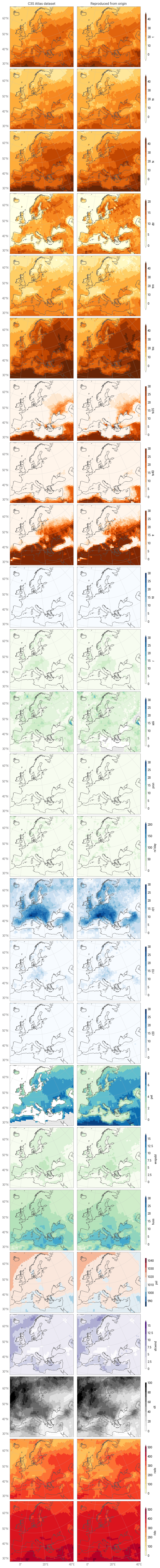
Fig. 7.2.2 Comparison between C3S Atlas dataset and reproduction for multiple indicators in one month, across Europe, on the native grid of each dataset.

Overall comparison

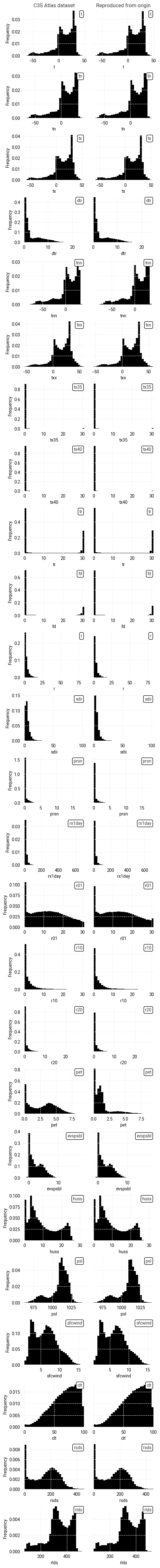
Fig. 7.2.3 Comparison between overall distributions of indicator values in the C3S Atlas dataset and its reproduction, across all spatial and temporal dimensions, on the native grid of each dataset.

Reproducibility: Comparison on C3S Atlas grid

After regridding to the C3S Atlas grid, the indicator values reproduced from the origin dataset can be compared point-by-point to the values retrieved from the C3S Atlas dataset. We first examine some metrics that describe the difference Δ between corresponding pixels:

Show code cell source

Hide code cell source

display_difference_stats(indicators_c3s_atlas_monthly, indicators_cmip6_monthly_regridded, indicators_monthly_names,
                         indicators_relative=indicators_monthly_relative)

C3S Atlas – Reproduced

	Mean Δ	Median Δ	Median |Δ|	% where |Δ| ≥ ε	Median |Δ| [%]	% where |Δ| ≥ 0.1%	Pearson r
t	0.00000	0.00000	0.00028	98.08282	nan	nan	1.00000
tn	-0.00000	0.00000	0.00028	98.08783	nan	nan	1.00000
tx	-0.00000	0.00000	0.00028	98.10905	nan	nan	1.00000
dtr	0.00000	0.00000	0.00033	98.39982	0.01457	6.62924	1.00000
tnn	-0.00000	-0.00000	0.00116	99.52688	nan	nan	1.00000
txx	0.00000	0.00000	0.00116	99.53447	nan	nan	1.00000
tx35	-0.00095	0.00000	0.00000	0.09388	0.00000	0.09079	0.99998
tx40	-0.00047	0.00000	0.00000	0.04720	0.00000	0.04398	0.99998
tr	-0.00216	0.00000	0.00000	12.46425	0.00000	1.12269	1.00000
fd	-0.10867	0.00000	0.00000	18.00463	0.00000	16.25874	0.99978
r	-0.00003	-0.00003	0.00028	98.00682	0.01431	12.93596	1.00000
sdii	-0.00716	-0.00007	0.00042	87.06713	0.00746	8.82253	0.99991
prsn	-0.00000	-0.00000	0.00000	37.15265	0.00000	10.82870	1.00000
rx1day	-0.00000	-0.00001	0.00116	99.49743	0.00997	10.05993	1.00000
r01	0.41235	0.39551	0.40234	86.51813	3.02010	85.46824	0.99926
r10	0.26182	0.04492	0.04590	52.45988	1.34875	52.32150	0.99599
r20	0.14342	0.00000	0.00000	29.29900	0.00000	29.26363	0.98461
pet	-0.04330	-0.00001	0.00025	19.53099	0.00862	2.58153	0.98785
evspsbl	0.00000	0.00000	0.00024	97.97724	0.00839	8.67323	1.00000
huss	0.00013	0.00000	0.00027	98.09658	0.00311	11.36677	1.00000
psl	-0.00003	0.00000	0.00061	96.88182	0.00006	0.00000	1.00000
sfcwind	-0.00000	-0.00000	0.00024	97.95782	0.00392	0.00000	1.00000
clt	0.00000	0.00000	0.00024	97.81430	0.00037	0.05350	1.00000
rsds	0.00000	0.00000	0.00023	92.04655	0.00013	1.08320	1.00000
rlds	0.00000	0.00000	0.00024	97.09195	0.00007	0.00000	1.00000

As in the case study for tx35, it is clear that the C3S Atlas dataset and its manual reproduction are very similar. The median difference, median absolute difference, and median absolute percentage difference are all close to 0 for almost all indicators.

The percentage of pixels with a non-zero difference (defined here as |Δ| ≥ ε with ε = 10^–5 to avoid floating-point errors) is a less useful metric here since most of the indicators are real numbers, rather than integers like tx35. This leaves more room for small differences in the data to appear due to small changes in the origin dataset and/or the C3S Atlas workflow software, which for an integer indicator like tx35 would tend to be rounded off. For most indicators, the relative difference between datasets is ≤0.1% for the vast majority of point-by-point comparisons.

The distributions of indicator values and differences (Figure 7.2.5) confirm that the differences between the two datasets tend to be very small, with distributions centered around 0 and few outliers.

It is not clear why some indicators show larger differences. For pet, the differences are due to masking in a specific region (Northern Fennoscandia; Figure 7.2.4), as discussed before. However, the same is not true for the daily precipitation indicators r01, r10, and r20. These particular indicators show high values and significant spread across Europe in June (and presumably in other months) meaning the differences may simply be due to regridding. This also explains why there are non-integer differences: since the C3S Atlas workflow calculates indicators and then regrids, the regridded indicators can have non-integer values. Similar effects can be seen in other indicators when converting between integer and floating-point data types.

We can extend the conclusion from the tx35 case study, namely that the C3S Atlas dataset can be considered practically reproducible. However, some of the indicators show non-zero differences, either in specific locations (e.g. pet) or distributed randomly (e.g. r01). These differences are caused either by deliberate decisions to mask certain regions or (likely) by small differences in the data processing. They are small and rare enough to be negligible for most users using the C3S Atlas dataset, especially since they will typically use it through the application. For further analysis, it is generally best to manually process the origin dataset, if only to remove the amount of steps that may affect the result.

Show code cell source

Hide code cell source

# Geospatial plot: Monthly indicators
geospatial_comparison_multiple_indicators_with_difference(indicators_c3s_atlas_monthly, indicators_cmip6_monthly_regridded, indicators_monthly_names, month, domain=domain,
                                                          glue_label="derived_multi-origin-c3s-atlas_consistency_q02_fig-geocomp-regional")

Show code cell source

Hide code cell source

# Histogram: Monthly indicators
fig_hist = histogram_comparison_by_indicator_with_difference(indicators_c3s_atlas_monthly, indicators_cmip6_monthly_regridded, indicators_monthly_names,
                                                             indicators_relative=indicators_monthly_relative,
                                                             glue_label="derived_multi-origin-c3s-atlas_consistency_q02_fig-hist-c3s-atlas")

Geospatial comparison

Fig. 7.2.4 Comparison between C3S Atlas dataset and reproduction for multiple indicators in one month, across Europe, on the C3S Atlas dataset grid, including the per-pixel difference.

Overall comparison

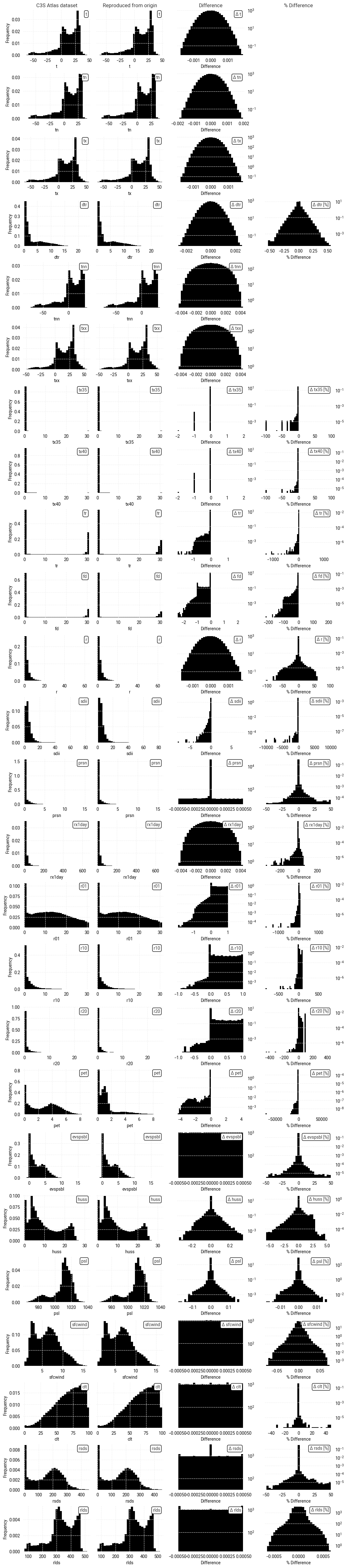
Fig. 7.2.5 Comparison between overall distributions of indicator values in the C3S Atlas dataset and its reproduction on the C3S Atlas grid, across all spatial and temporal dimensions, including the per-pixel difference.

ℹ️ If you want to know more

Key resources

The CDS catalogue entries for the data used were:

• Gridded dataset underpinning the Copernicus Interactive Climate Atlas: multi-origin-c3s-atlas

  • Consistency between the C3S Atlas dataset and its origins: Case study

  • Consistency between the C3S Atlas dataset and its origins: Multiple indicators

  • Consistency between the C3S Atlas dataset and its origins: Multiple origin datasets

• CMIP6 climate projections: projections-cmip6

  • Quality assessments for CMIP6

Code libraries used:

• earthkit

  • earthkit-data

  • earthkit-plots

• User-tools for the C3S Atlas

• xclim climate indicator tools

More about the Copernicus Interactive Climate Atlas and its IPCC predecessor:

• Copernicus Interactive Climate Atlas application

• Gridded data underpinning the Copernicus Interactive Climate Atlas: Description of the datasets and variables

• The Copernicus Interactive Climate Atlas: a tool to explore regional climate change

• Copernicus Interactive Climate Atlas: a new tool to visualise climate variability and change

• Implementation of FAIR principles in the IPCC: the WGI AR6 Atlas repository

• Climate Change 2021 – The Physical Science Basis: Atlas

References

[Gutiérrez+24] J. M. Gutiérrez et al., ‘The Copernicus Interactive Climate Atlas: a tool to explore regional climate change’, ECMWF Newsletter, vol. 181, pp. 38–45, Oct. 2024, doi: 10.21957/ah52ufc369.

[C3S Atlas dataset] Copernicus Climate Change Service, ‘Gridded dataset underpinning the Copernicus Interactive Climate Atlas’. Copernicus Climate Change Service (C3S) Climate Data Store (CDS), Jun. 17, 2024. doi: 10.24381/cds.h35hb680.

[CMIP6 dataset] Copernicus Climate Change Service, ‘CMIP6 climate projections’. Copernicus Climate Change Service (C3S) Climate Data Store (CDS), Mar. 23, 2021. doi: 10.24381/cds.c866074c.

[Burggraaff+20] O. Burggraaff, ‘Biases from incorrect reflectance convolution’, Optics Express, vol. 28, no. 9, pp. 13801–13816, Apr. 2020, doi: 10.1364/OE.391470.