Antarctic Ozone Hole Monitoring Tutorial¶

This tutorial provides guided examples of ozone monitoring using data from the Copernicus Atmosphere Monitoring Service (CAMS). It is divided into two parts:

View animation of Antarctic ozone hole
Calculate the size of the Antarctic ozone hole

It uses CAMS global reanalysis (EAC4) data freely available from the Atmosphere Data Store (ADS)

Run the tutorial via free cloud platforms:

Install and import packages¶

!pip install cdsapi

Requirement already satisfied: cdsapi in c:\users\cxcs\anaconda3\lib\site-packages (0.5.1)
Requirement already satisfied: tqdm in c:\users\cxcs\anaconda3\lib\site-packages (from cdsapi) (4.62.3)
Requirement already satisfied: requests>=2.5.0 in c:\users\cxcs\anaconda3\lib\site-packages (from cdsapi) (2.26.0)
Requirement already satisfied: charset-normalizer~=2.0.0 in c:\users\cxcs\anaconda3\lib\site-packages (from requests>=2.5.0->cdsapi) (2.0.4)
Requirement already satisfied: idna<4,>=2.5 in c:\users\cxcs\anaconda3\lib\site-packages (from requests>=2.5.0->cdsapi) (3.2)
Requirement already satisfied: certifi>=2017.4.17 in c:\users\cxcs\anaconda3\lib\site-packages (from requests>=2.5.0->cdsapi) (2021.10.8)
Requirement already satisfied: urllib3<1.27,>=1.21.1 in c:\users\cxcs\anaconda3\lib\site-packages (from requests>=2.5.0->cdsapi) (1.26.7)
Requirement already satisfied: colorama in c:\users\cxcs\anaconda3\lib\site-packages (from tqdm->cdsapi) (0.4.4)

# CDS API
import cdsapi

# Libraries for reading and working with multidimensional arrays
import numpy as np
import xarray as xr

# Libraries for plotting and animating data
%matplotlib inline
import matplotlib.pyplot as plt
from matplotlib import colors
import matplotlib.animation as animation
import cartopy.crs as ccrs
from IPython.display import HTML

# Disable warnings for data download via API
import urllib3 
urllib3.disable_warnings()

from collections import OrderedDict

View Antarctic ozone hole¶

Let us now visualise our data in form of maps and animations.

We will first define the colour scale we would like to represent our data.

Define colour scale¶

Extract range of values

tco3max = tco3.max()
tco3min = tco3.min()
tco3range = (tco3max - tco3min)/20.

Define colourmap

cmap = plt.cm.jet
norm = colors.BoundaryNorm(np.arange(tco3min, tco3max, tco3range), cmap.N)

Plot map¶

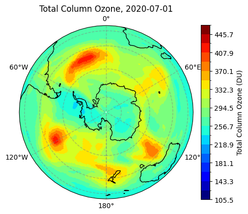
We will now plot our data. Let us begin with a map for the first time step, 1 July 2020.

fig = plt.figure(figsize=(5, 5)) 
ax = plt.subplot(1,1,1, projection=ccrs.Orthographic(central_latitude=-90)) 
ax.coastlines(color='black') # Add coastlines
ax.gridlines(draw_labels=True, linewidth=1, color='gray', alpha=0.5, linestyle='--') 
ax.set_title(f'Total Column Ozone, {str(tco3.time[0].values)[:-19]}', fontsize=12) 
im = plt.pcolormesh(tco3.longitude.values, tco3.latitude.values, tco3[0,:,:],
                cmap=cmap, norm=norm, transform=ccrs.PlateCarree())
cbar = plt.colorbar(im,fraction=0.046, pad=0.04) 
cbar.set_label('Total Column Ozone (DU)') 

Create animation¶

Let us now view the entire time series by means of an animation that shows all time steps. We see from the dataset description above, that the time dimension in our data includes 215 entries. These correspond to 215 time steps, i.e. 215 days, between 1 July 2020 and 31 January 2021. The number of frames of our animation is therefore 215.

frames = 215

Now we will create an animation. The last cell, which creates the animation in Javascript, may take a few minutes to run.

def animate(i):
    array = tco3[i,:,:].values
    im.set_array(array.flatten())
    ax.set_title(f'Total Column Ozone, {str(tco3.time[i].values)[:-19]}', fontsize=12)

ani = animation.FuncAnimation(fig, animate, frames, interval=100)
ani.save(f'{DATADIR}/TCO3_202007-202101_SHem.gif')
HTML(ani.to_jshtml())

2022-09-04 23:27:35,654 INFO Animation.save using <class 'matplotlib.animation.FFMpegWriter'>
2022-09-04 23:27:35,655 INFO MovieWriter._run: running command: ffmpeg -f rawvideo -vcodec rawvideo -s 360x360 -pix_fmt rgba -r 10.0 -loglevel error -i pipe: -filter_complex 'split [a][b];[a] palettegen [p];[b][p] paletteuse' -y .//TCO3_202007-202101_SHem.gif
2022-09-04 23:28:36,187 INFO Animation.save using <class 'matplotlib.animation.HTMLWriter'>

ACTIVITY:
In what date range does the ozone hole appear greatest? In the next section we will quantify the size of the ozone hole at each time step.

Calculate size of ozone hole¶

In this section we will calculate the actual size of the ozone hole, and plot its evolution over our time series. We will then apply the exact same method on monthly averaged data over the past decades to compare ozone hole extents at each yearly occurence since 2003.

Define constants¶

In order to calculate the size of the ozone hole, we need to define some constants. These include the following:

Ozone hole limit, i.e. minimum ozone, in Dobson units, beneath which we consider there to be a hole in the ozone layer.

OZONE_HOLE_LIMIT = 220.

Radius of the Earth, in order to calculate the size of each geographic grid cell of our data.

Rearth = 6371009.

Calculate area of each geographic grid cell of our data¶

Here we calculate the size of each grid cell of our data, which varies as a function of latitude. The formula we apply is the following:

area = |(sin(top latitude) - sin(bottom latitude))| * |Δlongitude| * Earth radius squared

First we define a function to apply this formula, taking as arguments the min and max of the latitudes and longitudes represented by each grid cell:

def geo_area_array(lats1,lons1,lats2,lons2):
    area= np.abs(np.sin(np.deg2rad(lats1)) - np.sin(np.deg2rad(lats2))) * np.abs(np.deg2rad(lons1-lons2))
    area = area * Rearth * Rearth 
    return area

Then we apply this function to our data, defining first the longitude and latitude delta at each grid cell.

DeltaLat = 0.75 # Latitudinal spatial resolution, in degrees
DeltaLon = 0.75 # Longitudinal spatial resolution, in degrees

tco3['areas'] = geo_area_array(tco3['latitude']-DeltaLat/2, tco3['longitude']-DeltaLat/2, 
                             tco3['latitude']+DeltaLat/2, tco3['longitude']+DeltaLat/2)

Mask data belonging to Antarctic ozone hole¶

We now calculate the grid cells that meet the criteria of belonging to the Antarctic ozone hole: i.e. they have less than the minimum threshold of ozone, and they are below -60 degrees latitude.

Here we define a mask with the threshold conditions for ozone and latitude:

mask = tco3.where((tco3 < OZONE_HOLE_LIMIT) & (tco3["latitude"] < -60.))

All data points that do not meet the conditions are set to NaN (Not a Number) in the resulting array. Dividing this array by itself gives us a mask with each valid data point set to 1. Multiplying this by the corresponding areas leaves us with an array of grid cell areas that meet the conditions of belonging to the Antarctic ozone hole.

area = (mask / mask) * mask['areas']

Calculate ozone hole area¶

If we now sum these grid cell areas, we have the total ozone hole extent. This is applied across each time step. We multiply by the number 1e-12 to convert from meters squared to million kilometers squared.

ozone_hole = area.sum(dim=["latitude", "longitude"], skipna=True) * 1e-12

Let us update the Data Array attributes:

ozone_hole.attrs['long_name'] = 'Ozone hole area'
ozone_hole.attrs['units'] = 'million km^2'

Plot ozone hole area at each time step¶

Finally we can plot the evolution of the ozone hole, in million km squared, throughout the time series.

ozone_hole.plot()

[<matplotlib.lines.Line2D at 0x256c24e8280>]

We can also calculate the maximum extent of the ozone hole:

index = ozone_hole.argmax() # Here we find the index of the maximum value
print('Max extent of O3 hole:', ozone_hole[index].values, 'million km2')

Max extent of O3 hole: 23.757296 million km2

… and find out when this was reached:

print('This was reached on:', ozone_hole[index].time.values)

This was reached on: 2020-09-28T00:00:00.000000000

ACTIVITY:
Now repeat the steps above with the data below (see API request in cell below). See what you find out about the evolution of the ozone hole since 2003!

c.retrieve(
    'cams-global-reanalysis-eac4-monthly',
    {
        'format': 'netcdf',
        'variable': 'total_column_ozone',
        'year': [
            '2003', '2004', '2005',
            '2006', '2007', '2008',
            '2009', '2010', '2011',
            '2012', '2013', '2014',
            '2015', '2016', '2017',
            '2018', '2019', '2020',
            '2021',
        ],
        'month': [
            '01', '02', '03',
            '04', '05', '06',
            '07', '08', '09',
            '10', '11', '12',
        ],
        'product_type': 'monthly_mean',
    },
    f'{DATADIR}/TCO3_monthly_2003-2021.nc')

2022-09-09 15:06:35,205 INFO Welcome to the CDS
2022-09-09 15:06:35,205 INFO Sending request to https://ads.atmosphere.copernicus.eu/api/v2/resources/cams-global-reanalysis-eac4-monthly
2022-09-09 15:06:35,299 INFO Downloading https://download-0001-ads-clone.copernicus-climate.eu/cache-compute-0001/cache/data9/adaptor.mars.internal-1658705398.7657485-1943-2-d0f9ab5f-631f-4408-8063-cf04e6396f84.nc to .//TCO3_monthly_2003-2021.nc (50.3M)
2022-09-09 15:06:42,048 INFO Download rate 7.5M/s                                                                      

Result(content_length=52755016,content_type=application/x-netcdf,location=https://download-0001-ads-clone.copernicus-climate.eu/cache-compute-0001/cache/data9/adaptor.mars.internal-1658705398.7657485-1943-2-d0f9ab5f-631f-4408-8063-cf04e6396f84.nc)

CAMS Training

Antarctic Ozone Hole Monitoring Tutorial

Contents

Antarctic Ozone Hole Monitoring Tutorial¶

Install and import packages¶

Download and read and pre-process ozone data¶

Download data¶

Import and inspect data¶

Unit conversion¶