Profile Plots and Zonal Means¶

This tutorial demonstrates how to visualise Copernicus Atmosphere Monitoring Service (CAMS) data of different atmospheric levels in the form of profile plots and zonal mean plots. The data used in this tutorial includes CO from the Northern Hemisphere during the summer (peak fire season) from 2003 to 2021.

Run the tutorial via free cloud platforms:

Install and import packages¶

!pip install cdsapi

Requirement already satisfied: cdsapi in c:\users\cxcs\anaconda3\lib\site-packages (0.5.1)
Requirement already satisfied: tqdm in c:\users\cxcs\anaconda3\lib\site-packages (from cdsapi) (4.62.3)
Requirement already satisfied: requests>=2.5.0 in c:\users\cxcs\anaconda3\lib\site-packages (from cdsapi) (2.26.0)
Requirement already satisfied: charset-normalizer~=2.0.0 in c:\users\cxcs\anaconda3\lib\site-packages (from requests>=2.5.0->cdsapi) (2.0.4)
Requirement already satisfied: idna<4,>=2.5 in c:\users\cxcs\anaconda3\lib\site-packages (from requests>=2.5.0->cdsapi) (3.2)
Requirement already satisfied: certifi>=2017.4.17 in c:\users\cxcs\anaconda3\lib\site-packages (from requests>=2.5.0->cdsapi) (2021.10.8)
Requirement already satisfied: urllib3<1.27,>=1.21.1 in c:\users\cxcs\anaconda3\lib\site-packages (from requests>=2.5.0->cdsapi) (1.26.7)
Requirement already satisfied: colorama in c:\users\cxcs\anaconda3\lib\site-packages (from tqdm->cdsapi) (0.4.4)

# CDS API
import cdsapi

# Libraries for reading and working with multidimensional arrays
import numpy as np
import xarray as xr

# Libraries for plotting and visualising data
%matplotlib inline
import matplotlib.pyplot as plt

# Disable warnings for data download via API
import urllib3 
urllib3.disable_warnings()

Data access and preprocessing¶

Download CAMS global reanalysis data¶

Copy your API key into the code cell below, replacing ####### with your key. (Remember, to access data from the ADS, you will need first to register/login https://ads.atmosphere.copernicus.eu and obtain an API key from https://ads.atmosphere.copernicus.eu/api-how-to.)

URL = 'https://ads.atmosphere.copernicus.eu/api/v2'

# Replace the hashtags with your key:
KEY = '##########################################'

Here we specify a data directory into which we will download our data and all output files that we will generate:

DATADIR = '.'

For this tutorial, we will use CAMS Global Reanalysis (EAC4) data. The code below shows the subset characteristics that we will extract from this dataset as an API request.

Note

Before running this code, ensure that you have accepted the terms and conditions. This is something you only need to do once for each CAMS dataset. You will find the option to do this by selecting the dataset in the ADS, then scrolling to the end of the Download data tab.

c = cdsapi.Client(url=URL, key=KEY)
c.retrieve(
    'cams-global-reanalysis-eac4-monthly',
    {
        'variable': 'carbon_monoxide',
        'pressure_level': [
            '100', '150', '200',
            '250', '300', '400',
            '500', '600', '700',
            '800', '850', '900',
            '925', '950', '1000',
        ],
        'year': [
            '2003', '2004', '2005',
            '2006', '2007', '2008',
            '2009', '2010', '2011',
            '2012', '2013', '2014',
            '2015', '2016', '2017',
            '2018', '2019', '2020',
            '2021',
        ],
        'month': [
            '06', '07', '08',
        ],
        'product_type': 'monthly_mean',
        'format': 'netcdf',
    },
    f'{DATADIR}/CO_NHemis_JJA_2003-2021.nc')

2022-09-11 12:16:55,355 INFO Welcome to the CDS
2022-09-11 12:16:55,358 INFO Sending request to https://ads.atmosphere.copernicus.eu/api/v2/resources/cams-global-reanalysis-eac4-monthly
2022-09-11 12:16:55,428 INFO Request is queued
2022-09-11 12:16:56,494 INFO Request is running
2022-09-11 12:17:45,252 INFO Request is completed
2022-09-11 12:17:45,253 INFO Downloading https://download-0005-ads-clone.copernicus-climate.eu/cache-compute-0005/cache/data9/adaptor.mars.internal-1662894988.4514306-17529-12-b1ed787e-7c7b-4d76-97a7-540ec28e5ca9.nc to ./CO_NHemis_JJA_2003-2021.nc (188.7M)
2022-09-11 12:18:02,626 INFO Download rate 10.9M/s                                                                     

Result(content_length=197817276,content_type=application/x-netcdf,location=https://download-0005-ads-clone.copernicus-climate.eu/cache-compute-0005/cache/data9/adaptor.mars.internal-1662894988.4514306-17529-12-b1ed787e-7c7b-4d76-97a7-540ec28e5ca9.nc)

Representation of pressure levels¶

Our CO dataset represents 15 levels of the atmosphere, from 1000 (surface) to 100 hectopascals (hPa). This can be best visualised in a logarithmic scale, or if converted to altitude.

Pressure levels in logarithmic scale¶

Here we create a new coordinate of our Data Array with the logarithm of the pressure levels, to facilitate visualisation in our plots.

ds['level_log10'] = np.log10(ds['level'])

ds = ds.set_coords('level_log10')

Pressure levels to altitude¶

Here we create a new coordinate with altitude. The altitude in meters can be calculated with the international barometric formula:

H = 44330 * [1 - (P/p0)^(1/5.255) ]

Where H = altitude (m), P = measured pressure (Pa) from the sensor, and p0 = reference pressure at sea level (e.g. 1000 hPa)

Here we shall assume that the reference pressure at sea level is 1000 hPa.

ds['height'] = 44330. * (1 - ((ds['level']/1000.)**(1/5.255)))

We will convert the heights from meters to kilometers:

ds['height'] = ds['height']/1000.

Here we set the heights as a coordinate in our Xarray Dataset.

ds = ds.set_coords('height')

Unit conversion¶

Most of the chemical species in the CAMS Global data, including our CO data, is archived as mass mixing ratios (MMR, kg of gas / kg of air).

We will convert this to Volume Mixing Ratio (VMR, in units parts per billion, or ppbv)

To convert data from MMR to VMR you only need the molar masses of dry air and of the atmospheric species. For CO the formula is: VMR = 28.9644 / 28.0101 * 1e9 * MMR. The 1e9 in the formulae gives parts per billion (ppbv). If we wanted parts per million (ppmv) we would use 1e6. See more details on unit conversions here.

da = (28.9644 / 28.0101) * 1e9 * da

Here we update the attributes of our dataset with the new units.

da.attrs['long_name'] = 'CO Volume Mixing Ratio'
da.attrs['units'] = 'ppbv'

Subset and aggregation¶

We would like to visualise CO profiles over the northern hemisphere, so we will take a subset including only northern latitudes. Also, to facilitate visualisation of CO vertical profiles, we are going to average over the temporal and spatial dimensions.

Spatial subset¶

Here we subset the data to keep only northern latitudes.

da_north = da.where(da.latitude > 0, drop=True)

Temporal aggregation¶

The purpose of the temporal aggregation is to average June, July and August in each year, resulting in one summer mean value at each year of the dataset.

summer = da_north.groupby('time.year').mean(keep_attrs=True)

Spatial aggregation¶

To visualise the data in a profile plot, we will aggregate over the spatial dimensions. For the latitudinal dimension, we need to take into account the variation in area as a function of latitude, which we will do by taking the cosine of the latitude as a proxy.

weights = np.cos(np.deg2rad(summer.latitude))
weights.name = "weights"
weighted = summer.weighted(weights)

# Average (mean) over the latitudinal axis
co = weighted.mean(dim=["latitude", "longitude"])

Calculate quantiles of climatology¶

Here we calculate the 5th, 50th and 95th quantile of CO climatology from 2003 to 2021.

co95 = co.quantile(0.95, dim='year')
co05 = co.quantile(0.05, dim='year')
co50 = co.quantile(0.5, dim='year')

Plot summer climatology of CO in Northern Hemisphere¶

fig, ax = plt.subplots(1, 1, figsize = (6, 9))

ax.set_title('CO in JJA in Northern Hemisphere', fontsize=12)
ax.set_ylabel('Height [Kilometers]')
ax.set_xlabel('CO [ppbv]')
ax.plot(co50, co50.height, color='black', linestyle='--', label='2003-2021 median')
ax.fill_betweenx(co50.height, co05, co95, alpha=0.1, color='black', label='2003-2021 5th to 95th quantile range')
ax.plot(co[18,:], co.height, color='red', linestyle='-', label='2021')
ax.plot(co[17,:], co.height, color='green', linestyle='-', label='2020')
ax.plot(co[16,:], co.height, color='blue', linestyle='-', label='2019')

handles, labels = ax.get_legend_handles_labels()
ax.legend(handles, labels)

fig.savefig(f'{DATADIR}/CO_JJA_NHem_2003-2021_profile.png')

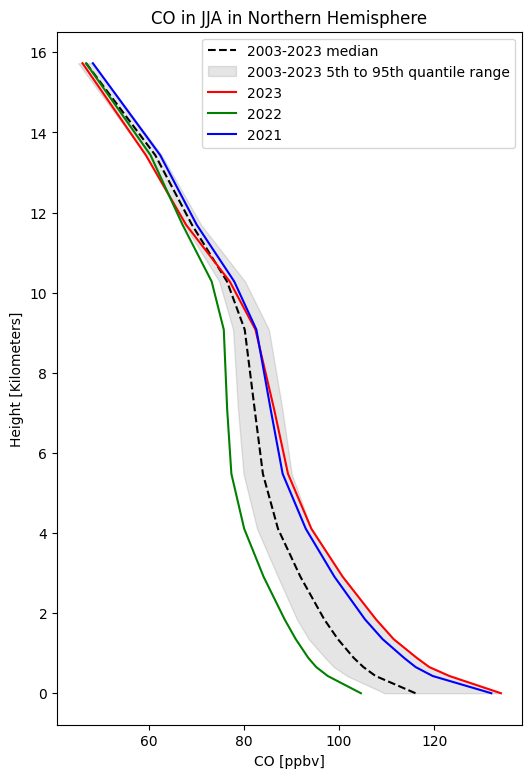
Note the distribution of CO mainly in the lower part of the atmosphere, and the high values in 2021, due mainly to the significant wildfire activity that summer. See the BAMS State of the Climate 2021 report for more details.

Create zonal mean plot of CO summer climatology in Northern Hemisphere¶

Data prep¶

We again aggregate over time (June, July and Aug of each year), and over space. This time however the spatial aggregation is only over the longitudinal dimension, as we want to visualise data over all latitudinal zones.

jja = da.groupby('time.year').mean(keep_attrs=True)

zonal = jja.mean(dim=["longitude", "year"])

Create zonal mean plot¶

Now we can plot our data. Before we do this however, we define the min, max and step of contours that we will use in a contour plot.

vdiv = 10
vmin = 50
vmax = 200+vdiv
clevs = np.arange(vmin,vmax,vdiv)

# Define the figure and specify size
fig, ax = plt.subplots(1, 1, figsize = (9, 6))

# Configure the axes and figure title
ax.set_xlabel('Latitude [degrees]')
ax.set_ylabel('Altitude [km]')
ax.set_title('Zonal mean of CO in N. Hemisphere for JJA climatology (2003 to 2021)', fontsize=12)

# As the altitudes (15) are much less than the latitudes (180),
# we need to ensure the plot fits into the size of the figure.
ax.set_aspect('auto')

# Plot the data as a contour plot
contour = ax.contourf(zonal.latitude, zonal.height, zonal, levels=clevs, cmap='YlOrRd', extend='max')

# Specify the colourbar
cbar = plt.colorbar(contour,fraction=0.046, pad=0.04)
cbar.set_label('CO [ppbv]')

# Save the plot
fig.savefig(f'{DATADIR}/CO_JJA_NHem_2003-2021_zonal_mean.png')

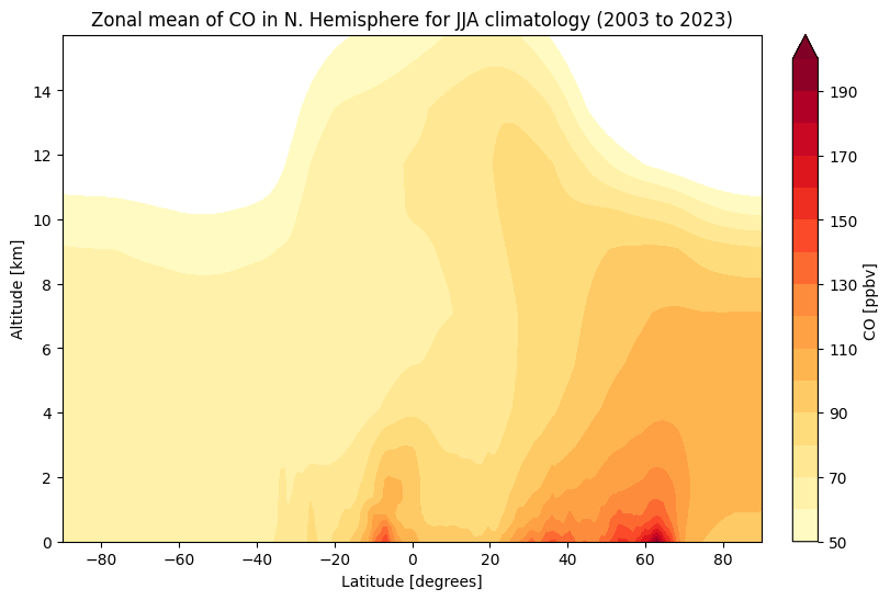
Note the greater abundance of CO in the northern hemisphere, and in the lower part of the atmosphere.

CAMS Training

Profile Plots and Zonal Means

Contents