
Visualising a full Climate Data Record of multi-sensor Aerosol data#
This second notebook extends the practical introduction of the first notebook to the C3S Aerosol properties gridded data from 1995 to present derived from satellite observations dataset.
Now, we create a full Climate Data Record from 1995 to 2023. This can only be achieved by combining shorter data record pieces from subsequent similar sensors.
We start by downloading the data from the Climate Data Store (CDS) and then demonstrate three use cases for monthly mean multi-sensor data records: calculate and plot a regional data record, calculate and plot a regional multi-annual mean (“climatology”) and plot a regional anomaly time series.
The notebook has six main sections with the following outline:
Table of Contents#
How to access the notebook#
This tutorial is in the form of a Jupyter notebook. You will not need to install any software for the training as there are a number of free cloud-based services to create, edit, run and export Jupyter notebooks such as this. Here are some suggestions (simply click on one of the links below to run the notebook):
Binder |
Kaggle |
Colab |
NBViewer |
|---|---|---|---|
|
|
|
|
(Binder may take some time to load, so please be patient!) |
(will need to login/register, and switch on the internet via settings) |
(will need to run the command |
(this will not run the notebook, only render it) |

If you would like to run this notebook in your own environment, we suggest you install Anaconda, which contains most of the libraries you will need. You will also need to install the CDS API (pip install cdsapi) for downloading data in batch mode from the CDS.
Introduction#
This second notebook focuses on combining subsequent parts of a long term record from a sequence of similar sensors, so that a relevant Climate Data Record (covering at least three decades) can be provided.
We combine now three AOD data records from three similar dual-view radiometers ATSR-2 (Along Track Scanning Radiometer no. 2), AATSR (Advanced ATSR) and SLSTR (Sea and Land Surface Temperature Radiometer). This can be done since all three instruments use the same measurement principle (conical scan which enables observing the Earth surface with two viewing directions: nadir and oblique) and have the same set of seven visual and infrared channels. However, there are remaining differences between the instruments in data rates / sampling and most importantly, the pointing direction of the oblique view (forward for ATSR-2 and AATSR, rearward for SLSTR).
A user should be aware that slower long-term changes of atmospheric aerosols can only be seen in records of several decades while exceptionally large episodic extreme events may be visible in short records of a few years only.
Data description#
The data are provided in netCDF format.
Please find further information about the dataset as well as the data in the Climate Data Store catalogue entry Aerosol properties, sections “Overview”, “Download data” and “Documentation”:
There in the “Documentation” part, one can find the Product User Guide and Specifications (PUGS) and the Algorithm Theoretical Baseline (ATBD) for further information on the different algorithms.
Import libraries#
We will be working with data in NetCDF format.
To best handle this data we will use the netCDF4 python library. We will also need libraries for plotting and viewing data, in this case we will use Matplotlib and Cartopy.
We are using cdsapi to download the data. This package is not yet included by default on most cloud platforms. You can use pip to install it:
#!pip install cdsapi
%matplotlib inline

# CDS API library
import cdsapi

# Libraries for working with multidimensional arrays
import numpy as np
import numpy.ma as ma
import netCDF4 as nc

# Library to work with zip-archives, OS-functions and pattern expansion
import zipfile
import os
from pathlib import Path

# Libraries for plotting and visualising data
import matplotlib.pyplot as plt
import matplotlib as mplt
import matplotlib.dates as md
import cartopy.crs as ccrs

# Libraries for style parameters
from pylab import rcParams

# Disable warnings for data download via API
import urllib3
urllib3.disable_warnings()
# The following style parameters will be used for all plots in this use case.
mplt.style.use('seaborn')
rcParams['figure.figsize'] = [15, 5]
rcParams['figure.dpi'] = 350
rcParams['font.family'] =  'serif'
rcParams['font.serif']  =  mplt.rcParamsDefault['font.serif']
rcParams['mathtext.default'] = 'regular'
rcParams['mathtext.rm'] = 'serif:light'
rcParams['mathtext.it'] = 'serif:italic'
rcParams['mathtext.bf'] = 'serif:bold'
plt.rc('font', size=17)          # controls default text sizes
plt.rc('axes', titlesize=17)     # fontsize of the axes title
plt.rc('axes', labelsize=17)     # fontsize of the x and y labels
plt.rc('xtick', labelsize=15)    # fontsize of the tick labels
plt.rc('ytick', labelsize=15)    # fontsize of the tick labels
plt.rc('legend', fontsize=10)    # legend fontsize
plt.rc('figure', titlesize=18)   # fontsize of the figure title

projection=ccrs.PlateCarree()
mplt.rc('xtick', labelsize=9)
mplt.rc('ytick', labelsize=9)
/tmp/ipykernel_1983506/2007949843.py:2: MatplotlibDeprecationWarning: The seaborn styles shipped by Matplotlib are deprecated since 3.6, as they no longer correspond to the styles shipped by seaborn. However, they will remain available as 'seaborn-v0_8-<style>'. Alternatively, directly use the seaborn API instead.
  mplt.style.use('seaborn')
Download data using CDS API#
CDS API credentials#
We will request data from the CDS in batch mode with the help of the CDS API.
First, we need to manually set the CDS API credentials.
To do so, we need to define two variables: URL and KEY.
To obtain these, first login to the CDS, then visit https://cds.climate.copernicus.eu/api-how-to and copy the string of characters listed after “key:”. Replace the ######### below with this string.
URL = 'https://cds.climate.copernicus.eu/api/v2'
# KEY = 'XXXXXXXXXXXXXXXXXXXXXXXXXXXXXXXXXXXXXXXXX'
Next, we specify a data directory in which we will download our data and all output files that we will generate:
DATADIR='./test_long/'
if not os.path.exists(DATADIR):
    os.mkdir(DATADIR)
Long Time Series#
To start, we need to define the variable, algorithm and region for our analysis. Furthermore, latest dataset versions for each Dual view algorithm are specified.
variable = 'aerosol_optical_depth'
algorithm = 'SWANSEA'
region = 'Europe'
years = ['%04d'%(yea) for yea in range(1995, 2023)]
version_ATSR2 = {'ORAC': 'v4.02',
                'ADV': 'v2.30',
                'SWANSEA': 'v4.33',
                'ENS': 'v2.9',}
version_AATSR = {'ORAC': 'v4.02',
                'ADV': 'v3.11',
                'SWANSEA': 'v4.33',
                'ENS': 'v2.9',}
version_SLSTR = {'ORAC': 'v1.00',
                'SDV': 'v2.00',
                'SWANSEA': 'v1.12',
                'ENS': 'v1.1',}
Next, we implement definitions of some relevant regions, define the temporal coverage for each instrument in the sensor series and extract cell indices for the selected region.
extent = { # 'Region' : [lon_min, lon_max, lat_min, lat_max],
            'Europe': [-15, 50, 36, 60],
            'Boreal': [-180, 180, 60, 85],
            'Asia_North': [50, 165, 40, 60],
            'Asia_East': [100, 130, 5, 41],
            'Asia_West': [50, 100, 5, 41],
            'China_South-East': [103, 135, 20, 41],
            'Australia': [100, 155, -45, -10],
            'Africa_North': [-17, 50, 12, 36],
            'Africa_South': [-17, 50, -35, -12],
            'South_America': [-82, -35, -55, 5],
            'North_America_West': [-135, -100, 13, 60],
            'North_America_East': [-100, -55, 13, 60],
            'Indonesia': [90, 165, -10, 5],
            'Atlanti_Ocean_dust': [-47, -17, 5, 30],
            'Atlantic_Ocean_biomass_burnig': [-17, 9, -30, 5],
            'World': [-180, 180, -90, 90],
            'Asia': [50, 165, 5, 60],
            'North_America': [-135, -55, 13, 60],
            'dust_belt': [-80, 120, 0, 40],
            'India': [70, 90, 8, 32],
            'Northern_Hemisphere': [-180, 180, 0, 90],
            'Southern_Hemisphere': [-180, 180, -90, 0],
            }
years_ATSR2 = ['1995', '1996', '1997', '1998', '1999', '2000', '2001', '2002']
years_AATSR = ['2003', '2004', '2005', '2006', '2007', '2008', '2009', '2010', '2011']
years_SLSTR = ['2017', '2018', '2019', '2020', '2021', '2022']
years_dual = years_ATSR2 + years_AATSR + years_SLSTR
months = ['%02d'%(mnth) for mnth in range(1,13)]
area_coor = extent[region]
# calculate Cell indices out of coordinates
lon1 = 180 + area_coor[0]
lon2 = 180 + area_coor[1]
lat1 = 90 + area_coor[2]
lat2 = 90 + area_coor[3]
Download data using CDS API#
Then we prepare and start the CDS download.
To search for data, visit the CDS website: https://cds.climate.copernicus.eu/cdsapp#!/home. Here you can search for aerosol data using the search bar. The data we need for this use case is the C3S Aerosol properties gridded data from 1995 to present derived from satellite observations.
c = cdsapi.Client(url=URL, key=KEY)
product='satellite-aerosol-properties'
We now download the full time record of one dual view algorithm 1995 - 2022: The following download may take ~ 15 min (exact time needed depends on your network and hardware). Do not worry, as there may be many error messages for missing months in gaps.
for year in years:
    if year in years_ATSR2:
        Instrument = 'atsr2_on_ers2'
        if algorithm == 'ADV/SDV':
            algorithm = 'ADV'
        version = version_ATSR2[algorithm]
    elif year in years_AATSR:
        Instrument = 'aatsr_on_envisat'
        if algorithm == 'ADV/SDV':
            algorithm = 'ADV'
        version = version_AATSR[algorithm]
    elif year in years_SLSTR:
        Instrument = 'slstr_on_sentinel_3a'
        if algorithm == 'ENS':
            if year == '2019':
                version = 'v1.2'
            else:
                version = version_SLSTR[algorithm]
        elif algorithm == 'ADV/SDV' or algorithm == 'ADV':
            algorithm = 'SDV'
            if year == '2017':
                version = 'v1.10'
            else:
                version = version_SLSTR[algorithm]
        else:
            version = version_SLSTR[algorithm]

    for month in months:
        if year in years_dual:
            try:
                request = {
                        'time_aggregation': 'monthly_average',
                        'variable': variable,
                        'sensor_on_satellite': Instrument,
                        'algorithm': algorithm.lower(),
                        'year': year,
                        'month': month,
                        'version': version}
                file_name = DATADIR + algorithm + '_' + str(year) + '_' + str(month) + '.zip'
                c.retrieve(product, request, file_name)
            except:
                print('no data' + year + month)
Next, we unpack the data.
files = os.listdir(DATADIR)
dir = f'{DATADIR}' + 'data/'

for file in files:
    if '.zip' in file:
        with zipfile.ZipFile(DATADIR + file, 'r') as zip_ref:
            zip_ref.extractall(f'{DATADIR}' + 'data')
        os.remove(DATADIR + file)

files = os.listdir(dir)
Correction of variable names: There are a few variable naming inconsistencies which we automatically adjust by the following code block.
Those inconsistencies are remaining despite of strong format harmonization efforts from the fact that the algorithms / datasets come from different providers who have somewhat different coding practices.
if variable == 'aerosol_optical_depth':
    if algorithm == 'ens':
        variable = 'AOD550'
    else:
        variable = 'AOD550_mean'
elif variable == 'fine_mode_aerosol_optical_depth':
    if algorithm == 'ens':
        variable = 'FM_AOD550'
    else:
        variable = 'FM_AOD550_mean'
elif variable == 'dust_aerosol_optical_depth':
    if algorithm == 'ens':
        variable = 'DAOD550'
    elif algorithm == 'lmd':
        variable = 'Daod550'
    elif algorithm == 'imars':
        variable = 'D_AOD550'
    else:
        variable = 'D_AOD550_mean'
Use case 1: extract and plot long time series#
Finally, we get the regional time series as list.
Since the validation showed a significant bias for SLSTR algorithms with some but limited regional variations, we have to subtract it before combining the time series. Note that we use a global average bias here, while a more sophisticated correction will use regional biases. The bias correctino was detemring by comparison to AOD data from the global sun photometer network AERONET.
if algorithm == 'SWANSEA':
    slstr_bias = 0.045
if algorithm == 'ORAC':
    slstr_bias = 0.06
if algorithm == 'SDV':
    slstr_bias = 0.07
if algorithm == 'ENS':
    slstr_bias = 0.03

aod = []
time = []

for year in years_dual:
    for month in months:
        t_str = year + '-' + month
        t = year + month
        len1 = len(aod)
        time.append(md.datestr2num(t_str))
        try:
            for file in files:
                if t in file:
                    correct = 0
                    if file[35:40] == 'SLSTR':
                        correct = slstr_bias
                    data_set = nc.Dataset(dir + file,'r')
                    data_sel = data_set[variable][lat1 : lat2 , lon1 : lon2]
                    data_mean = np.ma.mean(data_sel) - correct
                    aod.append(data_mean)
                    data_set.close()
        except:
            aod.append(np.nan)
        if len1 == len(aod):
            aod.append(np.nan)
Here, we plot the long time series.
plt.plot_date(time, aod, '-', label = variable, linewidth = 0.5)
plt.ylabel("AOD")
plt.title(variable + ' Timeseries ' + algorithm + ' in ' + region)
plt.savefig(DATADIR + 'timeseries_' + variable + '_' + algorithm + '_' + region + '.png', dpi=500, bbox_inches='tight')
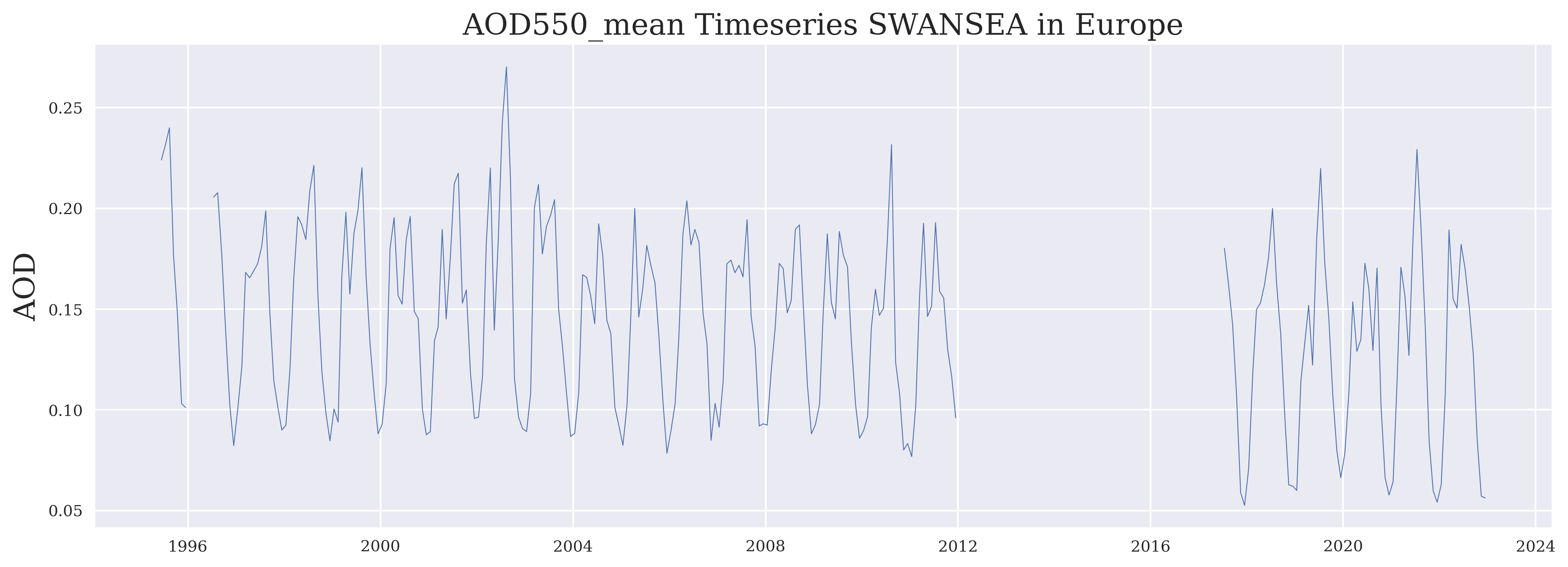
FIGURE 1: This time series shows the long term behaviour of aerosol properties in the selected region. Note that a global bias correction was applied for the last part (SLSTR) which may be a bit too large for this region.
Use case 2: Calculate and plot a multi-annual mean (“climatology”)#
We calculate a multi-annual mean for each sensor in the time series, i.e. for ATSR-2 (1995-2002), AATSR (2003-2011) and SLSTR (2017-2022) and use each of them for the respective time series. We calcualte the multi-annual means separately per sensor, sicne there is no overlap between AATSR and SLSTR which would allow a relative bias correction without extrapolation.
## Climatology
aod_standard_deviation_ges = []
aod_climatology_ges = []
#ATSR2
aod_standard_deviation1 = []
aod_climatology1 = []
for month in months:
    aodmonth1 = []
    aodvar1 = []
    for year in years_ATSR2[2:]:
        t = year + month
        for file in files:
            if t in file:
                data_set = nc.Dataset(dir + file,'r')
                data_sel = data_set[variable][lat1 : lat2 , lon1 : lon2]
                data_mean = np.ma.mean(data_sel)
                data_var = (data_mean**2)/len(years_ATSR2[2:])
                aodmonth1.append(data_mean)
                aodvar1.append(data_var)
    expectation = sum(aodmonth1)/len(years_ATSR2[2:])
    standard_deviation = np.sqrt(sum(aodvar1)-expectation**2)
    aod_climatology1.append(expectation)
    aod_standard_deviation1.append(standard_deviation)

for i in range(len(years_ATSR2)):
    aod_climatology_ges.extend(aod_climatology1)
    aod_standard_deviation_ges.extend(aod_standard_deviation1)

#AATSR
aod_standard_deviation1 = []
aod_climatology1 = []
for month in months:
    aodmonth1 = []
    aodvar1 = []
    for year in years_AATSR:
        t = year + month
        for file in files:
            if t in file:
                data_set = nc.Dataset(dir + file,'r')
                data_sel = data_set[variable][lat1 : lat2 , lon1 : lon2]
                data_mean = np.ma.mean(data_sel)
                data_var = (data_mean**2)/len(years_AATSR)
                aodmonth1.append(data_mean)
                aodvar1.append(data_var)
    expectation = sum(aodmonth1)/len(years_AATSR)
    standard_deviation = np.sqrt(sum(aodvar1)-expectation**2)
    aod_climatology1.append(expectation)
    aod_standard_deviation1.append(standard_deviation)

for i in range(len(years_AATSR)):
    aod_climatology_ges.extend(aod_climatology1)
    aod_standard_deviation_ges.extend(aod_standard_deviation1)

#DATA GAP
nan_list = [np.nan for i in range(12)]
aod_climatology_ges.extend(nan_list)
aod_standard_deviation_ges.extend(nan_list)
#SLSTR
aod_standard_deviation1 = []
aod_climatology1 = []
for month in months:
    aodmonth1 = []
    aodvar1 = []
    for year in years_SLSTR:
        t = year + month
        for file in files:
            if t in file:
                data_set = nc.Dataset(dir + file,'r')
                data_sel = data_set[variable][lat1 : lat2 , lon1 : lon2]
                data_mean = np.ma.mean(data_sel) - correct
                data_var = (data_mean**2)/len(years_SLSTR)
                aodmonth1.append(data_mean)
                aodvar1.append(data_var)
    expectation = sum(aodmonth1)/len(years_SLSTR)
    standard_deviation = np.sqrt(sum(aodvar1)-expectation**2)
    aod_climatology1.append(expectation)
    aod_standard_deviation1.append(standard_deviation)

for i in range(len(years_SLSTR)):
    aod_climatology_ges.extend(aod_climatology1)
    aod_standard_deviation_ges.extend(aod_standard_deviation1)

aod_standard_deviation1 = [aod_climatology_ges[i] + aod_standard_deviation_ges[i] for i in range(len(aod_standard_deviation_ges))]
aod_standard_deviation2 = [aod_climatology_ges[i] - aod_standard_deviation_ges[i] for i in range(len(aod_standard_deviation_ges))]

years_dual = years_ATSR2 + years_AATSR + ['2016'] + years_SLSTR
time_dual = []
for year in years_dual:
    for month in months:
        t_str = year + '-' + month
        time_dual.append(md.datestr2num(t_str))
Now we plot the time series with the climatologies.
fig = plt.figure(figsize=(7,3))
plt.plot_date(time, aod, '-', label = variable, color = 'red', linewidth = 0.5)
plt.fill_between(time_dual, aod_standard_deviation1, aod_standard_deviation2, color = 'blue', alpha = 0.2)
plt.plot(time_dual, aod_climatology_ges, '-', label = 'climatology', color = 'blue', linewidth = 0.5, alpha = 0.5)
plt.ylabel("AOD")
plt.legend()
plt.title(variable + ' Climatology ' + algorithm + ' in ' + region)
plt.savefig(DATADIR + 'timeseries_with_climatology_' + variable + '_' + algorithm + '_' + region + '.png', dpi=500, bbox_inches='tight')
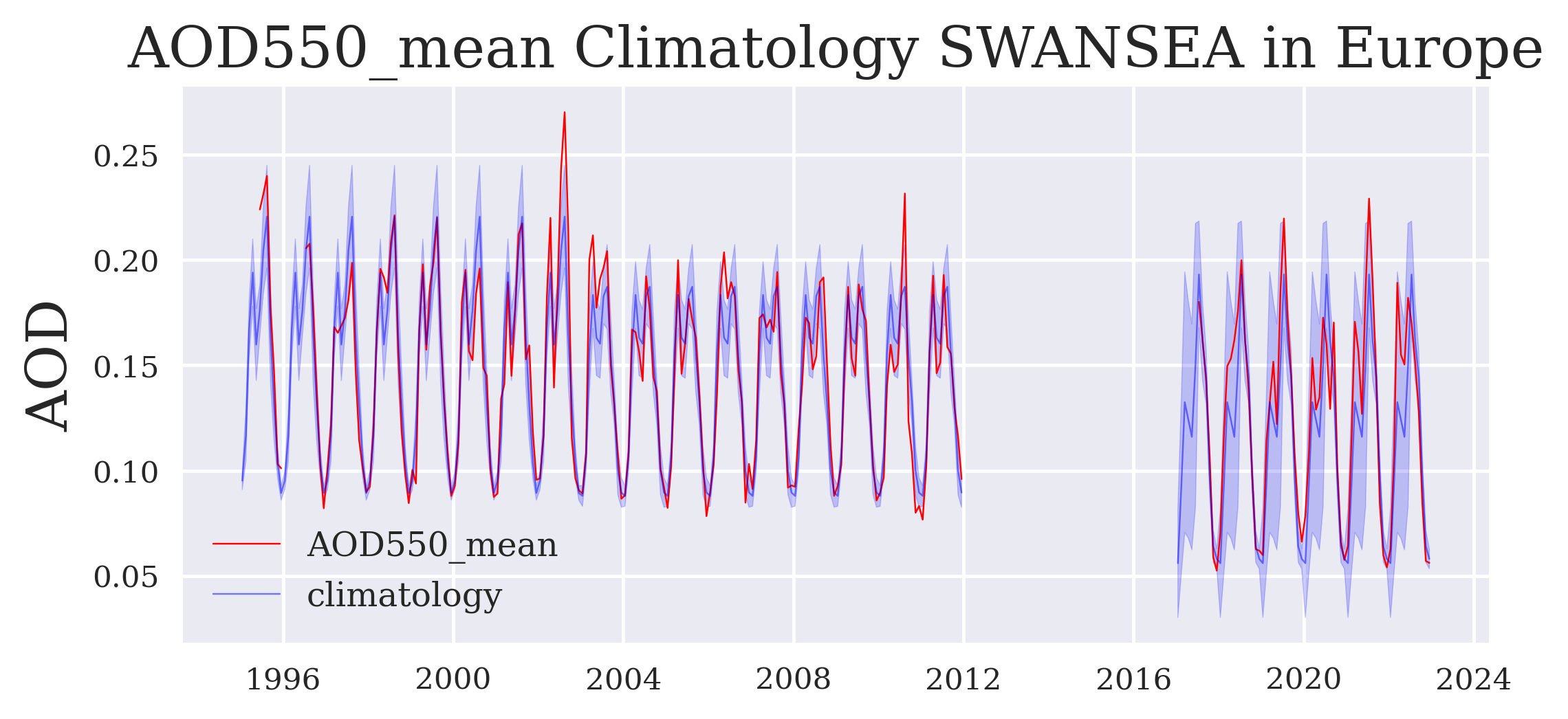
FIGURE 2: This time series plotted over repeated annual climatologies (per sensor) already indicates any episodic events outside the long-term variabiliy. Note that a global bias correction was applied for the last part (SLSTR) which may be a bit too large for this region.
Use case 3: Calculate and plot the anomaly time series#
anomaly = [aod[i] - aod_climatology_ges[i] for i in range(len(aod))]
aod_standard_deviation_ges_ = [-aod_standard_deviation_ges[i] for i in range(len(aod_standard_deviation_ges))]

fig = plt.figure(figsize=(7,3))
plt.plot_date(time, anomaly, '-', label = variable, color = 'red', linewidth = 0.5)
plt.fill_between(time_dual, aod_standard_deviation_ges, aod_standard_deviation_ges_, color = 'blue', alpha = 0.2)
plt.plot(time, anomaly, '-', label = 'climatology', color = 'blue', linewidth = 0.5, alpha = 0.5)
plt.plot(time, anomaly, '-', color = 'red', linewidth = 0.5)
plt.ylabel("AOD")
plt.legend()
plt.title(variable + ' Anomaly ' + algorithm + ' in ' + region)
plt.savefig(DATADIR + 'anomaly_timeseries_' + variable + '_' + algorithm + '_' + region + '.png', dpi=500, bbox_inches='tight')
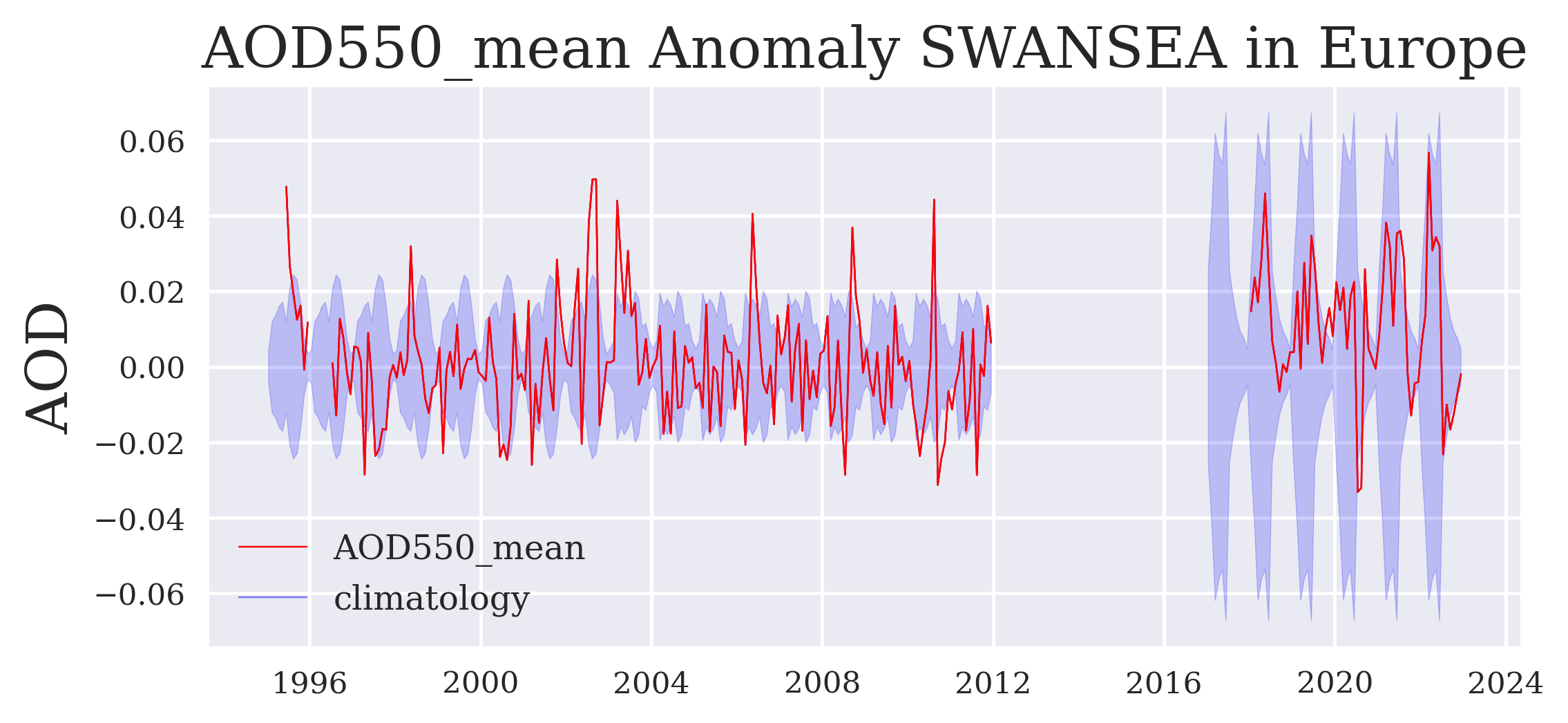
FIGURE 3: This anomaly record shows more clearly those episodic extreme events as outliers outside the shaded long-term variability and possibly also any trend of the data record in this region (e.g. decreases in Europe or the U.S., increases in India or on Sout-Eact China increases before ~2008 and decreases since ~2012).
This closes our second Jupyter notebook on aerosol properties.