

The Total Solar Irradiance (TSI) from RMIB#
This notebook provides a practical introduction to the Total Solar Irradiance (TSI) dataset available at the Copernicus Climate Change Service (C3S) Climate Data Store (CDS).
The notebook begins with an introduction to the TSI variable and the dataset overview. Next, it provides instructions for setting up and running the notebook. It describes the steps to set up a python environment, and access and prepare the data. Following this setup, the notebook presents two practical use cases of the dataset: plotting the TSI daily values and a 12-month rolling mean (Use Case 1), and plotting two TSI datasets side-by-sides (Use Case 2).
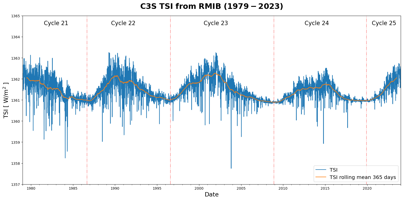
The figure below is the result of Use Case 1, and the result of a successful run of the code.
Table of Contents#
Introduction
Prerequisites and data preparations
Use cases
Use case 1: Time series of the Total Solar Irradiance (TSI)
Use case 2: Comparison of two TSI composites
References
1. Introduction#
The Total Solar Irradiance (TSI) is the measure of the energy input that the Earth receives from the Sun. It is the dominant driver of the Earth’s climate, a key component of the Earth’s Radiation Budget (ERB), and is thus one of the Global Climate Observing System (GCOS) Essential Climate Variables (ECVs). Stable and accurate long-term TSI records are needed for climate studies, e.g. to understand the influence of solar variability on climate.
The TSI exhibits large day-to-day variations due to the passage of dark sunspots, and bright faculae. The well-known 11-year solar cycle is also being directly observed by space-based instruments. There exist other regular and irregular factors that contribute to the short-term variations of TSI. Fortunately, the TSI is very stable in the long timescales, century to multi-century (thus the historical name “the solar constant”, now usually referred to as Total Solar Irradiance (TSI)).
This TSI dataset provides daily TSI observations for over 44 years. It is a composite dataset, meaning that it is constructed from different TSI measurements obtained by an ensemble of space instruments, and carefully combined into one homogeneous dataset.
This dataset is produced on behalf of C3S by the Royal Meteorological Institute of Belgium (RMIB).
Please find further information about the dataset as well as the data in the Climate Data Store catalogue entry Earth’s Radiation Budget, sections “Overview”, “Download data” and “Documentation”:
A tutorial video describes the “Earth Radiation Budget” Essential Climate Variable and the methods and satellite instruments used to produce the data provided in the CDS catalogue entry.
2. Prerequisites and data preparations#
This chapter provides information on how to: run the notebook, lists necessary python libraries, and guides you through the process of the preparation: how to search and download the data via CDS API and get it ready to be used.
2.1 How to access the notebook#
This tutorial is in the form of a Jupyter notebook. This tutorial can also be run on a cloud environment, or on your own computer. Here are some suggestions, simply click on one of the links below to launch this notebook in the cloud environment. To run the code, press “Run - Run All Cells”. Once you feel comfortable with the python code, you are invited to adjust or extend the code according to your interests.
| Run the tutorial via free cloud platforms: |
|
|
|---|
We are using cdsapi to download the data. This package is not yet included by default on most cloud platforms. You can use pip to install it:
!pip install cdsapi
Run the tutorial in the local environment
If you would like to run this notebook in your own environment, download this notebook as an ipynb file. We suggest you install Anaconda or mamba, which contains most of the libraries you will need.
We will be working with data in ASCII format. pandas is a Python library for data manipulation and analysis. It is used to read, process, and write ASCII files such as TXT or CSV. We will also need libraries for plotting and viewing data, in this case, we will use Matplotlib. cdsapi is a Python library for programmatically accessing the data from the CDS.
2.2 Import libraries#
We need to import the libraries to ensure that all necessary functions and modules are available for use throughout the script’s execution.
# CDS API library
import cdsapi

# Library for data manipulation and analysis
import pandas as pd

# Libraries to work with zip-archives, pattern expansion, operating system interfaces
import zipfile
import glob
import os

# Library for plotting and visualising data
import matplotlib.pyplot as plt
2.3 Download data using CDS API#
This tutorial assumes that you have installed the cdsapi and configured you .cdsapirc file with your key, as described in the “Climate Data Store Tutorial”.
First, we specify a data directory in which we will download our data and all output files that we will generate. Using os library, we create the data directory if it does not already exist.
DATADIR = './data_dir/'
os.makedirs(DATADIR, exist_ok=True)
Search for data#
To search for data, visit the CDS website: https://cds.climate.copernicus.eu/cdsapp#!/home. Here you can search for TSI data using the search bar. The data we need for this use case is the Earth’s Radiation Budget from 1979 to present derived from satellite observations. The Earth Radiation Budget (ERB) comprises the quantification of the incoming radiation from the Sun and the outgoing reflected shortwave and emitted longwave radiation. This catalogue entry comprises data from a number of sources.
Having selected the correct catalogue entry, we now need to specify what origin, variables, temporal and geographic coverage we are interested in. These can all be selected in the “Download data” tab. In this tab, a form appears in which we will select the following parameters to download:
Product family:
TSI (Total Solar Irradiance)Origin:
RMIB (Royal Meteorological Institute of Belgium)Variable:
Total Solar Irradiance (TSI)Climate data record type:
Interim Climate Data Record (ICDR)Time aggregation:
Daily meanFormat:
Compressed zip file (.zip)
If you have not already done so, you will need to accept the terms & conditions of the data before you can download it.
At the end of the download form, select Show API request. This will reveal a block of code, which you can simply copy and paste into a cell of your Jupyter Notebook (see cell below).
c = cdsapi.Client()

c.retrieve(
    'satellite-earth-radiation-budget',
    {
        'variable': 'total_solar_irradiance',
        'product_family': 'tsi',
        'origin': 'rmib',
        'climate_data_record_type': 'interim_climate_data_record',
        'time_aggregation': 'daily_mean',
        'format': 'zip',
    },
    f'{DATADIR}TSI_data.zip')
2024-08-21 15:11:34,060 INFO [2024-01-09T00:00:00] NOAA/NCEI HIRS OLR was reprocessed from 2007 till 2023. Please see the Known issues section under the Documentation tab for more details.
2024-08-21 15:11:34,061 INFO Request ID is 4a0a9daa-dbd1-482c-82a3-8cfa53f85da8
2024-08-21 15:11:34,136 INFO status has been updated to accepted
2024-08-21 15:11:35,716 INFO status has been updated to successful
'./data_dir/TSI_data.zip'
Unpack the data#
We use zipfile module to extract the content of the archive we just downloaded. The file is extracted into the specified directory path, represented by the DATADIR variable.
with zipfile.ZipFile(f'{DATADIR}TSI_data.zip', 'r') as zip_ref:
    zip_ref.extractall(f'{DATADIR}')
3. Use Cases#
Use case 1: Time series of the Total Solar Irradiance (TSI)#
In this learning material, we visualize the time evolution of the Total Solar Irradiance (TSI) using daily values and a 12-month rolling mean. This visualization helps us understand the variations in TSI over time.
Load dataset, subselect and calculate a temporal mean#
First, we need to read the file and prepare the dataset for analysis and plotting.
The TSI data is stored in an ASCII file. We use pandas to read the file. The TSI dataset is constantly updated, which is why we need to use glob to get the latest filename.
We read a dataset file specified by the filename variable using pandas pd.read_csv() into the DataFrame. The file has a header with 128 lines of metadata that is skipped during the reading process. We extract columns 1 and 2 (starting from zero) from the CSV file, naming them as “TSI” and “JD” respectively, and set the “JD” column as the DataFrame’s index. The “JD” column contains special dates called Julian days, which are a way to represent time. The Julian day is the continuous integer count of days, it is used for easily calculating elapsed days between two events.
As the next, we convert these Julian days to a datetime format using pd.to_datetime() and set units as Date.
Finally, we use lambda-function to set the time to midnight (00:00:00) for each date, effectively discarding the time information, and leaving only the date component in the index.
filename = glob.glob(f'{DATADIR}C3S_RMIB_daily_TSI_composite_ICDR*.txt')[0]

# read the file
data = pd.read_csv(
    filename, header=128, sep=' ',
    usecols=[1, 2], names=["TSI", "JD"], index_col=1, encoding= 'unicode_escape'
)
# convert julian date values to a datetime format
data.index = pd.to_datetime(data.index, origin='julian', unit='D')
# set time to midnight using lambda-function
data.index = data.index.map(lambda x: x.replace(hour=0, minute=0, second=0))
Print header information to learn about the dataset#
The header contains general information about the dataset, satellite instruments used to create a composite dataset, and columns are explained. A peer-reviewed article by (Dewitte et al, 2016) describes the dataset in detail. The Product User Guide and Specification (PUGS, Clerbaux et al, 2023) provides the information a user should need for an appropriate use of the TSI data.
# read the dataset metadata from the header
with open(filename, 'r') as file:
    header_lines = [next(file) for _ in range(128)]

# print the information
print("".join(header_lines))
# Copernicus Climate Change Service (C3S) daily Total Solar Irradiance (TSI) timeseries
#
# The TSI is the total amount of solar radiation, i.e. integrated over all the wavelengths, at the mean
# Earth-Sun distance (1 AU). Given its direct impact on the Earth Radiation Budget (ERB), it is one of
# the Essential Climate Variables (ECV) defined by the GCOS.
#
# This C3S timeseries provides an estimate of the daily TSI computed as a composite of different
# space instruments (see list below).
#
# CDR type     : ICDR (Interim Climate Data Record)
# CDR version  : v3.2
#
# CDR provider : Royal Meteorological Institute of Belgium (RMIB)
# Contract     : C3S2_312a_lot1
#
# Temporal resolution   : daily mean
# CDR (final) period    : 19790101 - 20201231
# ICDR (interim) period : 20210101 - 20231231
#
# Creation date and time (YYYYMMDD_hhmmss) : 20240320_155857
# Software version                         : v3.0
#
# Instruments and models :
# ------------------------
#                                        adjustement     RMS with SATIRE-S
#                                          factors       max  / all / min
# - "ERB"                                  0.992447      0.318 0.270 0.263
# - "ACRIM1"                               0.995568      0.270 0.184 0.128
# - "ERBS (filtered and interpolated)"     0.997149      0.270 0.184 0.128
# - "ACRIM2"                               0.997821      0.215 0.187 0.139
# - "DIARAD/VIRGO on SOHO"                 0.996449      0.121 0.103 0.064
# - "PMO06/VIRGO on SOHO"                  1.000181      0.173 0.142 0.079
# - "ACRIM3"                               1.000078      0.126 0.111 0.064
# - "TIM on SORCE"                         1.000256      0.089 0.071 0.035
# - "PREMOS on Picard"                     1.000256      0.086 0.086   -
# - "SOVAP on Picard"                      0.999345      0.145 0.145   -
# - "TIM on TCTE"                          0.999771      0.092 0.073 0.039
# - "TIM on TSIS1"                         0.999535      0.077 0.057 0.031
# - "SATIRE (semi-empirical model)"        1.000150      0.000 0.000 0.000
# - "NRL TSI v2 (model)"                   1.000000      0.152 0.123 0.074
#
# Notes (see details in the ATBD):
# --------------------------------
#  - Data discarded for suspected quality issues:
#        - ERB data before 01.01.1981 and after 31.12.1990 have been discarded.
#        - ACRIM1 data before 07.11.1980 have been discarded.
#        - DIARAD and PMO06 data before 01.01.1997 have been discarded.
#  - PMO06 data after 01.01.2016 are not used to estimate the PMO06 accuracy (but
#    are used in the composite)
#  - Until 31.12.2020 (CDR period), the V8 of the PMO06 data as available in file
#    'VIRGO_TSI_Daily_V8_20230728.txt' has been used. For 01.01.2021 onward (ICDR period)
#    the data is downloaded from ftp://ftp.pmodwrc.ch/pub/data/irradiance/virgo/TSI/
#  - In general SATIRE-S (model) data is not used in the composite, however SATIRE-S is used:
#      - to filter and interpolate the ERBS record,
#      - to interpolate data gaps in the input time series (for gaps up to 50 days long)
#      - as input data at the very beginning of the composite [01.01.1979-06.11.1980].
#  - NRLTSI2 is not used to create the C3S composite but is provided in this file (last
#    column) for validation purposes.
#  - For SATIRE and NRLTSI2, the accuracies are estimated over the [01.01.1995-
#    31.12.2020] time period. These accuracies are not used in the composite.
#  - Each instrument has its own scaling factor and accuracy (see values above).
#    The scaling factors are determined to optimize the agreement over the overlaps
#    periods with the constraint that the average of the scaling factors for the
#    following list of instruments is equal to 1. See "Absolute level" below.
#  - The accuracies are used to weigth the individual measurements in case several
#    measurements are available for a given day.
#  - All the TSI values are expressed in Watt per square meter (W/m^2) unit.
#
# User Documentation (available via https://cds.climate.copernicus.eu/):
# ----------------------------------------------------------------------
#  - ATBD : Algorithm Theoretical Basis Document.
#  - PUGS : Product User Guide and Specifications.
#  - PQAD : Product Quality Assurance Document.
#  - PQAR : Product Quality Assessment Report.
#  - SQAD : System Quality Assurance Document.
#  - Clerbaux, N. and co-authors, 2024: The Copernicus Climate Change Service composite
#    of Spaceborn daily TSI measurements, Remote Sensing, to be submitted.
#
# Licence and intellectual property rights:
# -----------------------------------------
#  - https://cds.climate.copernicus.eu/api/v2/terms/static/licence-to-use-copernicus-products.pdf
#
# ICDR file incorporating the most recent data:
# ---------------------------------------------
#  - https://gerb.oma.be/tsi/C3S_RMIB_daily_TSI_composite_ICDR_v3_latest.txt
#
# Absolute radiometric level :
# ----------------------------
#   - Mean of : PMO06 SORCE PREMOS TCTE TSIS1
#
# Data format (column):
# ---------------------
#  1 : Nominal date expressed as fractional year (e.g. 1987.0 is 1 Jan 1987 at 00:00 UTC). This
#      field is useful for visualization but should not be used for data selection.
#  2 : Total Solar Irradiance (TSI) value at 1 Astronomical Unit (AU).
#  3 : Nominal date expressed as Julian Day number (integer)
#  4 : Nominal date expressed ascharacter's string YYYYMMDD (YYYY=year, MM=month, DD=day)
#  5 : Number of individual TSI values combined in the composite TSI for this day.
#  6 : Weighted standard deviation of the TSI values (after adjustment)
#  7 : Earth-Sun distance in Astronomical Unit (AU).
#  8 : TSI value at the true Earth-Sun distance
#  9 : Flags for the instruments/models used in the composite (see code below), e.g. 02030000000011
#           means that only instruments 2 and 4 are used for the daily mean for this particular day.
# 10 : Original TSI values for instrument ERB
# 11 : Original TSI values for instrument ACRIM1
# 12 : Original TSI values for instrument ERBS
# 13 : Original TSI values for instrument ACRIM2
# 14 : Original TSI values for instrument DIARAD
# 15 : Original TSI values for instrument PMO06
# 16 : Original TSI values for instrument ACRIM3
# 17 : Original TSI values for instrument SORCE
# 18 : Original TSI values for instrument PREMOS
# 19 : Original TSI values for instrument SOVAP
# 20 : Original TSI values for instrument TCTE
# 21 : Original TSI values for instrument TSIS1
# 22 : Original TSI values for model SATIRE
# 23 : Original TSI values for model NRLTSI2
#
# Instrument flag code :
# ----------------------
#  0 : no data available.
#  1 : data available but not used in the composite.
#  2 : data available and used in the composite.
#  3 : data not available, interpolated.
#  4 : data rejected, interpolated.
#
#  year       TSI   jul.day   YYYYMMDD num  std.dev.   dist   act.TSI    instr.flag        ERB   ACRIM1     ERBS   ACRIM2   DIARAD    PMO06   ACRIM3    SORCE   PREMOS    SOVAP     TCTE    TSIS1   SATIRE  NRLTSI2
#
Plot data#
We want to save objects figure and axes to use later. We use Matplotlib to create a high-quality plot. Before plotting we need to prepare daily values and a 12-month rolling mean.
The rolling mean is a statistical technique used to smooth out data by calculating the average of a specified window of values. In our case, the window is 365 days or 12 months.
By applying the rolling mean to the TSI dataset spanning from 1979 to 2023, we can clearly observe the presence of three distinct solar cycles. These cycles represent periods of varying solar activity and are characterized by the rise and fall of sunspot numbers and other solar phenomena. Solar cycle 22, spanning from 1986 to 1996, is followed by solar cycle 23, which occurred from 1996 to 2008. Finally, solar cycle 24 took place from 2008 to 2019. These solar cycles demonstrate the cyclic nature of solar activity and its influence on the TSI measurements.
# Save figure and axes objects to modify later
fig1, ax1 = plt.subplots(1, 1, figsize=[16, 8])

# Actual plotting of the data
data.TSI.rolling(window=1).mean().plot()
data.TSI.rolling(window=365, center=True).mean().plot(legend=True)

# Adding title, x,y labels, and legend at lower right corner
ax1.set_ylim(1357, 1365)
ax1.set_title('$\\bf{C3S\\ TSI\\ from\\ RMIB\\ (1979-2023)}$',fontsize=22, pad = 20)
ax1.set_ylabel('TSI [ W/m$^2$ ]', fontsize=17)
ax1.set_xlabel('Date', fontsize=17)
ax1.legend(["TSI", "TSI rolling mean 365 days"], loc="lower right", fontsize='x-large')

# Adding vertical lines and labels to distinguish solar cycles
ax1.axvline(pd.to_datetime('1986-09-01'), color="#fb9a99", linestyle="-.")
ax1.axvline(pd.to_datetime('1996-08-01'), color="#fb9a99", linestyle="-.")
ax1.axvline(pd.to_datetime('2008-12-01'), color="#fb9a99", linestyle="-.")
ax1.axvline(pd.to_datetime('2019-12-01'), color="#fb9a99", linestyle="-.")
ax1.text(pd.to_datetime('1983-01-01'), 1364.5, "Cycle 21", ha="center", va="bottom", color="k", fontsize=16)
ax1.text(pd.to_datetime('1991-01-01'), 1364.5, "Cycle 22", ha="center", va="bottom", color="k", fontsize=16)
ax1.text(pd.to_datetime('2002-01-01'), 1364.5, "Cycle 23", ha="center", va="bottom", color="k", fontsize=16)
ax1.text(pd.to_datetime('2014-01-01'), 1364.5, "Cycle 24", ha="center", va="bottom", color="k", fontsize=16)
ax1.text(pd.to_datetime('2022-01-01'), 1364.5, "Cycle 25", ha="center", va="bottom", color="k", fontsize=16)

plt.tight_layout()
plt.show()

# and save the figure
fig1.savefig('Example_1_TSI_timeseries.png', dpi=300, bbox_inches='tight')
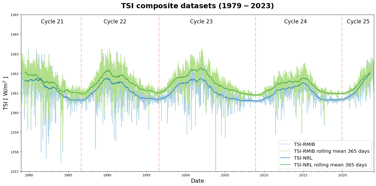
Use case 2: Side-by-side composite products#
The existing 44+ year TSI Climate Data Record (CDR) is the result of several overlapping TSI instruments onboard different satellites. Another well-known composite TSI data are produced by the Naval Research Laboratory (NRL). Each organization collects TSI measurements from various satellite instruments and combines them to create a composite dataset that represents the overall TSI variations over time. In this usecase, we will plot these two composite datasets side-by-side.
Download the NRL dataset, subselecting the time range#
The NRL TSI dataset is made available through LaTiS, which is a data-serving system. It offers multiple methods to access the dataset, providing users with different options to retrieve the data according to their needs or preferences. We then download the selected parameters using a command-line utility wget.
nrl2_tsi_P1D.csv: TSI daily dataset name on the LaTiS server;?time,irradiance: These are the variables that are requested from the dataset: time and irradiance;&formatTime(yyyyMMdd): This is a LaTiS function that formats the time variable as a date string in the format yyyyMMdd.&time>=1979-01-01T00:00: This is another LaTiS function that specifies that you only want data points that have a time value greater than or equal to 1979-01-01T00:00
# download the dataset using wget. -O specifies the output path and filename; -q quiet mode, to disable wget's output
!wget -O $DATADIR/nrl.csv -q "https://lasp.colorado.edu/lisird/latis/dap/nrl2_tsi_P1D.csv?time,irradiance&formatTime(yyyyMMdd)&time>=1979-01-01T00:00"
Load dataset, subselect and calculate a temporal mean#
If you run the Use case 1, C3S RMIB dataset is already saved in the memory. If not, please run the Use case 1 first.
The TSI data is stored in an ASCII file.
We read a dataset using pandas pd.read_csv() into DataFrame. We skip the first line, as it is the name of the columns. We also specify the date format for the first column.
filename_nrl = f'{DATADIR}nrl.csv'
# read the file
data_nrl = pd.read_csv(
    filename_nrl, header=1 ,sep=',', index_col=0, names=["Date", "TSI"],
    parse_dates=[0], date_format='%Y%m%d'
)
Plot data#
We use Matplotlib to create a high-quality plot. We follow the same steps, as in the first use case to plot these two datasets side-by-side.
from matplotlib.font_manager import FontProperties

# Save figure and axes objects to modify later
fig2, ax2 = plt.subplots(1, 1, figsize=[16, 8])

# Actual plotting of the NRL data and the RMIB data
data_nrl.TSI.rolling(window=1).mean().plot(ax=ax2, color="#a6cee3")
data.TSI.rolling(window=1).mean().plot(ax=ax2, color="#b2df8a")
# Then 12-month rolling mean
data_nrl.TSI.rolling(window=365, center=True).mean().plot(ax=ax2, color="#1f78b4")
data.TSI.rolling(window=365, center=True).mean().plot(ax=ax2, color="#33a02c")


# Adding title, x,y labels, and legend at lower right corner
ax2.set_ylim(1357,1365)
ax2.set_title('$\\bf{TSI\\ composite\\ datasets\\ (1979-2023)}$',fontsize=22, pad = 20)

ax2.set_ylabel('TSI [ W/m$^2$ ]',fontsize=17,)
ax2.set_xlabel('Date',fontsize=17)
ax2.legend(
    ["TSI-RMIB", "TSI-RMIB rolling mean 365 days", "TSI-NRL", "TSI-NRL rolling mean 365 days"],
    loc="lower right",
    fontsize='x-large'
)

# Adding vertical lines and labels to distinguish solar cycles
ax2.axvline(pd.to_datetime('1986-09-01'), color="#fb9a99", linestyle="-.")
ax2.axvline(pd.to_datetime('1996-08-01'), color="#fb9a99", linestyle="-.")
ax2.axvline(pd.to_datetime('2008-12-01'), color="#fb9a99", linestyle="-.")
ax2.axvline(pd.to_datetime('2019-12-01'), color="#fb9a99", linestyle="-.")
ax2.text(pd.to_datetime('1983-01-01'), 1364.5, "Cycle 21", ha="center", va="bottom", color="k", fontsize=16)
ax2.text(pd.to_datetime('1991-01-01'), 1364.5, "Cycle 22", ha="center", va="bottom", color="k", fontsize=16)
ax2.text(pd.to_datetime('2002-01-01'), 1364.5, "Cycle 23", ha="center", va="bottom", color="k", fontsize=16)
ax2.text(pd.to_datetime('2014-01-01'), 1364.5, "Cycle 24", ha="center", va="bottom", color="k", fontsize=16)
ax2.text(pd.to_datetime('2022-01-01'), 1364.5, "Cycle 25", ha="center", va="bottom", color="k", fontsize=16)

plt.tight_layout()
plt.show()

# and save the figure
fig2.savefig('Example_2_TSI_SideBySide.png', dpi=300, bbox_inches='tight')
Get more information about Earth Radiation Budget:#
Acknowledgments#
The results presented in this document rely on data from the Naval Research Laboratory Total Solar Irradiance 2 (NRLTSI2) model described in Coddington et al. 2016 (https://doi.org/10.1175/BAMS-D-14-00265.1). These data were accessed via the LASP Interactive Solar Irradiance Datacenter (LISIRD) (https://lasp.colorado.edu/lisird/).
References#
Clerbaux N., (2023) Earth Radiation Budget TSI TOA. Copernicus Climate Change Service. https://confluence.ecmwf.int/x/AFMiEg
Dewitte, S., & Nevens, S. (2016). The Total Solar Irradiance Climate Data Record. The Astrophysical Journal, 830(1), 25. https://doi.org/10.3847/0004-637X/830/1/25.
Clerbaux, N., Velazquez Blazquez, A. (RMIB), 2023, C3S Earth Radiation Budget TSI Service: Product User Guide and Specification. Copernicus Climate Change Service, Document ref. C3S2_D312a_Lot1.2.2.6-v1.0_202303_PUGS_ECVEarthRadiationBudget_v1.1 https://confluence.ecmwf.int/x/KFMiEg