Explore data on glacier mass change available on the Climate Data Store

In this notebook we will use the Climate Data Store (CDS) glacier mass change dataset “Glacier mass change gridded data from 1976 to present derived from the Fluctuations of Glaciers Database” to explore global glacier mass changes over the last 5 decades.

We will start by accessing the glacier mass change dataset from the CDS, read and inspect the annual gridded netCDF4 files.

Then, we will plot the gridded annual glacier mass changes on a global map and make an animation for the entire time series.

Finaly we will explore different ways of plotting the annual time series of global mass change as mean annual mass change rates and uncertainties, as annual climate warming stripes and as total cumulative global mass changes for the full time period.

Initialize Python environment

# Import standard libraries
import zipfile
# 
# Import third party libraries

import cartopy.crs
import cdsapi

import IPython
import matplotlib.animation
import matplotlib.colors
import matplotlib.patches
import matplotlib.pyplot
import pandas
import xarray

# Ignore distracting warnings
import warnings
warnings.filterwarnings('ignore')

Data description

This notebook uses the glacier mass change Climate Data Record (CDR) “Glacier mass change gridded data from 1976 to present derived from the Fluctuations of Glaciers Database” available through the C3S Glacier Change Service Climate Data Store (CDS).

The Glacier Change Service addresses the Glacier Essential Climate Variable (ECV). The glacier mass change CDR consists of a global gridded product of annual glacier mass changes in gigatonnes (Gt) at a 0.5° x 0.5° (latitude, longitude) spatial resolution based on glacier change observations covering the hydrological years from 1975/76 to 2021/23. The Glacier mass change dataset was computed by combining the temporal variability from glaciological in-situ glacier observations with the multiannual to decadal trends from airborne and spaceborne geodetic glacier mass change observations. It builds upon individual glaciers glaciological and geodetic time series available from the latest version of the Fluctuations of Glaciers (FoG) database produced by the World Glacier Monitoring Service (WGMS) and individual glacier areas from the Randolph Glacier Inventory (RGI version 6.0).

The theoretical basis of the Glacier CDR is described in the CDS dataset documentation (Algorithm Theoretical Basis Document (ATBD), Target Requirements and Gap Analysis Document (TRGAD) and Product Quality Assessment Report (PQAR)). The glaciological and geodetic time series used as input data are extensively discussed in WGMS (2024) and in Zemp et al. (2013, 2015, 2019).

Download data

We will use the Climate Data Store (CDS) API to download the glacier mass change dataset.

NOTE: To use the CDS API, you first need to register using your ECMWF account (if not already), find your UID and API key on your acount page, and fill them in below.

# Download data from the CDS
c = cdsapi.Client()
c.retrieve(
    name='derived-gridded-glacier-mass-change',
    request={
        'variable': 'glacier_mass_change',
        'product_version': 'wgms_fog_2022_09',
        'format': 'zip',
        'hydrological_year': [
            '1975_76', '1976_77', '1977_78',
            '1978_79', '1979_80', '1980_81',
            '1981_82', '1982_83', '1983_84',
            '1984_85', '1985_86', '1986_87',
            '1987_88', '1988_89', '1989_90',
            '1990_91', '1991_92', '1992_93',
            '1993_94', '1994_95', '1995_96',
            '1996_97', '1997_98', '1998_99',
            '1999_20', '2000_01', '2001_02',
            '2002_03', '2003_04', '2004_05',
            '2005_06', '2006_07', '2007_08',
            '2008_09', '2009_10', '2010_11',
            '2011_12', '2012_13', '2013_14',
            '2014_15', '2015_16', '2016_17',
            '2017_18', '2018_19', '2019_20',
            '2020_21',
        ],
    },
    target='glacier_mass_change.zip'
)

2024-09-30 14:33:05,885 INFO [2024-04-29T00:00:00] Version WGMS-FOG-2022-09 will be deprecated in the near future. Users are advised to use the latest version.
2024-09-30 14:33:05,886 INFO Request ID is 01079521-60d3-4ba0-96da-1be58d7c6239
2024-09-30 14:33:05,955 INFO status has been updated to accepted
2024-09-30 14:33:09,821 INFO status has been updated to successful

'glacier_mass_change.zip'

Since the data is downloaded as a zip file, we have to first unzip it.

with zipfile.ZipFile('glacier_mass_change.zip', 'r') as file:
    file.extractall('glacier_mass_change')

Read and inspect data

The data are formatted as multiple netCDF4 files, one for each year, but they can be read as a single dataset using xarray.

ds = xarray.open_mfdataset('glacier_mass_change/*.nc4')
ds

<xarray.Dataset>
Dimensions:      (time: 45, lat: 360, lon: 720)
Coordinates:
  * time         (time) datetime64[ns] 1976-01-01 1977-01-01 ... 2021-01-01
  * lat          (lat) float64 89.75 89.25 88.75 88.25 ... -88.75 -89.25 -89.75
  * lon          (lon) float64 -179.8 -179.2 -178.8 -178.2 ... 178.8 179.2 179.8
Data variables:
    Glacier      (time, lat, lon) float64 dask.array<chunksize=(1, 360, 720), meta=np.ndarray>
    Uncertainty  (time, lat, lon) float64 dask.array<chunksize=(1, 360, 720), meta=np.ndarray>
Attributes:
    title:         Global gridded annual glacier mass change product
    project:       Copernicus Climate Change Service (C3S) Essential Climate ...
    data_version:  version-wgms-fog-2022-09
    institution:   World Glacier Monitoring Service - Geography Department - ...
    created_by:    Dr. Ines Dussaillant   ines.dussaillant@geo.uzh.ch
    references:    Fluctuation of Glagiers (FoG) database version wgms-fog-20...
    citation:      
    Conventions:   CF Version CF-1.8
    comment:       Brief data description:Horizontal resolution:\t0.5° (latit...

xarray.Dataset

• Dimensions:
  • time: 45
  • lat: 360
  • lon: 720
• Coordinates: (3)
  • time
    (time)
    datetime64[ns]
    1976-01-01 ... 2021-01-01

    standard_name :

    time

    long_name :

    time axis

    array(['1976-01-01T00:00:00.000000000', '1977-01-01T00:00:00.000000000',
           '1978-01-01T00:00:00.000000000', '1979-01-01T00:00:00.000000000',
           '1980-01-01T00:00:00.000000000', '1981-01-01T00:00:00.000000000',
           '1982-01-01T00:00:00.000000000', '1983-01-01T00:00:00.000000000',
           '1984-01-01T00:00:00.000000000', '1985-01-01T00:00:00.000000000',
           '1986-01-01T00:00:00.000000000', '1987-01-01T00:00:00.000000000',
           '1988-01-01T00:00:00.000000000', '1989-01-01T00:00:00.000000000',
           '1990-01-01T00:00:00.000000000', '1991-01-01T00:00:00.000000000',
           '1992-01-01T00:00:00.000000000', '1993-01-01T00:00:00.000000000',
           '1994-01-01T00:00:00.000000000', '1995-01-01T00:00:00.000000000',
           '1996-01-01T00:00:00.000000000', '1997-01-01T00:00:00.000000000',
           '1998-01-01T00:00:00.000000000', '1999-01-01T00:00:00.000000000',
           '2001-01-01T00:00:00.000000000', '2002-01-01T00:00:00.000000000',
           '2003-01-01T00:00:00.000000000', '2004-01-01T00:00:00.000000000',
           '2005-01-01T00:00:00.000000000', '2006-01-01T00:00:00.000000000',
           '2007-01-01T00:00:00.000000000', '2008-01-01T00:00:00.000000000',
           '2009-01-01T00:00:00.000000000', '2010-01-01T00:00:00.000000000',
           '2011-01-01T00:00:00.000000000', '2012-01-01T00:00:00.000000000',
           '2013-01-01T00:00:00.000000000', '2014-01-01T00:00:00.000000000',
           '2015-01-01T00:00:00.000000000', '2016-01-01T00:00:00.000000000',
           '2017-01-01T00:00:00.000000000', '2018-01-01T00:00:00.000000000',
           '2019-01-01T00:00:00.000000000', '2020-01-01T00:00:00.000000000',
           '2021-01-01T00:00:00.000000000'], dtype='datetime64[ns]')

  • lat
    (lat)
    float64
    89.75 89.25 88.75 ... -89.25 -89.75

    standard_name :

    latitude

    long_name :

    latitude

    units :

    degrees_north

    valid_min :

    -89.75

    valid_max :

    89.75

    array([ 89.75,  89.25,  88.75, ..., -88.75, -89.25, -89.75])

  • lon
    (lon)
    float64
    -179.8 -179.2 ... 179.2 179.8

    standard_name :

    longitude

    long_name :

    longitude

    units :

    degrees_east

    valid_min :

    -179.75

    valid_max :

    179.75

    array([-179.75, -179.25, -178.75, ...,  178.75,  179.25,  179.75])

• Data variables: (2)
  • Glacier
    (time, lat, lon)
    float64
    dask.array<chunksize=(1, 360, 720), meta=np.ndarray>

    standard_name :

    glacier_mass_change

    long_name :

    glacier_mass_change

    units :

    Gt

    Array Chunk Bytes 88.99 MiB 1.98 MiB Shape (45, 360, 720) (1, 360, 720) Dask graph 45 chunks in 91 graph layers Data type float64 numpy.ndarray

  • Uncertainty
    (time, lat, lon)
    float64
    dask.array<chunksize=(1, 360, 720), meta=np.ndarray>

    standard_name :

    uncertainty

    long_name :

    glacier_mass_change_uncertainty

    units :

    Gt

    Array Chunk Bytes 88.99 MiB 1.98 MiB Shape (45, 360, 720) (1, 360, 720) Dask graph 45 chunks in 91 graph layers Data type float64 numpy.ndarray

• Indexes: (3)
  • time
    PandasIndex

    PandasIndex(DatetimeIndex(['1976-01-01', '1977-01-01', '1978-01-01', '1979-01-01',
                   '1980-01-01', '1981-01-01', '1982-01-01', '1983-01-01',
                   '1984-01-01', '1985-01-01', '1986-01-01', '1987-01-01',
                   '1988-01-01', '1989-01-01', '1990-01-01', '1991-01-01',
                   '1992-01-01', '1993-01-01', '1994-01-01', '1995-01-01',
                   '1996-01-01', '1997-01-01', '1998-01-01', '1999-01-01',
                   '2001-01-01', '2002-01-01', '2003-01-01', '2004-01-01',
                   '2005-01-01', '2006-01-01', '2007-01-01', '2008-01-01',
                   '2009-01-01', '2010-01-01', '2011-01-01', '2012-01-01',
                   '2013-01-01', '2014-01-01', '2015-01-01', '2016-01-01',
                   '2017-01-01', '2018-01-01', '2019-01-01', '2020-01-01',
                   '2021-01-01'],
                  dtype='datetime64[ns]', name='time', freq=None))

  • lat
    PandasIndex

    PandasIndex(Index([ 89.75,  89.25,  88.75,  88.25,  87.75,  87.25,  86.75,  86.25,  85.75,
            85.25,
           ...
           -85.25, -85.75, -86.25, -86.75, -87.25, -87.75, -88.25, -88.75, -89.25,
           -89.75],
          dtype='float64', name='lat', length=360))

  • lon
    PandasIndex

    PandasIndex(Index([-179.75, -179.25, -178.75, -178.25, -177.75, -177.25, -176.75, -176.25,
           -175.75, -175.25,
           ...
            175.25,  175.75,  176.25,  176.75,  177.25,  177.75,  178.25,  178.75,
            179.25,  179.75],
          dtype='float64', name='lon', length=720))

• Attributes: (9)

  title :

  Global gridded annual glacier mass change product

  project :

  Copernicus Climate Change Service (C3S) Essential Climate Variable products derived from observations C3S2_312a Lot No 4: Land Hydrology and Cryosphere

  data_version :

  version-wgms-fog-2022-09

  institution :

  World Glacier Monitoring Service - Geography Department - University of Zurich - Zurich - Switzerland

  created_by :

  Dr. Ines Dussaillant ines.dussaillant@geo.uzh.ch

  references :

  Fluctuation of Glagiers (FoG) database version wgms-fog-2022-09

  citation :

  Conventions :

  CF Version CF-1.8

  comment :

  Brief data description:Horizontal resolution: 0.5° (latitude - longitude), GCS_WGS_1984 Temporal resolution: Annual, hydrological year Temporal coverage: 1975/76-2020/21Observational sample: 96% of world glaciers with valid observations

Each time value contains a date, but represents a hydrological year. For example, 1976-01-01 represents the 1975–1976 hydrological year. To simplify what follows, we reduce each time to the end year of the hydrological year.

ds['time'] = [date.year for date in ds['time'].values.astype('datetime64[D]').tolist()]
ds['time']

<xarray.DataArray 'time' (time: 45)>
array([1976, 1977, 1978, 1979, 1980, 1981, 1982, 1983, 1984, 1985, 1986, 1987,
       1988, 1989, 1990, 1991, 1992, 1993, 1994, 1995, 1996, 1997, 1998, 1999,
       2001, 2002, 2003, 2004, 2005, 2006, 2007, 2008, 2009, 2010, 2011, 2012,
       2013, 2014, 2015, 2016, 2017, 2018, 2019, 2020, 2021])
Coordinates:
  * time     (time) int64 1976 1977 1978 1979 1980 ... 2017 2018 2019 2020 2021

xarray.DataArray

'time'

• time: 45

• 1976 1977 1978 1979 1980 1981 1982 ... 2016 2017 2018 2019 2020 2021

  array([1976, 1977, 1978, 1979, 1980, 1981, 1982, 1983, 1984, 1985, 1986, 1987,
         1988, 1989, 1990, 1991, 1992, 1993, 1994, 1995, 1996, 1997, 1998, 1999,
         2001, 2002, 2003, 2004, 2005, 2006, 2007, 2008, 2009, 2010, 2011, 2012,
         2013, 2014, 2015, 2016, 2017, 2018, 2019, 2020, 2021])

• Coordinates: (1)
  • time
    (time)
    int64
    1976 1977 1978 ... 2019 2020 2021

    array([1976, 1977, 1978, 1979, 1980, 1981, 1982, 1983, 1984, 1985, 1986, 1987,
           1988, 1989, 1990, 1991, 1992, 1993, 1994, 1995, 1996, 1997, 1998, 1999,
           2001, 2002, 2003, 2004, 2005, 2006, 2007, 2008, 2009, 2010, 2011, 2012,
           2013, 2014, 2015, 2016, 2017, 2018, 2019, 2020, 2021])

• Indexes: (1)
  • time
    PandasIndex

    PandasIndex(Index([1976, 1977, 1978, 1979, 1980, 1981, 1982, 1983, 1984, 1985, 1986, 1987,
           1988, 1989, 1990, 1991, 1992, 1993, 1994, 1995, 1996, 1997, 1998, 1999,
           2001, 2002, 2003, 2004, 2005, 2006, 2007, 2008, 2009, 2010, 2011, 2012,
           2013, 2014, 2015, 2016, 2017, 2018, 2019, 2020, 2021],
          dtype='int64', name='time'))

• Attributes: (0)

Plot mass change on a map

Static map for one year

We use matplotlib and cartopy to make a map of glacier mass change for one year.

# Select year
YEAR = 2021

# Create a map with a plate carrée projection
figure = matplotlib.pyplot.figure(figsize=(12, 6))
axis = matplotlib.pyplot.axes(projection=cartopy.crs.PlateCarree())

# Add title
axis.set_title(f"Hydrological year {YEAR - 1}–{YEAR}")

# Add latitude, longitude gridlines
axis.gridlines(draw_labels=True, alpha=0.25, linestyle=':', color='white')

# Add white continents against a gray background
axis.set_facecolor('darkgray')
axis.add_feature(cartopy.feature.LAND, facecolor='lightgray')

# Define range and ticks of color scale
ticks = [-1, -0.1, -0.01, 0, 0.01, 0.1, 1]

# Plot mass loss in red and gain in blue
# A log scale is used for colors to highlight differences between regions
im = matplotlib.pyplot.pcolormesh(
    ds['lon'],
    ds['lat'],
    ds['Glacier'].loc[YEAR],
    cmap='RdBu',
    norm=matplotlib.colors.SymLogNorm(
        vmin=ticks[0], vmax=ticks[-1], linthresh=0.01
    )
)

# Add a colorbar with custom ticks
cbar = matplotlib.pyplot.colorbar(
    im,
    fraction=0.025,
    pad=0.05,
    label='Glacier mass change (Gt)',
    ticks=ticks
)
cbar.ax.set_yticklabels([f'< {ticks[0]}', *ticks[1:-1], f'> {ticks[-1]}'])

# Show plot
figure.tight_layout(pad=0)
matplotlib.pyplot.show()

# Print a text describing the figure
txt=(f"Figure 1: Global gridded annual glacier mass-changes (in Gt per year). Visualization example of the gridded glacier change product" 
"\n"
f"for the hydrological year {YEAR - 1}–{YEAR}, spatially distributed in a global regular grid of 0.5° (latitude/longitude).")
print(txt)

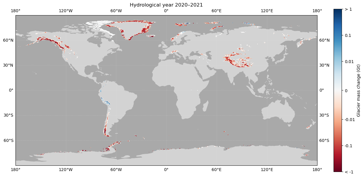
Figure 1: Global gridded annual glacier mass-changes (in Gt per year). Visualization example of the gridded glacier change product
for the hydrological year 2020–2021, spatially distributed in a global regular grid of 0.5° (latitude/longitude).

Animation for all years

Using the map above as a template, we create a map for each year and display them in an animation. Make sure to run this cell immediately after the cell above.

The resulting animation shows the global gridded annual glacier mass-changes (in Gt per year) for the hydrological years from 1975/76 to 2021/22.

# Define the animation parameters
def animate(time_index: int) -> None:
    im.set_array(ds['Glacier'][time_index].values.ravel())
    year = ds['time'].values[time_index]
    axis.set_title(f"Hydrological year {year - 1}–{year}")

# Plot static maps for every year and create the animation
animation = matplotlib.animation.FuncAnimation(
    figure,
    func=animate,
    frames=ds['time'].size,
    interval=500  # ms
)

# Display animation
IPython.display.HTML(animation.to_jshtml())

Once Loop Reflect

Plot timeseries of global mass change

Compute mean of global change

The global mass change is the sum of the mass changes reported for each spatial grid cell. We compute it by summing mass change across the latitude (lat) and longitude (lon) dimensions.

# compute mean global glacier mass-change
global_change_mean = ds.sum(dim=['lat', 'lon'])['Glacier']

Compute standard deviation of global change

If we assume that the mass changes for which we computed the sum above are uncorrelated, the standard deviation of their sum is the square root of the sum of the squares of their standard deviatons:

\( f = \textstyle\sum_i m_i \\ \sigma_f = \sqrt {\textstyle\sum_i \sigma_i^2} \)

See Wikipedia: Propagation of uncertainty for more information.

We divide the uncertainty by 1.96 below because the authors report that this value is 1.96 \(\sigma\) (equivalent to a 95% confidence interval for a normal distribution).

# compute standard deviation of global glacier mass-change
global_change_std = ((ds['Uncertainty'] / 1.96) ** 2).sum(dim=['lat', 'lon']) ** 0.5

View timeseries as a table

We use pandas to tabulate the mean and standard deviation computed above.

# view global annual mass-change time series and standard deviation as a table
print( "Table 1: Yearly mean global glacier mass-changes (in Gt per year) and their related standard deviation (std)" )
pandas.DataFrame({
    'year': ds['time'],
    'mean': global_change_mean,
    'std': global_change_std
})

Table 1: Yearly mean global glacier mass-changes (in Gt per year) and their related standard deviation (std)

	year	mean	std
0	1976	90.711681	29.427761
1	1977	-9.916545	29.827922
2	1978	-7.919292	29.135105
3	1979	-20.050397	29.187522
4	1980	80.726975	29.364131
5	1981	86.211509	31.511226
6	1982	-26.793842	28.662013
7	1983	140.430476	28.653894
8	1984	-29.203053	28.564248
9	1985	32.698277	28.637171
10	1986	69.848798	27.594141
11	1987	134.985990	27.841201
12	1988	12.617256	27.050033
13	1989	-18.082409	26.847752
14	1990	-248.443006	27.656334
15	1991	-143.120973	26.829816
16	1992	133.672195	26.663257
17	1993	-87.847944	26.652052
18	1994	-89.210215	26.410071
19	1995	-200.446107	26.171569
20	1996	-83.870737	25.528025
21	1997	-327.845908	24.748657
22	1998	-158.643409	24.510523
23	1999	-229.454042	24.563616
24	2001	-162.298628	12.494367
25	2002	-160.765585	9.332476
26	2003	-190.294174	14.942672
27	2004	-379.090233	11.315378
28	2005	-403.113326	11.086587
29	2006	-285.326933	11.548195
30	2007	-340.458477	11.253159
31	2008	-174.674641	11.426205
32	2009	-257.799645	8.735710
33	2010	-297.322767	11.295674
34	2011	-390.143004	9.291715
35	2012	-231.262888	9.896819
36	2013	-254.336647	11.493179
37	2014	-165.881781	8.630415
38	2015	-219.722406	8.452308
39	2016	-378.749650	9.953543
40	2017	-273.700155	7.438282
41	2018	-217.651581	12.309113
42	2019	-500.817056	8.147666
43	2020	-398.682773	7.292266
44	2021	-336.283551	8.161970

Plot timeseries

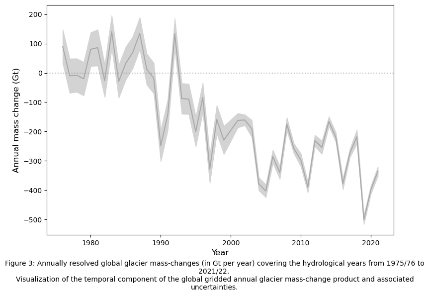
We use matplotlib to plot the mean and uncertainty of the global mass change for each year.

# Configure the figure
figure, axis = matplotlib.pyplot.subplots(1, 1, figsize=(9, 6))
axis.set_ylabel('Annual mass change (Gt)', fontsize=12)
axis.set_xlabel('Year', fontsize=12)

# Plot a horizontal line at 0 change
axis.axhline(y=0, alpha=0.5, linestyle=':', color='gray')

# Plot the uncertainty as 1.96 standard deviations below and above the mean
axis.fill_between(
    x=ds['time'],
    y1=global_change_mean - global_change_std * 1.96,
    y2=global_change_mean + global_change_std * 1.96,
    color='lightgray'
)

# Plot the mean as a line
axis.plot(
    ds['time'],
    global_change_mean,
    color='darkgray'
)

txt=("Figure 3: Annually resolved global glacier mass-changes (in Gt per year) covering the hydrological years from 1975/76 to 2021/22. " 
"\n"
"Visualization of the temporal component of the global gridded annual glacier mass-change product and associated uncertainties.")

matplotlib.pyplot.figtext(0.5, -0.07, txt, wrap=True, horizontalalignment='center', fontsize=10)

# Show figure
matplotlib.pyplot.show()

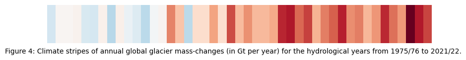
We can also plot this in the style of the popular climate warming stripes.

# Configure the figure
figure, axis = matplotlib.pyplot.subplots(1, 1, figsize=(10, 1))
axis.set_xlim(0, global_change_mean.size)
axis.set_axis_off()

# Define a red (negative) to blue (positive) colorscale
colormap = matplotlib.pyplot.get_cmap('RdBu')

# Saturate colors at -500 and +500 Gt
normalizer = matplotlib.colors.Normalize(vmin=-500, vmax=500)

# Create a colored rectangle for each year
for i, value in enumerate(global_change_mean):
    axis.add_patch(matplotlib.patches.Rectangle(
        xy=(i, 0), width=1, height=1, facecolor=colormap(normalizer(value))
    ))

txt=("Figure 4: Climate stripes of annual global glacier mass-changes (in Gt per year) for the hydrological years from 1975/76 to 2021/22." )

matplotlib.pyplot.figtext(0.5, -0.1, txt, wrap=True, horizontalalignment='center', fontsize=10)

# Show figure
matplotlib.pyplot.show()

Plot total global mass change

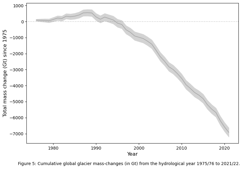
Rather than plot the annual mass change, we would like to plot the total mass change accumulated from the beginning of the series to each subsequent year. To do so, we take the cumulative sum of the annual mass changes calculated above. To calculate the standard deviation of this total, we apply the same principle as before.

# compute cumulative global glacier mass-changes and total standard deviation
global_change_total = global_change_mean.cumsum()
global_change_total_std = (global_change_std ** 2).cumsum() ** 0.5

Again, we can use pandas to tabulate the total and its standard deviation.

# view the cummulative global glacier mass-change time series and their standard deviation as a table
print( "Table 2: Cumulative global glacier mass-changes (in Gt per year) and their related standard deviation (total_std)" )
pandas.DataFrame({
    'year': ds['time'],
    'total': global_change_total,
    'total_std': global_change_total_std
})

Table 2: Cumulative global glacier mass-changes (in Gt per year) and their related standard deviation (total_std)

	year	total	total_std
0	1976	90.711681	29.427761
1	1977	80.795136	41.901051
2	1978	72.875844	51.034816
3	1979	52.825448	58.791699
4	1980	133.552423	65.716939
5	1981	219.763931	72.881228
6	1982	192.970089	78.314650
7	1983	333.400565	83.392026
8	1984	304.197512	88.148433
9	1985	336.895789	92.683514
10	1986	406.744587	96.704035
11	1987	541.730577	100.632017
12	1988	554.347833	104.204161
13	1989	536.265424	107.607198
14	1990	287.822419	111.104373
15	1991	144.701446	114.297947
16	1992	278.373640	117.366733
17	1993	190.525696	120.354817
18	1994	101.315481	123.218399
19	1995	-99.130625	125.967158
20	1996	-183.001362	128.527837
21	1997	-510.847270	130.888888
22	1998	-669.490679	133.164059
23	1999	-898.944721	135.410627
24	2001	-1061.243349	135.985834
25	2002	-1222.008934	136.305694
26	2003	-1412.303108	137.122302
27	2004	-1791.393341	137.588384
28	2005	-2194.506667	138.034329
29	2006	-2479.833600	138.516557
30	2007	-2820.292077	138.972912
31	2008	-2994.966718	139.441846
32	2009	-3252.766363	139.715214
33	2010	-3550.089130	140.171086
34	2011	-3940.232134	140.478715
35	2012	-4171.495022	140.826902
36	2013	-4425.831670	141.295115
37	2014	-4591.713451	141.558446
38	2015	-4811.435857	141.810560
39	2016	-5190.185507	142.159446
40	2017	-5463.885663	142.353911
41	2018	-5681.537244	142.885095
42	2019	-6182.354299	143.117207
43	2020	-6581.037072	143.302868
44	2021	-6917.320623	143.535117

Finally, we use matplotlib to plot the total and its uncertainty.

# Configure the figure
figure, axis = matplotlib.pyplot.subplots(1, 1, figsize=(9, 6))
start_year = ds['time'].values[0] - 1
axis.set_ylabel(f"Total mass change (Gt) since {start_year}", fontsize=12)
axis.set_xlabel('Year', fontsize=12)

# Plot a horizontal line at 0 change
axis.axhline(y=0, alpha=0.5, linestyle=':', color='gray')

# Plot the uncertainty as 1.96 standard deviations
axis.fill_between(
    x=ds['time'],
    y1=global_change_total - global_change_total_std * 1.96,
    y2=global_change_total + global_change_total_std * 1.96,
    color='lightgray'
)

# Plot the mean as a line
axis.plot(
    ds['time'],
    global_change_total,
    color='darkgray'
)

txt=("Figure 5: Cumulative global glacier mass-changes (in Gt) from the hydrological year 1975/76 to 2021/22.")

matplotlib.pyplot.figtext(0.5, -0.01, txt, wrap=True, horizontalalignment='center', fontsize=10)

# Show figure
matplotlib.pyplot.show()

What have you learned?

You ready to use the Climate Data Store (CDS) glacier mass change dataset to explore how global glaciers have evolved over the last 5 decades.

You know how to plot global glacier-changes in a map and observe how the worlds glaciers have evolved year by year on an animated map from 1976 to 2021.

You also know how to plot global glacier mass-changes in different ways, as mean annual mass change-rates, climate warming stripes or as the total cumulative global mass changes since 1976.

Enjoy playing with the glacier mass change dataset!