Analysis of Projected versus Historical Climatology with CORDEX Data

Analysis of Projected versus Historical Climatology with CORDEX Data#

About#

This notebook is a practical introduction to CORDEX regional climate model data on single levels. CORDEX data are available for 14 regional domains and variable spatial resolutions, from 0.11 x 0.11 degrees up to 0.44 x 0.44 degrees. This workflow will demonstrate how to compute the difference in the air temperature climatology for 2071-2100 (according to a projected scenario) relative to the reference period 1971-2000 in Africa, with a spatial resolution of 0.44 x 0.44 degrees.

We will use the historical experiment to compute the past climatology and repeat the steps to compute the projected climatology according to the scenario RCP4.5. Finally, we will take the difference between the two in order to assess the extent of change. This is called the “delta method” which takes the climate change signal as the difference between the future and past considering that the model biases are the same and can therefore be removed with the subtraction.

This particular example uses data from the Canadian Regional Climate Model CCCma_CanRCM4, with lateral boundary conditions from the Global Climate Model (GCM) CanESM2, also Canadian. This coupled model is referred to as CanRCM4 - CanESM2. See here a full list of models included in the CDS-CORDEX subset.

Note: The workflow uses a specific model, scenario and geographical area, but you can use any model, scenario or domain, and indeed any period or variable. To have a more accurate idea of projected climate change, it is typical to calculate an ensemble of multiple models. Only for the sake of simplicity do we focus on one model.

In general, CORDEX experiments can be divided into three main categories:

Evaluation: model simulations for the past with imposed “perfect” lateral boundary conditions following ERA-Interim reanalysis (1979-2015).
Historical: Historical experiments cover the period where modern climate observations exist. These experiements show how the RCMs perform for the past climate when forced by the Global Circulation Model (GCM) and can be used as a reference period for comparison with scenario runs for the future.
Scenario experiments RCP2.6, RCP4.5, RCP8.5: ensemble of CORDEX climate projection experiments driven by boundary conditions from GCMs using RCP (Representative Concentration Pathways) forcing scenarios. The scenarios used here are RCP 2.6, 4.5 and 8.5, which provide different pathways of the future climate forcing.

Learn here more about CORDEX experiments in the Copernicus Climate Data Store (CDS).

The notebook has the following outline:

Request data from the CDS programmatically with the CDS API
Unzip the downloaded data files
Compute CORDEX historical climatology for reference period 1971-2000
Compute CORDEX projected climatology for target period 2071-2100 based on scenario RCP4.5
Compute and visualize the climate change signal

Data#

This notebook introduces you to CORDEX regional climate model data on single levels. The data used in the notebook has the following specifications:

Data: CORDEX regional climate model data on single levels - Experiment: Historical
Temporal coverage: 1 Jan 1971 to 31 Dec 2000
Spatial coverage: Domain: Africa
Format: NetCDF in zip archives

Data: CORDEX regional climate model data on single levels - Experiment: RCP4.5
Temporal coverage: 1 Jan 2071 to 31 Dec 2100
Spatial coverage: Domain: Africa
Format: NetCDF in zip archives

Run the tutorial via free cloud platforms:

Install CDS API via pip#

!pip install cdsapi

Load libraries#

# CDS API
import cdsapi

# Libraries for working with multidimensional arrays
import numpy as np
import xarray as xr

# Libraries for plotting and visualising data
import matplotlib.path as mpath
import matplotlib.pyplot as plt
from matplotlib.colors import ListedColormap, LinearSegmentedColormap
import cartopy.crs as ccrs
from cartopy.mpl.gridliner import LONGITUDE_FORMATTER, LATITUDE_FORMATTER
import cartopy.feature as cfeature

# Other libraries (e.g. paths, filenames, zipfile extraction)
from glob import glob
from pathlib import Path
from os.path import basename
import zipfile
import urllib3 
urllib3.disable_warnings() # Disable "InsecureRequestWarning" 
                           # for data download via API

Request data from the CDS programmatically with the CDS API#

The first step is to request data from the Climate Data Store programmatically with the help of the CDS API. Let us make use of the option to manually set the CDS API credentials. First, you have to define two variables: URL and KEY which build together your CDS API key. Below, you have to replace the ######### with your personal CDS key. Please find here your personal CDS key.

URL = 'https://cds.climate.copernicus.eu/api/v2'
KEY = '##################################'

DATADIR = './'

The next step is then to request the data with the help of the CDS API. Below are two blocks of code for the following data requests:

Historical experiment: Daily aggregated historical 2m air temperature (from the CanRCM4 - CanESM2 model) from 1971 to 2000 for Africa.
RCP4.5 experiment: Daily aggregated RCP4.5 projections of 2m air temperature (from the CanRCM4 - CanESM2 model) from 2071 to 2100 for Africa

Note: Before you run the cells below, the terms and conditions on the use of the data need to have been accepted in the CDS. You can view and accept these conditions by logging into the CDS, searching for the dataset, then scrolling to the end of the Download data section.

c = cdsapi.Client(url=URL, key=KEY)

c.retrieve(
    'projections-cordex-domains-single-levels',
    {
        'format': 'zip',
        'domain': 'africa',
        'experiment': 'historical',
        'horizontal_resolution': '0_44_degree_x_0_44_degree',
        'temporal_resolution': 'daily_mean',
        'variable': '2m_air_temperature',
        'gcm_model': 'cccma_canesm2',
        'rcm_model': 'cccma_canrcm4',
        'ensemble_member': 'r1i1p1',
        'start_year': ['1971', '1976', '1981', '1986', '1991', '1996'],
        'end_year': ['1975', '1980', '1985', '1990', '1995', '2000'],
    },
    f'{DATADIR}1971-2000_cordex_historical_africa.zip')

2022-03-03 22:13:47,034 INFO Welcome to the CDS
2022-03-03 22:13:47,049 INFO Sending request to https://cds.climate.copernicus.eu/api/v2/resources/projections-cordex-domains-single-levels
2022-03-03 22:13:47,142 INFO Request is queued
2022-03-03 22:13:48,199 INFO Request is running
2022-03-03 22:18:05,397 INFO Request is completed
2022-03-03 22:18:05,400 INFO Downloading https://download-0012.copernicus-climate.eu/cache-compute-0012/cache/data6/dataset-projections-cordex-domains-single-levels-19a7525a-dc2e-4e68-bba7-609414960047.zip to ./cordex/1971-2000_cordex_historical_africa.zip (908.2M)
2022-03-03 22:32:25,835 INFO Download rate 1.1M/s                                                                      

Result(content_length=952308195,content_type=application/zip,location=https://download-0012.copernicus-climate.eu/cache-compute-0012/cache/data6/dataset-projections-cordex-domains-single-levels-19a7525a-dc2e-4e68-bba7-609414960047.zip)

c.retrieve(
    'projections-cordex-domains-single-levels',
    {
        'format': 'zip',
        'domain': 'africa',
        'experiment': 'rcp_4_5',
        'horizontal_resolution': '0_44_degree_x_0_44_degree',
        'temporal_resolution': 'daily_mean',
        'variable': '2m_air_temperature',
        'gcm_model': 'cccma_canesm2',
        'rcm_model': 'cccma_canrcm4',
        'ensemble_member': 'r1i1p1',
        'start_year': ['2071', '2076', '2081', '2086', '2091', '2096'],
        'end_year': ['2075', '2080', '2085', '2090', '2095', '2100'],
    },
    f'{DATADIR}2071-2100_cordex_rcp_4_5_africa.zip')

2022-03-03 22:03:00,724 INFO Welcome to the CDS
2022-03-03 22:03:00,730 INFO Sending request to https://cds.climate.copernicus.eu/api/v2/resources/projections-cordex-domains-single-levels
2022-03-03 22:03:00,863 INFO Request is queued
2022-03-03 22:03:01,925 INFO Request is running
2022-03-03 22:09:19,471 INFO Request is completed
2022-03-03 22:09:19,478 INFO Downloading https://download-0000.copernicus-climate.eu/cache-compute-0000/cache/data3/dataset-projections-cordex-domains-single-levels-b19f6b3d-9012-41cd-98fa-c4820a3daeae.zip to ./cordex/2071-2100_cordex_rcp_4_5_africa.zip (908.1M)
2022-03-03 22:12:09,215 INFO Download rate 5.4M/s                                                                      

Result(content_length=952229444,content_type=application/zip,location=https://download-0000.copernicus-climate.eu/cache-compute-0000/cache/data3/dataset-projections-cordex-domains-single-levels-b19f6b3d-9012-41cd-98fa-c4820a3daeae.zip)

Unzip the downloaded data files#

From the Copernicus Climate Data Store, CORDEX data are available in NetCDF format in compressed archives, either zip or tar.gz. For this reason, before we can load any data, we have to unzip or untar the files. Having downloaded the two experiments historical and RCP4.5 as seperate zip files, we can use the functions from the zipfile Python package to extract the content of a zip file. First, we construct a ZipFile() object and second, we apply the function extractall() to extract the content of the zip file.

Below, the same process is repeated for the two zip files downloaded. We see that the actual data files are disseminated in NetCDF. CORDEX files are generally organised in five year periods. For this reason, for each zip file, six NetCDF files in five year periods are extracted.

cordex_zip_paths = glob(f'{DATADIR}*.zip')

for j in cordex_zip_paths:
    with zipfile.ZipFile(j, 'r') as zip_ref:
        zip_ref.extractall(f'{DATADIR}')

Compute CORDEX future climatology for target period 2071-2100 based on scenario RCP4.5#

Let us now repeat the steps executed for the historical experiment data with the scenario RCP4.5 data. With the projection data for the target period 2071 to 2100, we can compute the projected climatology according to this particular scenario, which can be compared with the historical climatology from the reference period.

Again, we begin with the function open_mfdataset() to load the multiple NetCDF files. The scenario data is also organised into separate files for each 5-year period. These will be concatenated along the time dimension.

ds_2071_2100_projection = xr.open_mfdataset(f'{DATADIR}*CanESM2_rcp45*.nc')

Again we load the data variable tas from the Dataset above into an xarray.DataArray object to facilitate further processing:

tas_2071_2100_projection = ds_2071_2100_projection['tas']

# uncomment the line below before running this cell to view the data characteristics
# tas_2071_2100_projection

Now we will compute the monthly climatology for the target period 2071 to 2100, in the same way as we did for the historical period:

tas_2071_2100_climatology = tas_2071_2100_projection.groupby('time.month').mean()

And finally we convert from degrees Kelvin to Celsius:

tas_2071_2100_climatology_degC = tas_2071_2100_climatology - 273.15

Compute and visualize the climate change signal between the target (2071-2100) and reference (1971-2000) period#

Now, we can compute the difference between the two climatologies. Since both DataArrays have the same structure, we can simply subtract the historical climatology from the projected climatology. The resulting data array has the projected averaged temperature difference for each month.

tas_difference_climatology = tas_2071_2100_climatology - tas_1971_2000_climatology

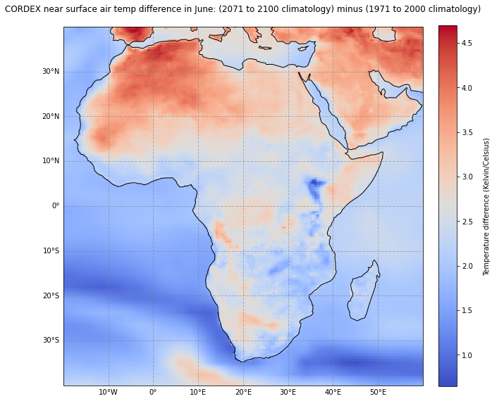
Now, let us visualize the climate change signal between the target (2071-2100) and reference (1971-2000) period for Africa for June. The plotting function below has five main parts:

Initiate the plot: initiate a matplotlib plot with plt.figure and plt.subplot()
Plot the 2D map with pcolormesh: plot the xarray data array as 2D map with the function pcolormesh
Add coast- and gridlines: add additional items to the plot, such as coast- and gridlines
Add title and legend: Set title and legend of the map
Save the figure as png file

We can change the value for the variable month and we see that the near-surface air temperature difference is for some regions more pronounced for some months, e.g. June, compared to others.

month=5

# Initiate the plot
fig = plt.figure(figsize=(10,10))
ax = plt.subplot(1,1,1, projection=ccrs.PlateCarree())

# Plot the 2D map with pcolormesh
im = plt.pcolormesh(tas_difference_climatology.rlon, tas_difference_climatology.rlat,
                   tas_difference_climatology[month,:,:], cmap='coolwarm', transform=ccrs.PlateCarree())

# Add coast- and gridlines
ax.coastlines(color='black')
ax.set_extent([-20,60,-40,40], crs=ccrs.PlateCarree())
gl = ax.gridlines(draw_labels=True, linewidth=1, color='gray', alpha=0.5, linestyle='--')
gl.top_labels = False
gl.right_labels = False

# Add title and legend
ax.set_title('CORDEX near surface air temp difference in June: (2071 to 2100 climatology) minus (1971 to 2000 climatology)\n', fontsize=12)
cbar = plt.colorbar(im,fraction=0.046, pad=0.04)
cbar.set_label('\nTemperature difference (Kelvin/Celsius)\n')

# Save the figure
fig.savefig(f'{DATADIR}TAS_1971-2000_2071-2100_june.png', dpi=300)

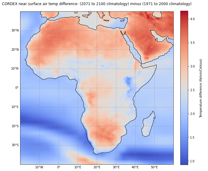
_images/177fb9ead26ebc499ea8095e20702cdcefb0ed3d232318802d34982c7f4094a5.png

As a last step, we repeat the visualization of climate change signal between the target (2071-2100) and reference (1971-2000) period. But this time, we create the average signal for the whole period, not only one month. For this, we have to compute the average over all months with the function mean().

fig = plt.figure(figsize=(10,10))
ax = plt.subplot(1,1,1, projection=ccrs.PlateCarree())

im = plt.pcolormesh(tas_difference_climatology.rlon, tas_difference_climatology.rlat,
                   tas_difference_climatology.mean('month'), cmap='coolwarm', transform=ccrs.PlateCarree())

ax.coastlines(color='black')
ax.set_extent([-20,60,-40,40], crs=ccrs.PlateCarree())
gl = ax.gridlines(draw_labels=True, linewidth=1, color='gray', alpha=0.5, linestyle='--')
gl.top_labels = False
gl.right_labels = False
ax.set_title('CORDEX near surface air temp difference: (2071 to 2100 climatology) minus (1971 to 2000 climatology)\n', fontsize=12)

cbar = plt.colorbar(im,fraction=0.046, pad=0.04)
cbar.set_label('\nTemperature difference (Kelvin/Celsius)\n')

fig.savefig(f'{DATADIR}TAS_1971-2000_2071-2100.png', dpi=300)

_images/b6ea186079c49c772d8ebd5bc3f6d39fb4792f7dda82ce39333491ebf0d5ad5b.png

This project is licensed under APACHE License 2.0. | View on GitHub