Seasonal Forecast Anomalies

Seasonal Forecast Anomalies#

About#

This notebook provides a practical introduction to calculating seasonal forecast anomalies with data from the Copernicus Climate Change Service (C3S). C3S seasonal forecast products are based on data from several state-of-the-art seasonal prediction systems. In this tutorial we shall focus on the ECMWF SEAS5 model, which is one of the forecasting systems available through C3S.

The tutorial will demonstrate how to access real-time forecast data of total precipitation, with a forecast start date in May 2021 and 6 monthly lead times (up to October 2021). Hindcast data for the same start date and lead-time months in the reference period 1993 to 2016 will also be downloaded. The tutorial will then show how to extract a subset area over South Asia for both the forecast and hindcast data. The climate mean for the reference period will be computed and this reference mean will be subtracted from the real-time forecast data to derive monthly anomalies. These will be visualised as both spatial maps and time series. Finally, 3-monthly anomalies will be calculated and visualised in an interactive plot, as a demonstration of how to reproduce similar charts available through C3S.

The notebook has the following outline:

1 - Download data from the CDS
2 - Hindcast data processing: calculate the reference climate mean
3 - Real-time forecasts: calculate seasonal forecast anomalies
4 - Visualize seasonal forecast monthly anomalies for a geographical subregion
- 4.1 - Spatial maps
- 4.2 - Time series of regional averages
5 - Reproduce C3S graphical products: compute 3-month anomalies

NOTE:
Precomputed anomalies are also available through the CDS. Note these may be slightly different due to minor differences in the way they are computed (e.g. months of constant length, 30 days) and also due to GRIB packing discretisation. See here for more detials.

Please see here the full documentation of the C3S Seasonal Forecast Datasets. This notebook introduces you to the seasonal forecast monthly statistics datasets on single levels (as opposed to multiple levels in the atmosphere).

Run the tutorial via free cloud platforms:

Install packages#

# Install CDS API for downloading data from the CDS
!pip install cdsapi

# Install cfgrib to enable us to read GRIB format files
!conda install -c conda-forge cfgrib -y

Load packages#

# Miscellaneous operating system interfaces
import os

# CDS API
import cdsapi

# To map GRIB files to NetCDF Common Data Model
import cfgrib

# Libraries for working with multi-dimensional arrays
import numpy as np
import xarray as xr
import pandas as pd

# Libraries for plotting and geospatial data visualisation
import matplotlib.path as mpath
import matplotlib.pyplot as plt

import cartopy.crs as ccrs
from cartopy.mpl.gridliner import LONGITUDE_FORMATTER, LATITUDE_FORMATTER
import cartopy.feature as cfeature

# To work with data labels in dictionary format
from collections import OrderedDict

# Date and time related libraries
from dateutil.relativedelta import relativedelta
from calendar import monthrange
import datetime

# Interactive HTML widgets
import ipywidgets as widgets

# Disable warnings for data download via API
import urllib3 
urllib3.disable_warnings()

1. Request data from the CDS programmatically with the CDS API#

The first step is to request data from the Climate Data Store programmatically with the help of the CDS API. Let us make use of the option to manually set the CDS API credentials. First, you have to define two variables: URL and KEY which build together your CDS API key. Below, you have to replace the ######### with your personal CDS key. Please find here your personal CDS key.

URL = 'https://cds.climate.copernicus.eu/api/v2'
KEY = '########################################'

Here we specify a data directory in which we will download our data and all output files that we will generate:

DATADIR = '../input/seasonal'

The next step is then to request the seasonal forecast monthly statistics data on single levels with the help of the CDS API. Below, we download two separate files of total precipitation for six monthly lead times (start date in May):

Retrospective forecasts (Hindcasts) for 1993 to 2016
Forecasts for 2021

Seasonal forecast data are disseminated in the GRIB data format. Let us store the data in the main working directory with the names:

ecmwf_seas5_1993-2016_05_hindcast_monthly_tp.grib and
ecmwf_seas5_2021_05_forecast_monthly_tp.grib.

Running the code block below will download the data from the CDS as specified by the following API keywords:

Format: Grib
Originating centre: ECMWF
System: 5 this refers to SEAS5
Variable: Total precipitation
Product type: Monthly mean all ensemble members will be retrieved
Year: 1993 to 2016 for the hindcast 2021 for the forecast
Month: 05 May
Leadtime month: 1 to 6 May to October

If you have not already done so, you will need to accept the terms & conditions of the data before you can download it. These can be viewed and accepted in the CDS download page by scrolling to the end of the download form.

NOTE:
The API request below can be generated automatically from the CDS download page. At the end of the download form there is a Show API request icon, which allows a copy-paste of the code below.

c = cdsapi.Client(url=URL, key=KEY)

# Hindcast data request
c.retrieve(
    'seasonal-monthly-single-levels',
    {
        'format': 'grib',
        'originating_centre': 'ecmwf',
        'system': '5',
        'variable': 'total_precipitation',
        'product_type': 'monthly_mean',
        'year': [
            '1993', '1994', '1995',
            '1996', '1997', '1998',
            '1999', '2000', '2001',
            '2002', '2003', '2004',
            '2005', '2006', '2007',
            '2008', '2009', '2010',
            '2011', '2012', '2013',
            '2014', '2015', '2016',
        ],
        'month': '05',
        'leadtime_month': [
            '1', '2', '3',
            '4', '5', '6',
        ],
    },
    f'{DATADIR}/ecmwf_seas5_1993-2016_05_hindcast_monthly_tp.grib')

# Forecast data request
c.retrieve(
    'seasonal-monthly-single-levels',
    {
        'format': 'grib',
        'originating_centre': 'ecmwf',
        'system': '5',
        'variable': 'total_precipitation',
        'product_type': 'monthly_mean',
        'year': '2021',
        'month': '05',
        'leadtime_month': [
            '1', '2', '3',
            '4', '5', '6',
        ],
    },
    f'{DATADIR}/ecmwf_seas5_2021_05_forecast_monthly_tp.grib')

4. Visualize seasonal forecast anomalies for a geographical subregion#

To visualise the seasonal forecast anomalies, we could simply look at the ensemble mean to summarise the information given by all individual ensemble members. However, this would mean we lose the richness of information the whole ensemble provides. To highlight the relevance of considering not only the ensemble mean but the complete distribution, we will plot the anomalies for all individual members. We will do this in two ways:

Spatial map of all individual members for a given lead time.

Time series plot of all members averaged over a given region.

We will explore these two methods in the respective subsections below, but we will do so for a geographical subset for South Asia with a bounding box of [N:30, W:70, S:5, E:90]. The first step is therefore to subset the data over this area.

Define a geographical subset#

To create a subset, we will define a function called ds_latlon_subet() which generates a geographical subset of an xarray data array. The latitude and longitude values that are outside the defined area are dropped.

def ds_latlon_subset(ds,area,latname='latitude',lonname='longitude'):

    lon1 = area[1] % 360
    lon2 = area[3] % 360
    if lon2 >= lon1:
        masklon = ( (ds[lonname]<=lon2) & (ds[lonname]>=lon1) ) 
    else:
        masklon = ( (ds[lonname]<=lon2) | (ds[lonname]>=lon1) ) 
        
    mask = ((ds[latname]<=area[0]) & (ds[latname]>=area[2])) * masklon
    dsout = ds.where(mask,drop=True)
    
    if lon2 < lon1:
        dsout[lonname] = (dsout[lonname] + 180) % 360 - 180
        dsout = dsout.sortby(dsout[lonname])        
    
    return dsout

Now, we apply the function ds_latlon_subset() to the data array of the seasonal forecast anomalies.

sub = (30, 70, 5, 90) # North/West/South/East
seas5_SAsia = ds_latlon_subset(seas5_anomalies_202105_tp, sub)

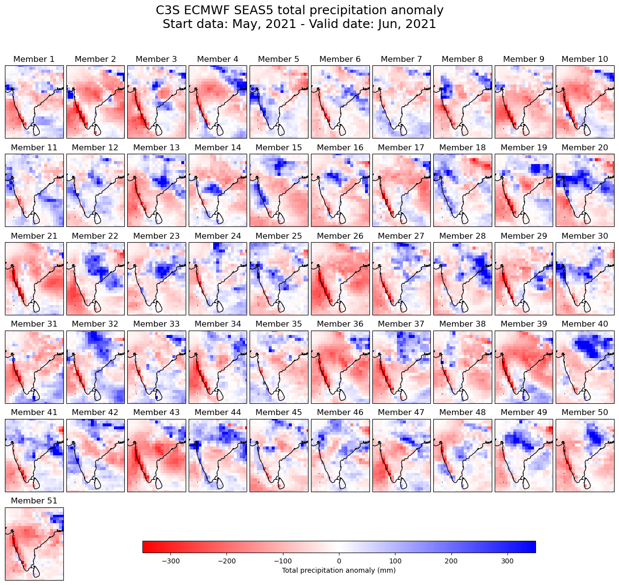
4.1 Spatial map visualization#

Now we can create a spatial map visualisation which shows for a given lead time the total precipitation anomaly of the 51 ensemble members.

# Select a leadtime to visualise
lead_time = 2

The plotting code below can be split into the following sections:

Define the overall figure: Including the size and spacing between subplots.

Create the plots: Loop over each subplot and set a customized title, add coastlines and set geographical extent.

Create a colour bar: Add a colour bar with a label.

Save the figure: Save the figure as a png file.

# Define figure and spacing between subplots
fig = plt.figure(figsize=(16, 12))
plt.subplots_adjust(hspace=0.15, wspace = 0.05)

new_date_format = seas5_SAsia['valid_time'].dt.strftime('%b, %Y')

# Define overall title
plt.suptitle('C3S ECMWF SEAS5 total precipitation anomaly'
             + os.linesep + 
             f'Start data: {str(new_date_format[0].data)}' 
             + f' - Valid date: {str(new_date_format[lead_time-1].data)}'
             , fontsize=18)

# Define each subplot looping through the ensemble members
for n in np.arange(51):
    # Add a new subplot iteratively
    ax = plt.subplot(6, 10, n + 1, projection=ccrs.PlateCarree())
    # Plot data
    im = ax.pcolormesh(seas5_SAsia.longitude.values, seas5_SAsia.latitude.values, 
                       seas5_SAsia[n,lead_time-1,:,:], cmap='bwr_r', vmin=-350, vmax=350)
    ax.set_title(f'Member {n+1}') # Set subplot title
    ax.coastlines(color='black') # Add coastlines
    # Set the extent (x0, x1, y0, y1) of the map in the given coordinate system.
    ax.set_extent([sub[1],sub[3],sub[2],sub[0]], crs=ccrs.PlateCarree())

# Create a colour bar at the bottom of the fugure
fig.subplots_adjust(bottom=0.0)
# Add axis to make space for colour bar (left, bottom, width, height)
cbar_ax = fig.add_axes([0.3, 0.05, 0.5, 0.02])
fig.colorbar(im, cax=cbar_ax, orientation='horizontal', label='Total precipitation anomaly (mm)')

# Save the figure
fig.savefig('{}/TotalPrecAnomalyForecastSAsia.png'.format(DATADIR) )

_images/445b47071201175bf2176e765cd242527a146a359961d5c0046f165109e3cace.png

4.2 Plot of total precipitation anomalies for each seasonal forecast month#

In this step we will summarise the total precipitation behaviour over the whole region for each lead time month. We will do this by averaging in the spatial (latitude and longitude) dimensions.

To put the anomalies in context they will be compared to the reference climate computed in this subregion from the hindcast data.

Conversion of data into two dimensional pivot table#

To facilitate further processing we will convert the data array into a pandas.Dataframe object with the function to_dataframe(). Pandas dataframes are optimised for the processing and visualisation of two dimensional data. We may want to drop coordinates that are not needed. We can do this with the function drop_vars().

anoms_SAsia_df = anoms_SAsia.drop_vars(['time','surface','numdays']).to_dataframe(name='anomaly')
anoms_SAsia_df

		valid_time	anomaly
number	forecastMonth
0	1	2021-05-01	97.454814
	2	2021-06-01	-12.441003
	3	2021-07-01	-35.019983
	4	2021-08-01	32.088538
	5	2021-09-01	49.202113
...	...	...	...
50	2	2021-06-01	-51.997631
	3	2021-07-01	-28.854360
	4	2021-08-01	-1.435282
	5	2021-09-01	-2.669517
	6	2021-10-01	10.027836

306 rows × 2 columns

We will now reorganise the data structure to facilitate plotting. We will do this through the use of the following Pandas functions:

reset_index().drop(): We use reset_index() to convert the ensemble members into columns, and we use drop() to remove the forecastMonth column, as we have the same information in the valid_time dimension
set_index(): allows us to define which column(s) shall be used as data frame indices
unstack(): converts the columns into a pivot table, thus re-arranging the data into an easily manageable two dimensional table.

anoms_SAsia_df = anoms_SAsia_df.reset_index().drop('forecastMonth',axis=1).set_index(['valid_time','number']).unstack()
anoms_SAsia_df

	anomaly
number	0	1	2	3	4	5	6	7	8	9	...	41	42	43	44	45	46	47	48	49	50
valid_time
2021-05-01	97.454814	42.992259	82.841835	83.515720	29.243417	50.775023	44.794726	43.992594	25.161859	48.833183	...	59.903169	75.798983	39.102171	113.692666	108.817150	97.771381	46.071874	75.845758	92.304777	86.245691
2021-06-01	-12.441003	-66.324112	-38.459383	-12.439766	1.831797	-11.853113	1.126946	-15.370852	-60.613205	-50.836803	...	21.439718	-75.826230	35.256274	-11.946277	13.234969	-20.912629	-14.152486	8.638822	-27.741443	-51.997631
2021-07-01	-35.019983	58.946688	-2.905542	-1.604468	-19.903844	-29.689120	64.252113	-26.614394	-27.099666	40.771439	...	51.486498	25.997243	-26.168625	62.856923	-0.193943	-19.738835	-23.999144	6.595067	-13.070137	-28.854360
2021-08-01	32.088538	0.594892	41.312095	10.145496	18.510533	31.572193	8.247066	25.004536	-32.636729	18.872920	...	-19.144025	19.974010	8.541381	-37.129632	-66.371737	32.188548	16.208042	-11.574989	3.477898	-1.435282
2021-09-01	49.202113	53.090658	-30.045500	-22.637873	43.004068	-0.990100	18.410411	31.951699	28.575288	-6.805420	...	29.403535	-17.086590	6.541905	55.670577	-39.139575	30.141381	-5.011032	49.144603	-52.868572	-2.669517
2021-10-01	75.735202	33.170147	-6.718222	-56.326062	-53.536046	30.948807	29.024350	10.704455	-39.323099	47.989398	...	53.165639	-21.611440	28.078094	60.934471	-3.091960	-24.675772	-62.405465	67.251144	-30.673555	10.027836

6 rows × 51 columns

The data frame above provides us for each ensemble member and forecast month the total precipitation anomaly.

As a last step, to improve the labels of our data plot later on, we will convert the valid_time column values from YYYY-MM-DD format into Month, Year format.

anoms_SAsia_m_yr = anoms_SAsia_df.reset_index()
anoms_SAsia_m_yr['valid_time'] = anoms_SAsia_m_yr['valid_time'].dt.strftime('%b, %Y')

Repeat steps for hindcast data (to compare forecast and hindcast anomalies)#

We would like now to repeat the steps for the hindcast data in order to show the forecast in the context of the reference climate. I.e. we will compare the seasonal forecast and hindcast anomalies for each lead-time month. In the final plot we will show the anomaly of each forecast ensemble member, while the model climate defined by the hindcasts will be represented in the form of tercile categories. This will put each ensemble member forecast anomaly into context and will give us an indication of its intensity.

We therefore revisit the hindcast data (tprate_hindcast), which we loaded in section 2 above. We will apply the same steps to create a geographical subset and aggregate spatially.

tprate_hindcast_SAsia = ds_latlon_subset(tprate_hindcast, sub)

To create the weighted average of the two dimensions latitude and longitude, we can use the same weights as above.

tprate_hindcast_SAsia = tprate_hindcast_SAsia.weighted(weights).mean(['latitude','longitude'])

The resulting array has three remaining dimensions, number, forecastMonth and time.

The next step is to compute the hindcast anomalies using the hindcast climatology as reference. As before, we create the hindcast climatology by computing the mean over the two dimensions number (ensemble member) and time (years) resulting in the climatology for each lead-time month. We then subtract this from the hindcast data to derive the anomalies.

anom_hindcast = tprate_hindcast_SAsia - tprate_hindcast_SAsia.mean(['number','time'])

We now repeat the same steps to convert precipitation accumulations in m/s to total precipitation in m.

valid_time = [ pd.to_datetime(anom_hindcast.time.values[0]) + relativedelta(months=fcmonth-1) for fcmonth in anom_hindcast.forecastMonth]
numdays = [monthrange(dd.year,dd.month)[1] for dd in valid_time]
anom_hindcast = anom_hindcast.assign_coords(numdays=('forecastMonth',numdays))

anom_hindcast_tp = anom_hindcast * anom_hindcast.numdays * 24 * 60 * 60 * 1000

Calculation of hindcast anomaly terciles#

Now, for each of the lead-time months, we can compute the minimum and maximum as well as the 1/3 and 2/3 percentiles of the hindcast anomaly ensemble.

P0 = anom_hindcast_tp.min(['number','time'])
P33 = anom_hindcast_tp.quantile(1/3.,['number','time'])
P66 = anom_hindcast_tp.quantile(2/3.,['number','time'])
P100 = anom_hindcast_tp.max(['number','time'])

A last step before we visualise this data is to

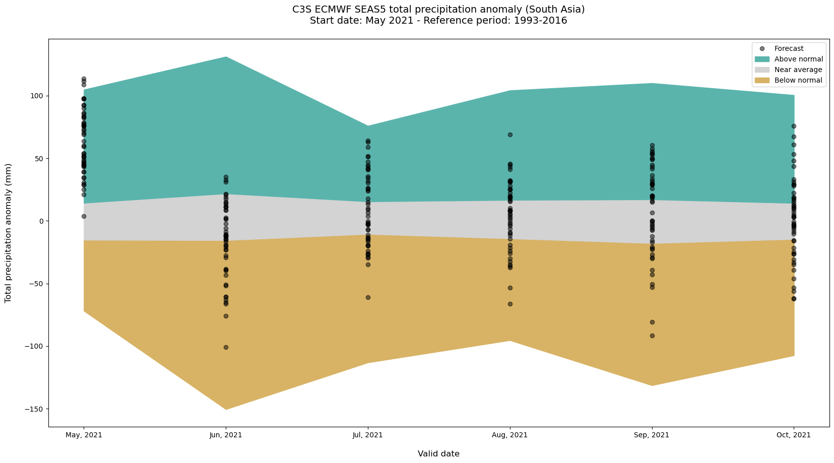
The last step is to visualize the hindcast climatology boundaries as filled area and the ensemble seasonal forecast anomalies for each forecast month. The visualisation code below has three main sections:

Initiate the figure: Initiate a matplotlib figure

Plot the seasonal forecast anomalies + climatology boundaries: Plot the ensemble seasonal forecast anomalies as black circles and the hindcast climatology as filled areas

Customise plot settings: Add additonal features, such as title, x- and y-axis labels etc.

# Initiate the figure
fig=plt.figure(figsize=(20, 10))
ax=fig.gca()

# Plot the seasonal forecast anomalies + climatology boundaries as filled areas
ax.plot(anoms_SAsia_m_yr.valid_time, anoms_SAsia_m_yr.anomaly, marker='o', linestyle='', color='black', alpha=0.5, label='Forecast')
ax.fill_between(anoms_SAsia_m_yr.index,P66,P100,color='#5ab4ac',label='Above normal')
ax.fill_between(anoms_SAsia_m_yr.index,P33,P66,color='lightgray',label='Near average')
ax.fill_between(anoms_SAsia_m_yr.index,P0,P33,color='#d8b365',label='Below normal')

# Customize plot settings
plt.title('C3S ECMWF SEAS5 total precipitation anomaly (South Asia)' 
          + os.linesep + 
          'Start date: May 2021 - Reference period: 1993-2016' 
          + os.linesep, fontsize=14)

handles, labels = plt.gca().get_legend_handles_labels()
by_label = OrderedDict(zip(labels, handles))
plt.legend(by_label.values(), by_label.keys())

ax.set_ylabel('Total precipitation anomaly (mm)' + os.linesep, fontsize=12)
ax.set_xlabel(os.linesep + 'Valid date', fontsize=12)

# Save the figure
fig.savefig('{}/TotalPrecForecastHindcastAnomaliesSAsia.png'.format(DATADIR) )

_images/39ddd776716145cc7d5eab5357a709d0622180e9d95930d86bff08b3be2847ac.png

5. Calculate seasonal forecast 3-month anomalies#

In this last section of the tutorial we will show how to create plots similar to those on the Copernicus Climate Change Service (C3S) website. This process includes calculating 3-month aggregations and ensemble means. This differs from the previous sections where we have focussed on the processing of monthly data and individual members.

Compute 3-month rolling averages#

The first step is to compute 3-month rolling averaged for the seasonal forecasts and hindcast data. We will do this through a combination of the xarray functions rolling() and mean().

seas5_forecast_3m = seas5_forecast.rolling(forecastMonth=3).mean()
ds_hindcast_3m = ds_hindcast.rolling(forecastMonth=3).mean()

Calculate anomalies#

We now repeat the process of calculating anomalies with respect to the climatology, this time for the 3-monthly data.

ds_hindcast_3m_hindcast_mean = ds_hindcast_3m.mean(['number','time'])
seas5_anomalies_3m_202105 = seas5_forecast_3m.tprate - ds_hindcast_3m_hindcast_mean.tprate

Ensemble mean anomaly#

We want to compute the average of the 3-month seasonal forecast anomaly of the ensemble members. For this, we have to average over the dimension number. The final array has three dimensions, forecastMonth, latitude and longitude.

seas5_anomalies_3m_202105_em = seas5_anomalies_3m_202105.mean('number')

Convert precipitation rate to accumulation in mm#

The last step before visualizing the 3-month seasonal forecast anomalies is again to convert the precipitation accumulations to total precipitation in mm. We repeat the same steps as previously:

Calculate number of days for each forecast month and add it as coordinate info

Name the 3-month rolling archives to indicate over which months the average was built

Convert the precipitation accumulations based on the number of days

Add updated attributes to the data array

# Calculate number of days for each forecast month and add it as coordinate information to the data array
vt = [ pd.to_datetime(seas5_anomalies_3m_202105_em.time.values) + relativedelta(months=fcmonth-1) for fcmonth in seas5_anomalies_3m_202105_em.forecastMonth]
vts = [[thisvt+relativedelta(months=-mm) for mm in range(3)] for thisvt in vt]
numdays = [np.sum([monthrange(dd.year,dd.month)[1] for dd in d3]) for d3 in vts]
seas5_anomalies_3m_202105_em = seas5_anomalies_3m_202105_em.assign_coords(numdays=('forecastMonth',numdays))

# Define names for the 3-month rolling archives, that give an indication over which months the average was built
vts_names = ['{}{}{} {}'.format(d3[2].strftime('%b')[0],d3[1].strftime('%b')[0],d3[0].strftime('%b')[0], d3[0].strftime('%Y'))  for d3 in vts]
seas5_anomalies_3m_202105_em = seas5_anomalies_3m_202105_em.assign_coords(valid_time=('forecastMonth',vts_names))
seas5_anomalies_3m_202105_em

# Convert the precipitation accumulations based on the number of days
seas5_anomalies_3m_202105_em_tp = seas5_anomalies_3m_202105_em * seas5_anomalies_3m_202105_em.numdays * 24 * 60 * 60 * 1000

# Add updated attributes
seas5_anomalies_3m_202105_em_tp.attrs['units'] = 'mm'
seas5_anomalies_3m_202105_em_tp.attrs['long_name'] = 'SEAS5 3-monthly total precipitation ensemble mean anomaly for 6 lead-time months, start date in May 2021.'

Visualise 3-monthly total precipitation ensemble mean anomalies#

Let us now visualise the 3-month total precipitation ensemble mean anomaly in an interactive plot. Widgets (ipywidgets) allow us to add interactive features to Jupyter notebooks. We will use these to add a dropdown menu that offers the option to choose the 3-monthly periods over which the anomalies are averaged. Given that we have 6 lead-time months, we end up with only 4 possible 3-monthly periods (the last 2 months are insufficient to create a complete 3-month aggregation).

vts_names

['MAM 2021', 'AMJ 2021', 'MJJ 2021', 'JJA 2021', 'JAS 2021', 'ASO 2021']

dropdown_opts = [(vts_names[mm-1],mm) for mm in range(3,7)]

tp_colors = [(153/255.,51/255.,0),(204/255.,136/255.,0),(1,213/255.,0),
             (1,238/255.,153/255.),(1,1,1),(204/255.,1,102/255.),
             (42/255.,1,0),(0,153/255.,51/255.),(0,102/255.,102/255.)]  
tp_levels = [-200,-100,-50,-10,10,50,100,200]



def plot_leadt(ds, leadt_end):
    array = ds.sel(forecastMonth=leadt_end)
    fig, ax = plt.subplots(1, 1, figsize = (16, 8), subplot_kw={'projection': ccrs.PlateCarree()})
    im = plt.contourf(array.longitude, array.latitude, array, 
                      levels=tp_levels, colors=tp_colors, extend='both')
    ax.set_title(f'{array.long_name}' + os.linesep + f'{array.valid_time.values}', fontsize=16)
    ax.gridlines(draw_labels=True, linewidth=1, color='gray', alpha=0.5, linestyle='--') 
    ax.coastlines(color='black')
    cbar = plt.colorbar(im,fraction=0.05, pad=0.04)
    cbar.set_label(array.units)
    
    return
    
dropdown_opts = [(vts_names[mm-1],mm) for mm in range(3,7)] 
a=widgets.interact(plot_leadt, ds=widgets.fixed(seas5_anomalies_3m_202105_em_tp), 
                   leadt_end=widgets.Dropdown(options=dropdown_opts,description='Valid Time:', 
                                              style={'description_width': 'initial'}))

NOTE:
The plots shown here are similar but not identical to those on the Copernicus Climate Change Service (C3S) website, specifically here. These plots are not identical however. The white areas in both plots, for example, have different meanings: those on the C3S website have a significance test to white-out non statistically-significant anomalies.

This project is licensed under APACHE License 2.0. | View on GitHub

Seasonal Forecast Anomalies

Contents

Seasonal Forecast Anomalies#

About#

Install packages#

Load packages#

1. Request data from the CDS programmatically with the CDS API#

2. Calculate seasonal hindcast climate mean#

Read the downloaded data#

Change representation of forecast lead time#

Extract data array from dataset#

Average over ensemble members and years to create hindcast climatology#

3. Load monthly seasonal forecast data for 2021 and calculate seasonal forecast anomalies#

Load seasonal forecast data for 2021 and change representation of forecast lead time#

Calculate 2021 anomalies#

Convert forecast lead time month into dates#

Convert from precipitation rates to accumulation#