CORDEX biases in the SPEI6 drought index over the Mediterranean region

5.2.7. CORDEX biases in the SPEI6 drought index over the Mediterranean region#

Production date: 17-03-2026

Produced by: CMCC foundation - Euro-Mediterranean Center on Climate Change. Albert Martinez Boti and Lorenzo Sangelantoni.

🌍 Use case: Calculating drought indices from climate projections data to inform water management#

❓ Quality assessment question#

How well do CORDEX models simulate drought compared to signals derived from ERA5?

The Standardized Precipitation-Evapotranspiration Index (SPEI) [1] is a widely used drought indicator that integrates precipitation and potential evapotranspiration, providing a more complete measure of water deficits than precipitation alone. Its multiscalar formulation allows the evaluation of different types of drought [2], from short-term agricultural or soil moisture deficits to long-term hydrological or ecological events. Being standardised, SPEI is dimensionless, facilitating comparisons across regions and climates. By capturing variations in frequency, duration, and severity, it effectively reflects the complex nature of drought, making it a robust and physically meaningful proxy for drought assessment in the context of climate change [3].

Understanding SPEI is particularly relevant for the water management sector. By capturing multiple types of drought SPEI serves as a versatile indicator for various users. Climate projections using SPEI enable planners to anticipate future water deficits, guide allocation, and design effective strategies for reservoir management, irrigation, and drought preparedness, helping to reduce socio-economic and ecological impacts [4][5].

This assessment evaluates SPEI6 (six-month accumulation) across a subset of CORDEX models available through the Copernicus Climate Data Store (CDS). Model outputs are compared against SPEI6 derived from ERA5 reanalysis, which serves as the reference product. We specifically evaluate whether changes in the 1991–2010 period relative to the 1971–1990 baseline are accurately represented by CORDEX models and the trend across the whole 1971-2010 period for the Mediterranean domain.

This notebook is the counterpart to the assessment performed for CMIP6 (CMIP6 biases in the SPEI6 drought index over the Mediterranean region)

📢 Quality assessment statement#

These are the key outcomes of this assessment

The CORDEX ensemble median for the subset of models considered in this assessment does not generally capture the general intensification of drought over the Mediterranean observed in ERA5, showing SPEI6 changes close to zero for most regions.
Individual models exhibit highly diverse spatial patterns, with some closely resembling ERA5, underscoring the importance of taking into account the whole ensemble (and not only the ensemble mean) for planning purposes.
Despite these biases, the selected subset of CORDEX models may still be useful for exploring SPEI-based future water deficits and guiding drought preparedness, as long as limitations are considered.
Regions with high inter-model spread, such as North Africa, Turkey, and the eastern Mediterranean, may be associated with future higher uncertainty, suggesting that adaptation strategies in these areas should consider a wider range of possible futures.

Visual abstract — Fig. 5.2.7.1 Spatial patterns of SPEI6 change over the Mediterranean region. Panels show (a) ERA5 reference, (b) CORDEX ensemble median (median of the selected subset of models at each grid cell), (c) ensemble median bias relative to ERA5, and (d) ensemble spread (standard deviation across the selected models). SPEI6 is standardised over the reference period 1971–2010. SPEI6 change is calculated at each grid point as the difference between the monthly climatologies of the target period (1991–2010) and the baseline period (1971–1990), and then averaged to obtain the ANNUAL mean.#

📋 Methodology#

The Standardized Precipitation-Evapotranspiration Index accumulated to six months (SPEI6) has been calculated for this assessment — through the use of xclim — as a proxy to evaluate drought conditions for a subset of CORDEX models, which are evaluated against SPEI6 derived from ERA5 reanalysis. The study covers the Mediterranean domain, following IPCC-AR6 regional definitions [6], and results include spatial maps of SPEI6 changes for ERA5, CORDEX, and the biases of these changes. Additionally, time series showing the temporal evolution of drought across the domain are calculated, comparing trends from the models with ERA5 over the historical period considered within this assessment (1971–2010).

Potential evapotranspiration (PET) is calculated with the Hargreaves method [7], which requires only maximum and minimum temperature (and optionally mean temperature), providing a computationally efficient yet robust estimate (e.g., [8]). The accumulated series of precipitation minus PET is then standardised for the reference period, defined by the C3S Atlas (1971–2010).

Five key concepts are defined:

Reference period: The period used to standardise SPEI values, here 1971–2010, following the C3S Atlas.
Baseline period: The period against which changes are calculated, here 1971–1990.
Target period: The period for which changes are evaluated, here 1991–2010.
Historical period: The entire period considered in this assessment, here 1971–2010.
SPEI6 change: Differences in SPEI6 between the target period and the baseline, representing anomalies in drought conditions.

The analysis and results follow the next outline:

1. Parameters, requests and functions definition

1.1. Import packages
1.2. Define Parameters
1.3. Define models
1.4. Define ERA5 request
1.5. Define model requests
1.6. Functions to cache

2. Downloading and processing

2.1. Download and transform ERA5
2.2. Download and transform models
2.3. Apply land-sea mask and change some attributes

3. Plot and describe results

3.1. Define plotting functions
3.2. Plot ensemble maps
3.3. Plot ensemble maps - Seasonal aggregations
3.4. Plot model maps
3.5. Plot bias maps
3.6. Timeseries
3.7. Results summary
3.8. Implications for the users

NOTE ON THE METHODOLOGY:
This notebook follows the same methodology as the assessment performed for CMIP6 ( CMIP6 biases in the SPEI6 drought index over the Mediterranean region). The historical period considered here is slightly shorter (1971–2010) compared to 1961–2020 in the CMIP6 assessment. This choice helps to avoid memory overload, ensures efficient execution of the notebook, guarantees availability of CORDEX models for the historical period, and avoids including many years of scenario data (CORDEX historical runs only extend until 2005).

📈 Analysis and results#

1. Parameters, requests and functions definition#

1.1. Import packages#

1.2. Define Parameters#

In the “Define Parameters” section, various customisable options for the notebook are specified:

The historical period can be adjusted by modifying historical_slice; the default range is 1971-2010.
The reference period can be adjusted by modifying reference_slice; the default range is 1971–2010, following the C3S Atlas.
The baseline period can be adjusted by modifying baseline_slice; the default range is 1971-1990.
The target period can be adjusted by modifying target_slice; the default range is 1991-2010.
The interpolation_method parameter allows selecting the interpolation method when regridding is performed.
collection_id is not customisable for this assessment and is set to ‘CORDEX’.
The area parameter specifies the geographical domain of interest. By default, the Mediterranean domain is used, following IPCC-AR6 regional definitions [6]
The time_agg allows selecting the time aggregation for the analysis. Options include: annual, DJF, MAM, JJA, SON, Jan, Feb, Mar, Apr, May, Jun, Jul, Aug, Sep, Oct, Nov, Dec.
SPEI accumulation window (window): Defines the accumulation period in months for the SPEI calculation. Common options include 3, 6, or 12 months, depending on whether short-term or long-term droughts are of interest. In this assessment, a six-month accumulation is used.
The chunks selection allows the user to define if dividing into chunks when downloading the data on their local machine. Although it does not significantly affect the analysis, it is recommended to keep the default value for optimal performance.

1.3. Define models#

The following climate analyses are performed using a subset of CORDEX models that provide both the historical and RCP8.5 experiments, as well as maximum, minimum and mean temperature and precipitation, within the Climate Data Store (CDS). All Global Climate Models (GCMs) driving the selected CORDEX simulations were included, and the selection ensures a representative coverage of the available Regional Climate Models (RCMs). A total of 17 models were chosen to maintain consistency with the number used in the quality assessment CMIP6 biases in the SPEI6 drought index over the Mediterranean region.

1.4. Define ERA5 request#

Within this notebook, ERA5 serves as the reference product. In this section, we set the required parameters for the cds-api data-request of ERA5.

1.5. Define model requests#

In this section we set the required parameters for the cds-api data-request.

Show code cell source

Hide code cell source

request_cordex = {
    "format": "zip",
    "domain": "europe",
    #"experiment": "historical",
    "horizontal_resolution": "0_11_degree_x_0_11_degree",
    "temporal_resolution": "daily_mean",
    "variable": [
        "2m_air_temperature",
        "maximum_2m_temperature_in_the_last_24_hours",
        "minimum_2m_temperature_in_the_last_24_hours",
        "mean_precipitation_flux"
    ],
    "ensemble_member": "r1i1p1",
}


def get_cordex_years(
    year_start,
    year_stop,
    start_years=list(range(1951, 2097, 5)),
    end_years=list(range(1955, 2101, 5)),
):
    start_year = []
    end_year = []
    years = set(range(year_start, year_stop + 1))
    for start, end in zip(start_years, end_years):
        if years & set(range(start, end + 1)):
            start_year.append(start)
            end_year.append(end)
    return start_year, end_year



model_requests = {}
if collection_id == "CORDEX":
    for gcm_model in gcm_models:
        for model in models_cordex[gcm_model]:
            # Historical (until 2005)
            if historical_slice.stop <= 2005:
                # Only historical
                start_years = list(range(historical_slice.start, historical_slice.stop + 1, 5))
                end_years = list(range(historical_slice.start + 4, historical_slice.stop + 5, 5))
                requests = [
                    {
                        "rcm_model": model,
                        "gcm_model": gcm_model,
                        **request_cordex,
                        "experiment": "historical",
                        "start_year": [str(start_year)],
                        "end_year": [str(end_year)],
                    }
                    for start_year, end_year in zip(
                        *get_cordex_years(
                            historical_slice.start,
                            historical_slice.stop,
                            start_years=start_years,
                            end_years=end_years,
                        )
                    )
                ]
            elif historical_slice.stop > 2005:
                # Historical part (until 2005)
                start_years_hist = list(range(historical_slice.start, 2006, 5))
                end_years_hist = list(range(historical_slice.start + 4, 2010, 5))
                requests = [
                    {
                        "rcm_model": model,
                        "gcm_model": gcm_model,
                        **request_cordex,
                        "experiment": "historical",
                        "start_year": [str(start_year)],
                        "end_year": [str(end_year)],
                    }
                    for start_year, end_year in zip(
                        *get_cordex_years(
                            historical_slice.start,
                            2005,
                            start_years=start_years_hist,
                            end_years=end_years_hist,
                        )
                    )
                ]

                # Future part (RCP8.5 from 2006 onwards)
                start_years_fut = list(range(2006, historical_slice.stop + 1, 5))
                end_years_fut = list(range(2010, historical_slice.stop + 5, 5))
                requests += [
                    {
                        "rcm_model": model,
                        "gcm_model": gcm_model,
                        **request_cordex,
                        "experiment": "rcp_8_5",
                        "start_year": [str(start_year)],
                        "end_year": [str(end_year)],
                    }
                    for start_year, end_year in zip(
                        *get_cordex_years(
                            2006,
                            historical_slice.stop,
                            start_years=start_years_fut,
                            end_years=end_years_fut,
                        )
                    )
                ]
            else:
                requests = []

            model_requests[f"{gcm_model}_{model}"] = (
                "projections-cordex-domains-single-levels",
                requests,
            )
else:
    raise NotImplementedError

1.6. Functions to cache#

In this section, functions that will be executed in the caching phase are defined. Caching is the process of storing copies of files in a temporary storage location, so that they can be accessed more quickly. This process also checks if the user has already downloaded a file, avoiding redundant downloads.

Description of the main functions:

compute_spei_cordex: Uses the xclim package to calculate the Standardized Precipitation-Evapotranspiration Index (SPEI). The reference_slice argument specifies the reference period used for standardization, while the window argument defines the number of months over which precipitation and evapotranspiration are accumulated (6 months in this assessment).
get_mask_below_03: Generates a mask identifying grid points where precipitation is below 0.3 mm/day, allowing filtering of extremely dry regions.

Show code cell source

Hide code cell source

def add_bounds(ds):
    for coord in {"latitude", "longitude"} - set(ds.cf.bounds):
        ds = ds.cf.add_bounds(coord)
    return ds


def get_grid_out(request_grid_out, method):
    ds_regrid = download.download_and_transform(*request_grid_out)
    coords = ["latitude", "longitude"]
    if method == "conservative":
        ds_regrid = add_bounds(ds_regrid)
        for coord in list(coords):
            coords.extend(ds_regrid.cf.bounds[coord])
    grid_out = ds_regrid[coords]
    coords_to_drop = set(grid_out.coords) - set(coords) - set(grid_out.dims)
    grid_out = ds_regrid[coords].reset_coords(coords_to_drop, drop=True)
    grid_out.attrs = {}
    return grid_out

def compute_spei_cordex(ds,
                        reference_slice,
                        window=6,
                        resample_reduction=False,
                        request_grid_out = None,
                        area=None,
                        **regrid_kwargs
                       ):


    ds=ds.convert_calendar('proleptic_gregorian', align_on='date', use_cftime=False)
    # Cutout
    if area:
        regionalise_kwargs = {
            "lon_slice": slice(area[1], area[3]),
            "lat_slice": slice(area[0], area[2]),
        }
        ds = utils.regionalise(ds, **regionalise_kwargs)

    # Original bounds for conservative interpolation
    if regrid_kwargs.get("method") == "conservative":
        regrid_kwargs.setdefault("ignore_degenerate", True)
        ds = add_bounds(ds)
        bounds = [
                ds.cf.get_bounds(coord).reset_coords(drop=True)
                for coord in ("latitude", "longitude")
            ]
    else:
        bounds = []

    if request_grid_out:
        # Rechunk spatial dimensions to a single chunk for xESMF / apply_ufunc
        spatial_dims = [
            dim for dim in ds.dims
            if dim.lower() in {"lon","longitude","x","i","rlon","lat","latitude","y","j","rlat"}
        ]

        if spatial_dims:
            ds = ds.chunk(-1) 

        # Ensure variables are numeric for xESMF
        for v in ds.data_vars:
            if ds[v].dtype == "object":
                ds[v] = ds[v].astype("float64")

        ds = diagnostics.regrid(
                ds,
                grid_out=get_grid_out(request_grid_out, regrid_kwargs["method"]),
                **regrid_kwargs,
        )

    if resample_reduction:
        # Apply correct daily reductions
        pr = ds["tp"].resample(time="1D").sum(keep_attrs=True)* 1000
        tas = ds["t2m"].resample(time="1D").mean(keep_attrs=True)
        tasmax = ds["t2m"].resample(time="1D").max(keep_attrs=True)
        tasmin = ds["t2m"].resample(time="1D").min(keep_attrs=True)
        pr.attrs["units"] = "mm/day"
    else:
        pr = ds["pr"] * 86400
        pr.attrs["units"] = "mm/day"


    
    da_pet=xclim.indices.potential_evapotranspiration(tas = tas if resample_reduction else ds["tas"],
                                                      tasmin = tasmin if resample_reduction else ds["tasmin"],
                                                      tasmax = tasmax if resample_reduction else ds["tasmax"],
                                                      method='HG85')*86400
    da_pet.attrs["units"] = "mm/day"

    wb = pr - da_pet
    wb.attrs["units"] = "mm/day"
    wb = wb.convert_calendar("proleptic_gregorian", align_on="date", use_cftime=False)
    
    da_spei = xclim.indices.standardized_precipitation_evapotranspiration_index(wb,
                                                                                freq='MS',
                                                                                window=window,
                                                                                cal_start=f"{reference_slice.start}-01-01",
                                                                                cal_end=f"{reference_slice.stop}-12-31")
    # Wrap into dataset
    ds_out = xr.Dataset({"spei": da_spei})
    ds_out["spei"].attrs = da_spei.attrs

    return ds_out



    


def get_mask_below_03(ds,threshold,resample_reduction=True):
    # Select pr         
    if resample_reduction:
        # Apply correct daily reductions
        pr = ds["tp"].resample(time="1D").sum(keep_attrs=True)* 1000   
        pr.attrs["units"] = "mm/day"
        pr_mean =pr.mean(dim = 'time')
        pr_mask = 1 - xr.where(pr_mean<threshold, 1, 0)
        ds_out = xr.Dataset({"pr_mask": pr_mask})
    return ds_out

2. Downloading and processing#

2.1. Download and transform ERA5#

In this section, the download.download_and_transform function from the ‘c3s_eqc_automatic_quality_control’ package is used to retrieve ERA5 hourly reference data, resample it to daily frequency, compute daily potential evapotranspiration, calculate the daily water balance, and derive the SPEI (SPEI6 for this assessment). Results are cached to avoid redundant downloads and repeated processing.

2.2. Download and transform models#

In this section, the download.download_and_transform function from the ‘c3s_eqc_automatic_quality_control’ package is used to download daily data from CORDEX models, compute daily potential evapotranspiration, calculate the daily water balance, and derive the SPEI (SPEI6 for this assessment). SPEI6 is computed on each model’s native grid and also on the ERA5 grid to enable bias assessment. When regridding is required, it is performed for each essential climate variable before the index calculation to preserve standardisation. Results are cached to avoid redundant downloads and repeated processing.

model='cccma_canesm2_clmcom_clm_cclm4_8_17'
model='cccma_canesm2_gerics_remo2015'
model='cnrm_cerfacs_cm5_ipsl_wrf381p'
model='cnrm_cerfacs_cm5_smhi_rca4'
model='ichec_ec_earth_dmi_hirham5'
model='ichec_ec_earth_knmi_racmo22e'
model='ipsl_cm5a_mr_ipsl_wrf381p'
model='ipsl_cm5a_mr_knmi_racmo22e'
model='miroc_miroc5_clmcom_clm_cclm4_8_17'
model='miroc_miroc5_gerics_remo2015'
model='mohc_hadgem2_es_cnrm_aladin63'
model='mohc_hadgem2_es_mohc_hadrem3_ga7_05'
model='mpi_m_mpi_esm_lr_mpi_csc_remo2009'
model='mpi_m_mpi_esm_lr_cnrm_aladin63'
model='ncc_noresm1_m_dmi_hirham5'
model='ncc_noresm1_m_mohc_hadrem3_ga7_05'
model='ncc_noresm1_m_smhi_rca4'

2.3. Apply land-sea mask and change some attributes#

This section changes some attributes and applies a land–sea mask to all models, as well as to ERA5. A bare-earth (barrean) mask is also applied to ensure meaningful results in arid regions, as in the C3S atlas. In particular, we follow the methodology available in their Github repository. While their implementation of the mask also considers factors such as snow depth and vegetation cover, here we only apply the filter based on annual mean precipitation for 1971–2010 being less than 0.3 mm day⁻¹. This simplification is justified because, in the region under consideration, the bare-earth mask obtained with the full set of filters closely matches the one derived from the precipitation threshold alone.

Note: ds_interpolated contains data from the models regridded to the ERA5 grid. model_datasets contain the same data on the original grid of each model. Regridding is performed for every essential climate variable prior to the index calculation in order to avoid compromising standardisation.

100%|██████████| 1/1 [00:00<00:00, 22.34it/s]

3. Plot and describe results#

This section will display the following results:

SPEI6 change maps comparing ERA5 and the ensemble median (defined as the median of the change values for the selected subset of models at each grid cell). The layout includes ERA5, the ensemble median, the ensemble median bias, and the ensemble spread (calculated as the standard deviation of the change across the selected subset of models).
SPEI6 change maps for each individual model.
Bias maps of the SPEI6 change for each model.
Time series of SPEI6 change (averaged over the Mediterranean region).

Note: SPEI6 change is calculated at each grid point as the arithmetic difference between climatologies in the target period (1991–2010) and the baseline period (1971–1990).

3.1. Define plotting functions#

The functions presented here are used to calculate SPEI6 changes and generate corresponding layout plots. Three types of layout can be displayed, depending on the plotting function:

Reference and ensemble summary: Includes the ERA5 reference product, the ensemble median, the bias of the ensemble median, and the ensemble spread. This is generated using plot_ensemble().
Individual models: Displays all models individually using plot_models().
Model biases: Displays the bias of each model relative to the reference, also using plot_models().

Calculation of SPEI6 change:

compute_spei_change() calculates SPEI6 change at each grid point as the arithmetic difference between monthly climatologies of the target period (1991–2010) and the baseline period (1971–1990). It then aggregates the change according to the user-specified time_agg in Section 1.2.
compute_change_4timeseries() computes SPEI6 anomalies relative to the baseline climatology for each month of the timeseries and aggregates them according to the time_agg parameter. This provides monthly, seasonal, or annual-level information depending on the user’s selection.

Show code cell source

Hide code cell source

def compute_spei_change(ds, baseline_slice, target_slice, time_agg="annual"):
    # Mapping months to names
    month_map = {
        "Jan": [1], "Feb": [2], "Mar": [3], "Apr": [4],"May": [5], "Jun": [6],
        "Jul": [7], "Aug": [8],"Sep": [9], "Oct": [10], "Nov": [11], "Dec": [12]}

    # Mapping seasons to months
    season_map = {"DJF": [12, 1, 2],"MAM": [3, 4, 5],
                  "JJA": [6, 7, 8],"SON": [9, 10, 11]}
    
    valid_opts = ["annual"] + list(season_map.keys()) + list(month_map.keys())
    assert time_agg in valid_opts, f"Invalid option: {time_agg}"
    # Select baseline and target periods
    baseline = ds.sel(time=slice(f"{baseline_slice.start}-01", f"{baseline_slice.stop}-12"))["spei"]
    target   = ds.sel(time=slice(f"{target_slice.start}-01", f"{target_slice.stop}-12"))["spei"]
    # Monthly climatologies 
    clim_baseline = baseline.groupby("time.month").mean("time", keep_attrs=True)
    clim_target   = target.groupby("time.month").mean("time", keep_attrs=True)
    #get delta
    delta_time = clim_target - clim_baseline
    delta_time.attrs = ds["spei"].attrs  
    # Aggregate according to user choice
    if time_agg == "annual":
        result = delta_time.mean("month", keep_attrs=True)
    elif time_agg in season_map:
        result = delta_time.sel(month=season_map[time_agg]).mean("month", keep_attrs=True)
    elif time_agg in month_map:
        result = delta_time.sel(month=month_map[time_agg]).squeeze("month")
        result.attrs = ds["spei"].attrs  

    return result


def compute_change_4timeseries(ds, baseline_slice, time_agg="annual"):
    # Mapping months to names
    month_map = {
        "Jan": [1], "Feb": [2], "Mar": [3], "Apr": [4],"May": [5], "Jun": [6],
        "Jul": [7], "Aug": [8],"Sep": [9], "Oct": [10], "Nov": [11], "Dec": [12]}

    # Mapping seasons to months
    season_map = {"DJF": [12, 1, 2],"MAM": [3, 4, 5],
                  "JJA": [6, 7, 8],"SON": [9, 10, 11]}
    valid_opts = ["annual"] + list(season_map.keys()) + list(month_map.keys())
    assert time_agg in valid_opts, f"Invalid option: {time_agg}"

    # Select baseline period
    baseline = ds.sel(time=slice(f"{baseline_slice.start}-01", f"{baseline_slice.stop}-12"))["spei"]

    # Monthly climatology for the baseline
    clim_baseline = baseline.groupby("time.month").mean("time", keep_attrs=True)

    # Compute monthly anomalies relative to baseline climatology
    anomalies = ds["spei"].groupby("time.month") - clim_baseline

    # Preserve attributes
    anomalies.attrs = ds["spei"].attrs

    # Aggregate anomalies
    if time_agg == "annual":
        # Group by year
        result = anomalies.groupby("time.year").mean("time", keep_attrs=True)
    elif time_agg in season_map:
        # Select months for the season, then group by year
        sel_months = season_map[time_agg]
        season_anom = anomalies.sel(time=anomalies["time.month"].isin(sel_months))
        result = season_anom.groupby("time.year").mean("time", keep_attrs=True)
    elif time_agg in month_map:
        # Select the month, keep time as is
        result = anomalies.sel(time=anomalies["time.month"].isin(month_map[time_agg]))

    return result
    
def plot_trend(time_series, var_values, label, color):
    time_numeric = pd.to_numeric(time_series.to_series())
    slope, intercept, _, p_value, _ = linregress(time_numeric, var_values)
    trend = intercept + slope * time_numeric
    slope_per_decade = slope * 10 * (60 * 60 * 24 * 365.25 * 10**9)  # nanoseconds to decade
    plt.plot(time_series, trend, linestyle='--', color=color, label=label)
    return slope_per_decade, p_value

def set_extent(da, axs, area):
    extent = [area[i] for i in (1, 3, 2, 0)]
    extent[3] += -3 
    for ax in axs:
        # Grid
        subplotspec = ax.get_subplotspec()
        gridliners = [a for a in ax.artists if isinstance(a, Gridliner)]
        for gl in gridliners:
            gl.remove()
            gl = ax.gridlines(draw_labels=True, linestyle="--", linewidth=1, color="black", alpha=0.15)
            gl.top_labels = gl.right_labels = False
            gl.left_labels = subplotspec.is_first_col()
            gl.bottom_labels = subplotspec.is_last_row()
        # Extent
        ax.set_extent(extent)

def plot_models(
    data,
    da_for_kwargs=None,
    col_wrap=4,
    subplot_kw={"projection": ccrs.PlateCarree()},
    figsize=None,
    layout="constrained",
    area=area,
    flip_cmaps=False,
    cmap_params=None,
    gcm_models=None,         
    split_model_title=True,   
    **kwargs,
):
    if isinstance(data, dict):
        assert da_for_kwargs is not None
        model_dataarrays = data
    else:
        da_for_kwargs = da_for_kwargs or data
        model_dataarrays = dict(data.groupby("model"))

    # --- Determine colour parameters ---
    default_kwargs = {"robust": True, "extend": "both"}
    if cmap_params is None:
        kwargs = default_kwargs | kwargs
        cmap_params = xr.plot.utils._determine_cmap_params(
            da_for_kwargs.values, **kwargs
        )

    fig, axs = plt.subplots(
        *(col_wrap, math.ceil(len(model_dataarrays) / col_wrap)),
        subplot_kw=subplot_kw,
        figsize=figsize,
        layout=layout,
    )
    axs = axs.flatten()

    # --- Helper function to split GCM and RCM ---
    def format_model_title(model_name):
        if gcm_models is None:
            return model_name  # fallback
        for gcm in gcm_models:
            if model_name.startswith(gcm):
                rcm = model_name[len(gcm)+1:]  # +1 to remove underscore
                return f"{gcm}\n{rcm}"
        return model_name  # fallback if no match

    # --- Plot each model ---
    for (model, da), ax in zip(model_dataarrays.items(), axs):
        pcm = plot.projected_map(
            da, ax=ax, show_stats=False, add_colorbar=False, **cmap_params
        )

        if split_model_title:
            ax.set_title(format_model_title(model))
        else:
            ax.set_title(model)

    # --- Hide empty axes ---
    for ax in axs[len(model_dataarrays):]:
        ax.set_visible(False)

    # --- Shared extent and colourbar ---
    set_extent(da_for_kwargs, axs, area)
    fig.colorbar(
        pcm,
        ax=axs.flatten(),
        extend=cmap_params.get("extend", "both"),
        location="right",
        label=f"{da_for_kwargs.attrs.get('long_name', '')} [{da_for_kwargs.attrs.get('units', '')}]",
    )

    return fig

def plot_ensemble(
    da_models,
    da_era5=None,
    subplot_kw={"projection": ccrs.PlateCarree()},
    figsize=None,
    layout="constrained",
    cbar_kwargs=None,
    area=area,
    flip_cmaps=False,
    cmap_params_era5=None,
    cmap_params_median=None,
    cmap_params_bias=None,
    cmap_params_std=None,
    **kwargs,
):
    # Default behaviour
    default_kwargs = {"robust": True, "extend": "both"}
    if da_era5 is None and cbar_kwargs is None:
        cbar_kwargs = {"orientation": "horizontal"}

    # Create figure and axes
    fig, axs = plt.subplots(
        *(1 if da_era5 is None else 2, 2),
        subplot_kw=subplot_kw,
        figsize=figsize,
        layout=layout,
    )
    axs = axs.flatten()
    axs_iter = iter(axs)

    # --- ERA5 plot ---
    if da_era5 is not None:
        ax = next(axs_iter)
        params = cmap_params_era5 or xr.plot.utils._determine_cmap_params(
            da_era5.values, **default_kwargs
        )
        plot.projected_map(
            da_era5, ax=ax, show_stats=False, cbar_kwargs=cbar_kwargs, **params
        )
        ax.set_title("(a) ERA5")

    # --- Ensemble Median ---
    ax = next(axs_iter)
    median = da_models.median("model", keep_attrs=True)
    params = cmap_params_median or xr.plot.utils._determine_cmap_params(
        da_era5.values, **default_kwargs
    )
    plot.projected_map(
        median, ax=ax, show_stats=False, cbar_kwargs=cbar_kwargs, **params
    )
    ax.set_title("(b) Ensemble Median" if da_era5 is not None else "(a) Ensemble Median")

    # --- Ensemble Bias (Median - ERA5) ---
    if da_era5 is not None:
        ax = next(axs_iter)
        with xr.set_options(keep_attrs=True):
            bias = median - da_era5
        params = cmap_params_bias or xr.plot.utils._determine_cmap_params(
            bias.values, center=0, **default_kwargs
        )
        plot.projected_map(
            bias,
            ax=ax,
            show_stats=False,
            cbar_kwargs=cbar_kwargs,
            **params,
        )
        ax.set_title("(c) Ensemble Median Bias")

    # --- Ensemble Standard Deviation ---
    ax = next(axs_iter)
    std = da_models.std("model", keep_attrs=True)
    params = cmap_params_std or xr.plot.utils._determine_cmap_params(
        std.values, **default_kwargs
    )
    plot.projected_map(
        std,
        ax=ax,
        show_stats=False,
        cbar_kwargs=cbar_kwargs,
        **params,
    )
    ax.set_title("(d) Ensemble Standard Deviation" if da_era5 is not None else "(b) Ensemble Standard Deviation")

    # Set extent
    set_extent(da_models, axs, area)

    return fig

3.2. Plot ensemble maps#

In this section, we invoke the plot_ensemble() function to visualise the SPEI6 change for the following: (a) the reference ERA5 product, (b) the ensemble median (defined as the median of the change values for the selected subset of models at each grid cell), (c) the bias of the ensemble median, and (d) the ensemble spread (calculated as the standard deviation of the change across the selected subset of models).

ANNUAL aggregation

../../_images/b24903dfb7ab63962b14bf51ee23aa0104acc2c26fbeb117cd8e76dc4a4adf18.png

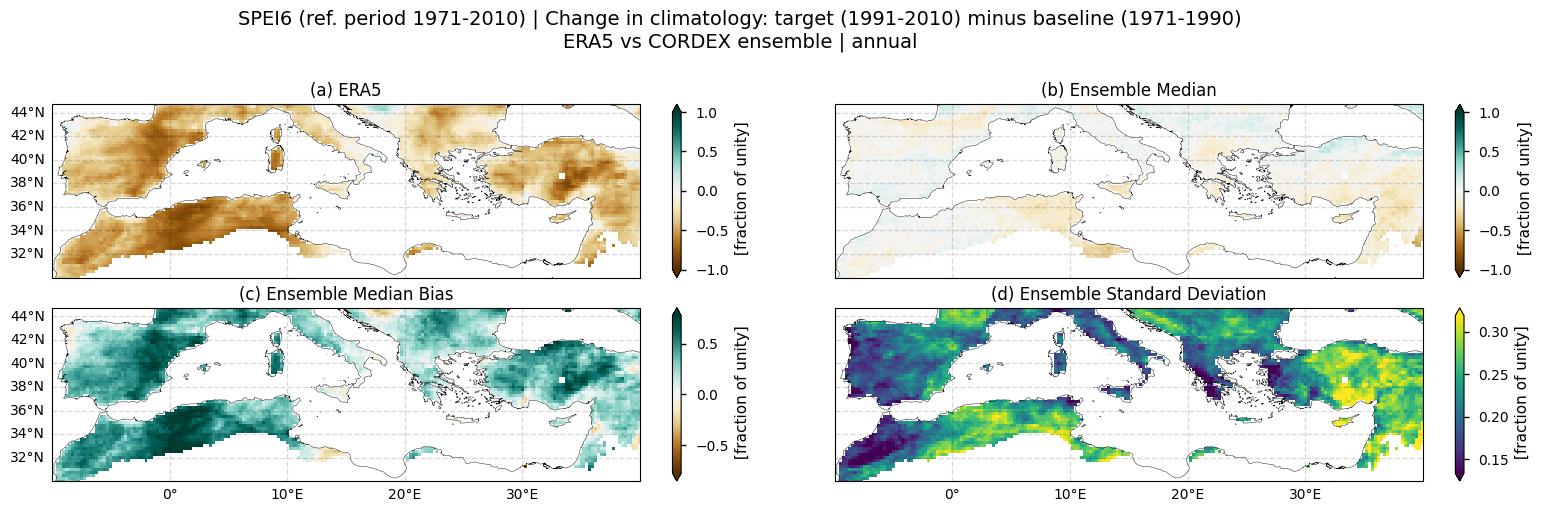
Fig 1. Spatial patterns of SPEI6 change over the Mediterranean region. Panels show (a) ERA5 reference, (b) CORDEX ensemble median (median of the selected subset of models at each grid cell), (c) ensemble median bias relative to ERA5, and (d) ensemble spread (standard deviation across the selected models). SPEI6 is standardised over the reference period 1971–2010. SPEI6 change is calculated at each grid point as the difference between the monthly climatologies of the target period (1991–2010) and the baseline period (1971–1990), and then averaged to obtain the ANNUAL mean.

NOTE:
The regridding artefacts visible in panel (d) result from the use of a conservative regridding method, which is commonly recommended when dealing with precipitation. They typically arise from large values in specific models and differences among the models’ native grids.

3.3. Plot ensemble maps - Seasonal aggregations#

Same as 3.2 section but for: DJF, MAM, JJA and SON

WINTER (DJF)

../../_images/f28dae91907430a4183132006b3e0488e262c26118ca22e911c0417f98d9f053.png

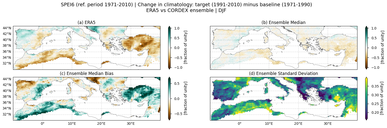
Fig 2. Spatial patterns of SPEI6 change over the Mediterranean region. Panels show (a) ERA5 reference, (b) CORDEX ensemble median (median of the selected subset of models at each grid cell), (c) ensemble median bias relative to ERA5, and (d) ensemble spread (standard deviation across the selected models). SPEI6 is standardised over the reference period 1971–2010. SPEI6 change is calculated at each grid point as the difference between the monthly climatologies of the target period (1991–2010) and the baseline period (1971–1990), and then averaged across the winter to obtain the DJF mean.

SPRING (MAM)

../../_images/597221777f38521193f40fa8f2eff134a5e1223c594b9562ee1ac3ceebeb25b2.png

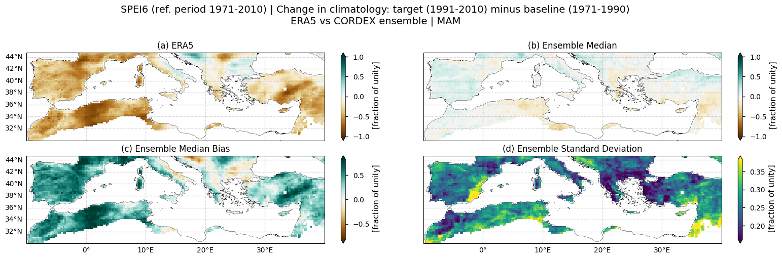
Fig 3. Spatial patterns of SPEI6 change over the Mediterranean region. Panels show (a) ERA5 reference, (b) CORDEX ensemble median (median of the selected subset of models at each grid cell), (c) ensemble median bias relative to ERA5, and (d) ensemble spread (standard deviation across the selected models). SPEI6 is standardised over the reference period 1971–2010. SPEI6 change is calculated at each grid point as the difference between the monthly climatologies of the target period (1991–2010) and the baseline period (1971–1990), and then averaged across the spring to obtain the MAM mean.

SUMMER (JJA)

../../_images/d7d16d12d1a2be3399748ed066fb77ac92409252173dbdad972450c8b342c7bf.png

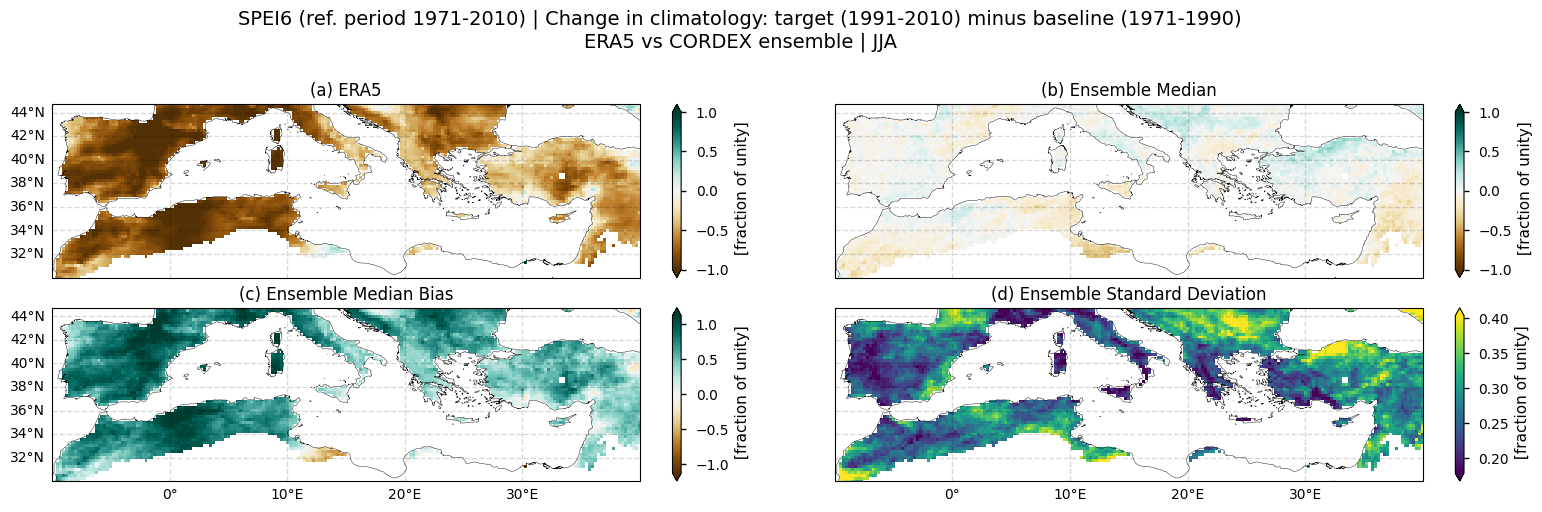
Fig 4. Spatial patterns of SPEI6 change over the Mediterranean region. Panels show (a) ERA5 reference, (b) CORDEX ensemble median (median of the selected subset of models at each grid cell), (c) ensemble median bias relative to ERA5, and (d) ensemble spread (standard deviation across the selected models). SPEI6 is standardised over the reference period 1971–2010. SPEI6 change is calculated at each grid point as the difference between the monthly climatologies of the target period (1991–2010) and the baseline period (1971–1990), and then averaged across the summer to obtain the JJA mean.

AUTUMN (SON)

../../_images/25a6b80cb899d3f1877bcf430bc70708d9a25f07ae3635096659e2c29f565ba2.png

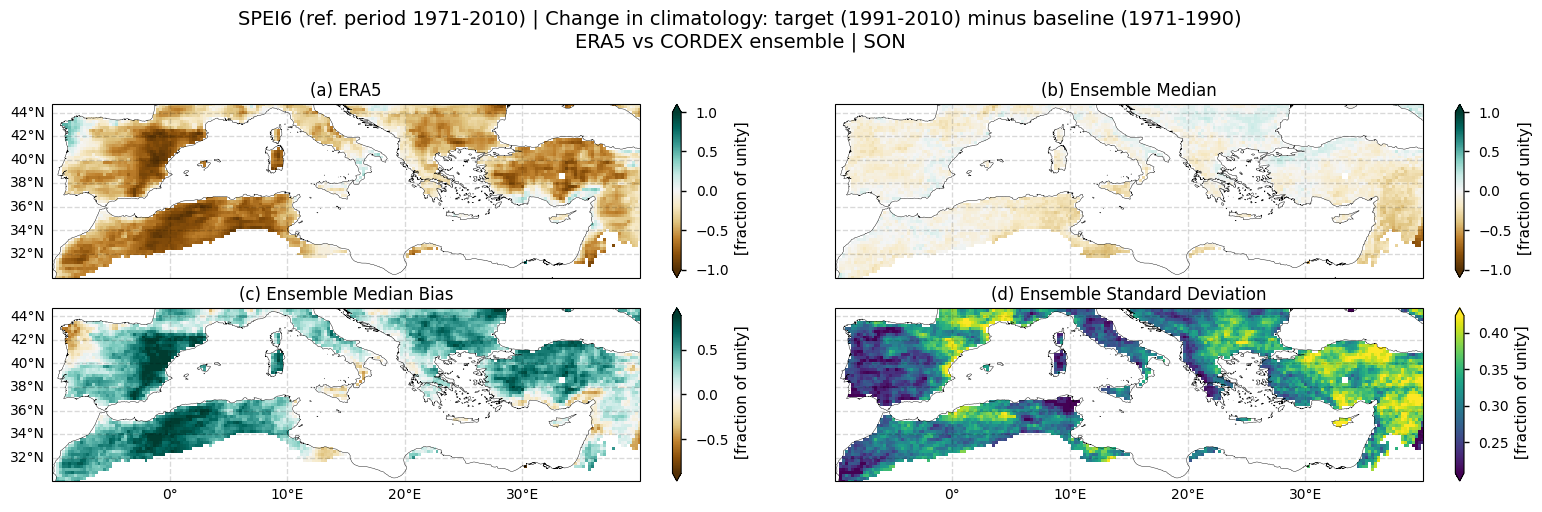
Fig 5. Spatial patterns of SPEI6 change over the Mediterranean region. Panels show (a) ERA5 reference, (b) CORDEX ensemble median (median of the selected subset of models at each grid cell), (c) ensemble median bias relative to ERA5, and (d) ensemble spread (standard deviation across the selected models). SPEI6 is standardised over the reference period 1971–2010. SPEI6 change is calculated at each grid point as the difference between the monthly climatologies of the target period (1991–2010) and the baseline period (1971–1990), and then averaged across the autumn to obtain the SON mean.

3.4. Plot model maps#

In this section, we invoke the plot_models() function to visualise the SPEI6 change of every model individually. Note that the model data used in this section maintains its original grid. Only the annual mean is shown here.

../../_images/6f11fe14ce33a9352d6662cce23e9a27c45d2e6e289ede860452c2bcae05966c.png

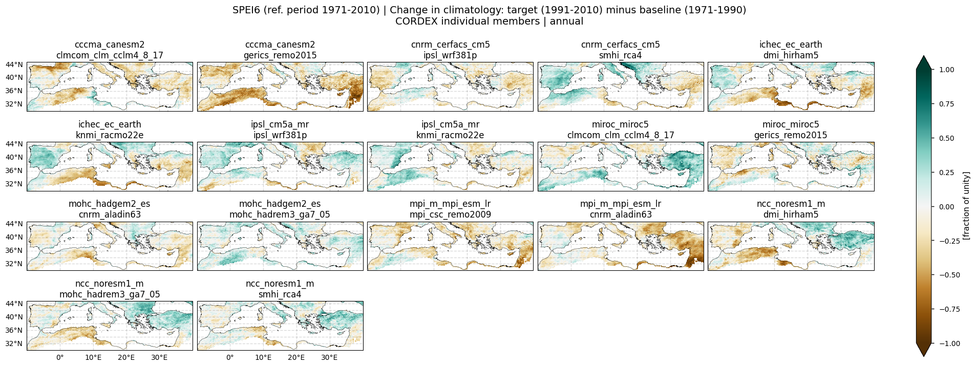
Fig 6. Spatial patterns of SPEI6 change for each individual CORDEX model over the Mediterranean region. SPEI6 is standardised over the reference period 1971–2010. For each model, SPEI6 change is calculated at each grid point as the difference between the monthly climatologies of the target period (1991–2010) and the baseline period (1971–1990), and then averaged to obtain the annual mean.

3.5. Plot bias maps#

In this section, we invoke the plot_models() function to visualise the bias of the SPEI6 change for every model individually. Note that the model data used in this section has previously been interpolated to the ERA5 grid. Regridding is performed for each essential climate variable before the index calculation to preserve standardisation. Only the annual mean is shown here.

../../_images/29c25cdfe0dc0ed72f72ae8fcc8f6d66893240b9762ac2c81b319b80a6346388.png

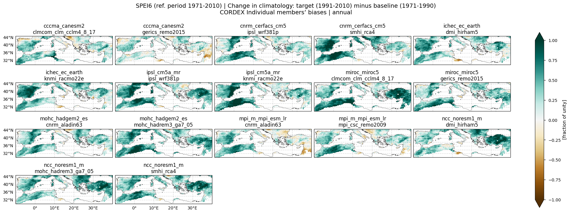
Fig 7. Bias of SPEI6 change for each individual CORDEX model relative to ERA5 over the Mediterranean region. SPEI6 is standardised over the reference period 1971–2010. For each model and ERA5, SPEI6 change is calculated at each grid point as the difference between the monthly climatologies of the target period (1991–2010) and the baseline period (1971–1990), and then averaged to obtain the annual mean.

3.6. Timeseries#

This section shows the timeseries of SPEI6 anomalies relative to the baseline climatology. We first use compute_change_4timeseries(), which calculates SPEI6 anomalies for each month of the timeseries (relative to the baseline monthly climatologies) and aggregates them according to the time_agg parameter. Spatially averaged values are then obtained. Light blue shading highlights the baseline period, while light orange shading marks the target period. The analysis compares the CORDEX ensemble median, ERA5, and individual models, displaying trends for both ERA5 and the ensemble median. Additionally, it shows the ensemble spread and the slope values of the trends for ERA5 and the CORDEX ensemble median. Only the annual aggregation is shown here.

Show code cell source

Hide code cell source

# Define colors
colors = {"CORDEX": "green", "ERA5": "black"}

# Cutout region
regionalise_kwargs = {
    "lon_slice": slice(area[1], area[3]),
    "lat_slice": slice(area[0], area[2]),
}

# Compute the change/anomaly for ERA5
ds_era5_change = compute_change_4timeseries(ds_era5, baseline_slice, time_agg)

# Regionalise and compute spatially weighted mean
era5_mean = diagnostics.spatial_weighted_mean(
    utils.regionalise(ds_era5_change, **regionalise_kwargs)
)
era5_mean["year"]=pd.to_datetime(era5_mean["year"].values, format='%Y')


# Compute change/anomaly for each model and spatially aggregate
cordex_means = []
for model, ds in model_datasets.items():
    ds_model_change = compute_change_4timeseries(ds, baseline_slice, time_agg)
    ds_model_change["year"]=pd.to_datetime(ds_model_change["year"].values, format='%Y')
    ds_model_regional = utils.regionalise(ds_model_change, **regionalise_kwargs)
    cordex_mean = diagnostics.spatial_weighted_mean(ds_model_regional)
    cordex_means.append(cordex_mean)

# Ensemble statistics
cordex_stack = xr.concat(cordex_means, dim="model")
cordex_var = cordex_stack.median("model", keep_attrs=True)
cordex_std = cordex_stack.std("model", keep_attrs=True)

# Initialize plot
plt.figure(figsize=(10, 5))

ax = plt.gca()

# Shade baseline period (light blue)
ax.axvspan(
    pd.to_datetime(str(baseline_slice.start)),
    pd.to_datetime(str(baseline_slice.stop)),
    color="lightblue",
    alpha=0.3,
)

# Shade target period (light orange)
ax.axvspan(
    pd.to_datetime(str(target_slice.start)),
    pd.to_datetime(str(target_slice.stop)),
    color="peachpuff",
    alpha=0.3,
)

# --- Create custom legend entries with full opacity ---
baseline_patch = mpatches.Patch(color="lightblue", alpha=0.8, label="Baseline period")
target_patch = mpatches.Patch(color="peachpuff", alpha=0.8, label="Target period")

# Plot individual model time series
for model_data in cordex_means:
    model_values = model_data.values.flatten() if model_data.ndim > 1 else model_data.values
    plt.plot(model_data['year'], model_values, linestyle='-', color="grey", alpha=0.4)

# Add legend entry for individual models
plt.plot([], [], linestyle='-', color='grey', alpha=0.3, label='Individual Models')

# Plot ERA5
era5_mean.plot(label="ERA5", color=colors["ERA5"])

# Plot CORDEX median
cordex_var.plot(label="CORDEX Median", color=colors["CORDEX"])

# Fill ±1 std (spread)
plt.fill_between(
    cordex_var['year'],
    cordex_var.values - cordex_std.values,
    cordex_var.values + cordex_std.values,
    color = colors["CORDEX"],
    alpha = 0.4,
    label = "CORDEX Spread"
)

# Compute trends
slope_era5, p_value_era5 = plot_trend(
    era5_mean['year'][~np.isnan(era5_mean.values)],
    era5_mean.values[~np.isnan(era5_mean.values)],
    "ERA5 Trend",
    colors["ERA5"]
)

slope_cordex, p_value_cordex = plot_trend(
    cordex_var['year'][~np.isnan(cordex_var.values)],
    cordex_var.values[~np.isnan(cordex_var.values)],
    "CORDEX Median Trend",
    colors["CORDEX"]
)

trend_info = [
    ("ERA5", slope_era5, p_value_era5),
    ("CORDEX Median", slope_cordex, p_value_cordex)
]

# Labels and grid
plt.xlabel('Year')
plt.ylabel("Fraction of unity")
title = (f"SPEI{window} (ref. period {reference_slice.start}-{reference_slice.stop}) | Change rel. to {baseline_slice.start}-{baseline_slice.stop}\n"
        f"Target period: ({target_slice.start}-{target_slice.stop}) | {time_agg}")

plt.title(title)

    
plt.legend()
plt.grid(True)

# Format x-axis as years
ax = plt.gca()
ax.xaxis.set_major_formatter(mdates.DateFormatter('%Y'))
plt.gcf().autofmt_xdate()

# Annotate trends
plt.gcf().text(
    0.5, -0.015,
    '\n'.join([
        f"{name} Trend: {trend:.4f} (fraction of unity/decade), p-value: {p:.3e}"
        for name, trend, p in trend_info
    ]),
    fontsize=12,
    ha='center',
    va='center',
    bbox=dict(boxstyle="square,pad=0.5", edgecolor="black", facecolor="lightgray")
)

plt.ylim((-1.7, 1.7))
plt.show()

../../_images/6ef0f20319d8771f66144f69982812e3d72bae3b9e1973200aeb21f39305575a.png

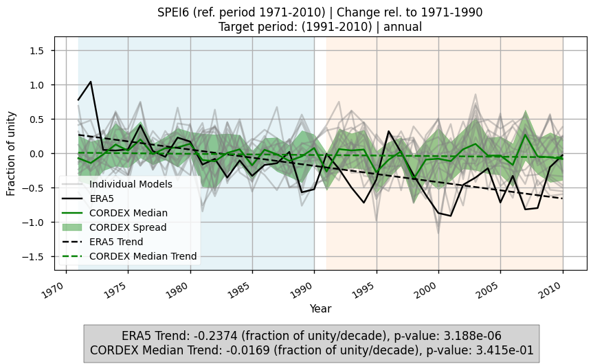
Fig 8. Timeseries of SPEI6 anomalies over the Mediterranean region. Monthly anomalies are calculated relative to the monthly baseline climatologies, aggregated according to the specified timescale, and then spatially averaged over the region. Light blue shading indicates the baseline period, and light orange shading indicates the target period. The figure compares ERA5, the CORDEX ensemble median, and individual models, showing trends for ERA5 and the ensemble median, as well as the ensemble spread and slope values of the trends.

3.7. Results summary#

ERA5 indicates a general intensification of drought conditions over the Mediterranean region when comparing the baseline (1971–1990) and target (1991–2010) periods.
The CORDEX ensemble median (obtained from the subset of models considered within this notebook) of the SPEI6 change is generally close to zero (Fig. 1). However, the inter-model spread is high, and is particularly pronounced over the Iberian Peninsula, southern France, North Africa, the Balkans region, and the easternmost Mediterranean areas (including Turkey, Lebanon, and Syria). In fact, the spatial pattern of the SPEI6 change is pretty different depending on the considered model (Fig. 6 and 7).
Seasonal analysis (Figs. 2–5) indicates that, in ERA5, drought intensification is strongest in summer. Spring and autumn also show notable decreases in SPEI6, although localised increases partly offset the spatial mean, especially in spring. In winter, the sign of the SPEI6 change is region-dependent, with large decreases over the eastern Iberian Peninsula, the eastern Mediterranean, and North Africa, and increases over the western Iberian Peninsula, as well as parts of Italy and the Balkans. Considering the CORDEX ensemble median, SPEI6 changes remain close to zero for most seasons and regions, with no clear spatial patterns overall, or at least none consistent with those observed in ERA5.
The timeseries of spatial means over the Mediterranean confirms an increase in drought conditions during the considered historical period in ERA5, with a trend of –0.24 (Fig. 8). For the ensemble median of CORDEX, the timeseries shows a trend close to zero, which is also not statistically significant. The timeseries plot also shows a high inter-model spread. Timeseries for seasonal aggregations are not shown here, but have been computed offline and exhibit behaviour similar to the annual case.
The results obtained in this notebook differ from those reported in the quality assessment named CMIP6 biases in the SPEI6 drought index over the Mediterranean region, where CMIP6 ensemble median captured the sign of the SPEI6 change for a similar historical period, although with an underestimation compared to ERA5.
The limited change in SPEI6 simulated by some CORDEX models, compared to ERA5 and the previous CMIP6-based counterpart assessment, may partly reflect methodological and structural factors. In particular, the shorter analysis periods used here (20-year blocks instead of 30) may reduce the robustness of the signal. In addition, many CORDEX RCMs do not include time-evolving aerosols, which can lead to an underestimation of temperature trends in some regions and consequently affect drought-related indices such as SPEI6 [9].

3.8. Implications for the users#

The pronounced inter-model spread over North Africa, Turkey, and the eastern Mediterranean implies that users in these regions may face higher future uncertainty. This highlights the need to stress-test adaptation strategies against a wide range of plausible futures rather than relying on a single scenario.
Although the ensemble median does not capture the SPEI6 change signal for the historical period, this does not necessarily imply that the models are not suitable for investigating future changes, as the spatial pattern of change depends on the individual model considered and model biases are not necessarily stationary, but may evolve under changing climate conditions [10].
The approach used in this notebook illustrates how a subset of GCM–RCM combinations can be selected while maintaining representation of all driving GCMs. This can be useful in situations where computational or practical constraints limit the use of the full ensemble. However, the results also reinforce that broader ensembles provide a more robust basis for assessing uncertainty.
Finally, users should be aware that results may vary depending on the choice of historical periods and model configurations. In this context, complementary tools such as the C3S Atlas, which includes a larger ensemble and alternative period definitions, can provide additional context for interpreting these findings. In addition, this notebook helps users understand the basis of the SPEI index and its methodological assumptions, supporting its application in operational water management and drought preparedness.

ℹ️ If you want to know more#

Key resources#

Some key resources and further reading were linked throughout this assessment.

The CDS catalogue entries for the data used were:

CORDEX regional climate model data on single levels (daily - Maximum 2m temperature in the last 24 hours, Minimum 2m temperature in the last 24 hours, 2m air temperature and Mean precipitation flux): https://cds.climate.copernicus.eu/datasets/projections-cordex-domains-single-levels?tab=overview
ERA5 hourly data on single levels from 1940 to present (2m temperature and total precipitation): https://cds.climate.copernicus.eu/datasets/reanalysis-era5-pressure-levels-monthly-means?tab=overview

Code libraries used:

C3S EQC custom functions, c3s_eqc_automatic_quality_control, prepared by B-Open

References#

[1] Vicente-Serrano, S. M., Beguerı́a, S., and López-Moreno, J. I., 2010. A multiscalar drought index sensitive to global warming: The standardized precipitation evapotranspiration index, Journal of Climate, 23, 1696–1718. https://doi.org/10.1175/2009JCLI2909.1

[2] Wilhite, D. A., 2000. Droughts as a natural hazard: concepts and definitions. In: DROUGHT, A Global Assessment, vol. I and II, Routledge Hazards and Disasters Series, Routledge.

[3] Vicente-Serrano, S. M., Beguerı́a, S., Lorenzo-Lacruz, J., Camarero, J. J., López-Moreno, J. I., Azorin-Molina, C., Revuelto, J., Morán-Tejeda, E., and Sanchez-Lorenzo, A., 2012. Performance of drought indices for ecological, agricultural, and hydrological applications, Earth Interactions, 16, https://doi.org/10.1175/2012EI000434.1

[4] Kalisoras, A., Georgoulias, A. K., Akritidis, D., and Zanis, P., 2025. Future Projections in Agricultural Drought Characteristics for Greece Under Different Climate Change Scenarios. Environmental and Earth Sciences Proceedings, 35(1), 29. https://doi.org/10.3390/eesp2025035029

[5] Spinoni, J., Barbosa, P., Bucchignani, E., Cassano, J., Cavazos, T., Cescatti, A., Christensen, J. H., Christensen, O. B., Coppola, E., Evans, J. P., Forzieri, G., Geyer, B., Giorgi, F., Jacob, D., Katzfey, J., Koenigk, T., Laprise, R., Lennard, C. J., Kurnaz, M. L., … Dosio, A., 2021. Global exposure of population and land-use to meteorological droughts under different warming levels and SSPs: A CORDEX-based study. International Journal of Climatology, 41(15), 6825–6853. https://doi.org/10.1002/joc.7302

[6] Iturbide, M., Gutiérrez, J. M., Alves, L. M., Bedia, J., Cerezo-Mota, R., Cimadevilla, E., Cofiño, A. S., Di Luca, A., Faria, S. H., Gorodetskaya, I. V., Hauser, M., Herrera, S., Hennessy, K., Hewitt, H. T., Jones, R. G., Krakovska, S., Manzanas, R., Martínez-Castro, D., Narisma, G. T., Nurhati, I. S., Pinto, I., Seneviratne, S. I., van den Hurk, B., and Vera, C. S., 2020. An update of IPCC climate reference regions for subcontinental analysis of climate model data: definition and aggregated datasets, Earth Syst. Sci. Data, 12, 2959–2970, https://doi.org/10.5194/essd-12-2959-2020

[7] Hargreaves, G. H., and Samani, Z. A., 1985. Reference crop evapotranspiration from temperature, Applied engineering in agriculture, pp. 96–99. https://doi.org/10.13031/2013.26773

[8] Beguerı́a, S., Vicente-Serrano, S. M., Reig, F., and Latorre, B., 2014. Standardized precipitation evapotranspiration index (spei) revisited: Parameter fitting, evapotranspiration models, tools, datasets and drought monitoring, International Journal of Climatology, 34, 3001–3023. https://doi.org/10.1002/joc.3887

[9] Schumacher, D.L., Singh, J., Hauser, M., et al., 2024. Exacerbated summer European warming not captured by climate models neglecting long-term aerosol changes. Commun Earth Environ 5, 182. https://doi.org/10.1038/s43247-024-01332-8

[10] Schmith, T., Thejll, P., Berg, P., Boberg, F., Christensen, O. B., Christiansen, B., Christensen, J. H., Madsen, M. S., and Steger, C., 2021. Identifying robust bias adjustment methods for European extreme precipitation in a multi-model pseudo-reality setting, Hydrol. Earth Syst. Sci., 25, 273–290, https://doi.org/10.5194/hess-25-273-2021

CORDEX biases in the SPEI6 drought index over the Mediterranean region

Contents

5.2.7. CORDEX biases in the SPEI6 drought index over the Mediterranean region#

🌍 Use case: Calculating drought indices from climate projections data to inform water management#

❓ Quality assessment question#

📢 Quality assessment statement#

📋 Methodology#

📈 Analysis and results#

1. Parameters, requests and functions definition#

1.1. Import packages#

1.2. Define Parameters#

1.3. Define models#

1.4. Define ERA5 request#

1.5. Define model requests#

1.6. Functions to cache#

2. Downloading and processing#

2.1. Download and transform ERA5#

2.2. Download and transform models#

2.3. Apply land-sea mask and change some attributes#

3. Plot and describe results#

3.1. Define plotting functions#

3.2. Plot ensemble maps#

3.3. Plot ensemble maps - Seasonal aggregations#

3.4. Plot model maps#

3.5. Plot bias maps#

3.6. Timeseries#

3.7. Results summary#

3.8. Implications for the users#

ℹ️ If you want to know more#

Key resources#

References#