

1.4.6. Satellite Land Cover trend assessment for Spatial Planning and Land Management#
Production date: 01-07-2024
Produced by: Inês Girão (+ATLANTIC)
🌍 Use case: Using land cover products to quantify urbanisation trends#
❓ Quality assessment question#
Is the dataset accurate and consistent for the analysis of urbanisation trends in the Iberian Peninsula?
Land Cover data is an invaluable resource for a wide range of fields, from climate change research to urban planning. Land Cover products that provide historical timelines enable scientists, policymakers, and planners to understand and analyse the transformation of land cover over recent decades (Vargo et al, 2013; Chang et al., 2018).
This notebook will access the Land cover classification gridded maps from 1992 to present derived from satellite observations (henceforth, LC) data from the Climate Data Store (CDS) of the Copernicus Climate Change Service (C3S), and analyse the spatial patterns of the LC over a given Area of Interest (AoI) and time.
📢 Quality assessment statement#
These are the key outcomes of this assessment
The dataset maintains strong temporal continuity, with annual updates ensuring a smooth and reliable representation of land cover changes over time. While breakpoints were identified, they generally did not indicate major disruptions, reinforcing the dataset’s stability for long-term trend analysis.
The presence of breakpoints does not necessarily indicate abrupt landscape shifts but rather highlights the sensitivity of detection methods to gradual changes. This suggests that while breakpoints can help refine analysis, their impact on overall trends remains limited, emphasising the dataset’s resilience to minor variations.
For the specific land cover type analysed, the dataset exhibits a consistent ability to capture underlying trends. The similarity in results across segmented and total trends suggests that the data structure is well-calibrated, minimising distortions that could arise from classification inconsistencies or methodological biases.

📋 Methodology#
This Use Case comprises the following steps:
1. Define the AoI, search and download LC data
2. Inspect and view data for the defined AoI (Iberian Peninsula)
📈 Analysis and results#
1. Define the AoI, search and download LC data#
Before we begin we must prepare our environment. This includes installing the Application Programming Interface (API) of the CDS, and importing the various python libraries that we will need.
Install CDS API#
To install the CDS API, run the following command. We use an exclamation mark to pass the command to the shell (not to the Python interpreter). If you already have the CDS API installed, you can skip or comment this step.
Import all the libraries/packages#
We will be working with data in NetCDF format. To best handle this type of data we will use libraries for working with multidimensional arrays, in particular Xarray. We will also need libraries for plotting and viewing data.
Data Overview#
To search for data, visit the CDS website: https://cds.climate.copernicus.eu Here you can search for ‘Satellite observations’ using the search bar. The data we need for this tutorial is the Land cover classification gridded maps from 1992 to present derived from satellite observations. This catalogue entry provides global Land Cover Classification (LCC) maps with a very high spatial resolution, with a L4 processing level, on an annual basis with a one-year delay, following the Global Climate Observing System (GCOS) convention requirements. LULC maps correspond to a global classification scheme, encompassing 22 classes.
The dataset consists of 2 versions (v2.0.7 produced by the European Space Agency (ESA) Climate Change Initiative (CCI) and v2.1.1 produced by Copernicus Climate Change Service (C3S)).
Data specifications for this use case:
Years: 1992 to 2022
Version: v2.0.7 before 1992 and v2.1.1 after 2016
Format: Zip files
At the end of the download form, select “Show API request”. This will reveal a block of code, which you can simply copy and paste into a cell of your Jupyter Notebook. Having copied the API request, running it will retrieve and download the data you requested into your local directory. However, before you run it, the terms and conditions of this particular dataset need to have been accepted directly at the CDS website. The option to view and accept these conditions is given at the end of the download form, just above the “Show API request” option. In addition, it is also useful to define the time period and AoI parameters and edit the request accordingly, as exemplified in the cells below.
<xarray.Dataset> Size: 7GB
Dimensions:              (year: 31, latitude: 3600, longitude: 5040, bounds: 2)
Coordinates:
  * year                 (year) int64 248B 1992 1993 1994 ... 2020 2021 2022
  * latitude             (latitude) float64 29kB 45.0 45.0 44.99 ... 35.0 35.0
  * longitude            (longitude) float64 40kB -9.999 -9.996 ... 3.996 3.999
    lat_bounds           (latitude, bounds, longitude) float64 290MB dask.array<chunksize=(1200, 1, 1680), meta=np.ndarray>
    lon_bounds           (longitude, bounds) float64 81kB dask.array<chunksize=(5040, 2), meta=np.ndarray>
    time_bounds          (year, bounds, longitude) datetime64[ns] 2MB dask.array<chunksize=(1, 2, 5040), meta=np.ndarray>
Dimensions without coordinates: bounds
Data variables:
    lccs_class           (year, latitude, longitude) uint8 562MB dask.array<chunksize=(1, 1800, 2520), meta=np.ndarray>
    processed_flag       (year, latitude, longitude) float32 2GB dask.array<chunksize=(1, 1800, 2520), meta=np.ndarray>
    current_pixel_state  (year, latitude, longitude) float32 2GB dask.array<chunksize=(1, 1800, 2520), meta=np.ndarray>
    observation_count    (year, latitude, longitude) uint16 1GB dask.array<chunksize=(1, 1800, 2520), meta=np.ndarray>
    change_count         (year, latitude, longitude) uint8 562MB dask.array<chunksize=(1, 1800, 2520), meta=np.ndarray>
    crs                  (year, longitude) int32 625kB dask.array<chunksize=(1, 5040), meta=np.ndarray>
Attributes: (12/38)
    id:                         ESACCI-LC-L4-LCCS-Map-300m-P1Y-1992-v2.0.7cds
    title:                      Land Cover Map of ESA CCI brokered by CDS
    summary:                    This dataset characterizes the land cover of ...
    type:                       ESACCI-LC-L4-LCCS-Map-300m-P1Y
    project:                    Climate Change Initiative - European Space Ag...
    references:                 http://www.esa-landcover-cci.org/
    ...                         ...
    geospatial_lon_max:         180
    spatial_resolution:         300m
    geospatial_lat_units:       degrees_north
    geospatial_lat_resolution:  0.002778
    geospatial_lon_units:       degrees_east
geospatial_lon_resolution: 0.0027782. Inspect and view data for the defined AoI (Iberian Peninsula)#
Compute urban area for each NUTS 2 region#
To identify changes in LC patterns, in this user question, NUTS 2 will be used, providing the information regarding the main regions of the Iberian Peninsula.
The NUTS are a hierarchical system divided into 3 levels. NUTS 1 correspond to major socio-economic regions, NUTS 2 correspond to basic regions for the application of regional policies, and NUTS 3 correspond to small regions for specific diagnoses. Additionally a NUTS 0 level, usually co-incident with national boundaries is also available. The NUTS legislation is periodically amended; therefore multiple years are available for download.
The step below masks the Land Cover data according to the NUTS 2 boundaries and calculate the area of each pixel (weighted by the cosine of Latitude). For each NUTS 2, we proceed with the analysis and visual inspection of Land Cover areas per class and corresponding percentages during the elected period.
Mask regions#
First, we need to establish the geometry of the NUTS region (level 2) in order to make the corresponding statistics.
Compute cell area#
Then, we can calculate the area of each pixel taking into consideration the curvature of the earth (i.e., weighted by the cosine of Latitude).
Select Urban Classes and Prepare Dataset#
Compute urban area per region and year#
Map urban percentage coverage over-time by NUTS regions in the AoI#
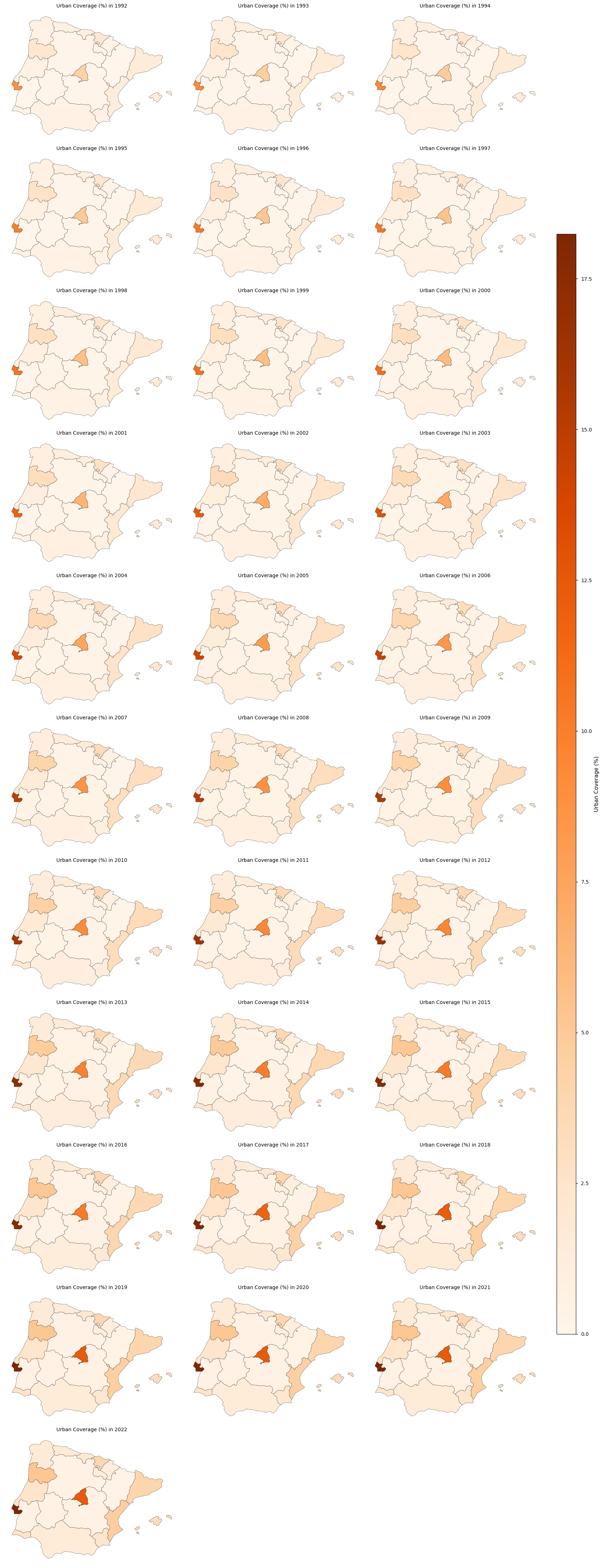
Map Analysis#
Over the 28-year period, all regions maintain a consistent pattern of growth.
Regions such as Comunidad Madrid and Área Metropolitana de Lisboa consistently exhibit the highest levels of urban percentage coverage.
No negative fluctuations were observed
The biggest changes are observed between 2016-2017.
Potential Drivers and Methodological Considerations in Urbanisation Trends in the Iberian Peninsula (1992–2022)#
Urbanisation in the Iberian Peninsula over the last three decades has been influenced by a combination of economic shifts, demographic changes, and policy decisions. Before analysing trends, it is essential to account for abrupt shifts that may distort trend estimates. These shifts, often referred to as breakpoints, can result from:
Economic Drivers
Economic Growth and Real Estate Booms: The rapid expansion of urban areas in Madrid, Barcelona, and Lisbon was driven by economic growth and increased investment in housing and infrastructure, particularly during the 1996–2007 real estate boom (González & Leal, 2018). The expansion of suburban areas led to the rise of peri-urban developments in regions like Valencia and Porto (Silva et al., 2017).
Economic Crisis (2008–2013): The 2008 financial crisis led to a slowdown in urban expansion, particularly in southern Spain, where unfinished developments and ghost towns became a common sight (Martínez & García, 2015). However, in some areas, reduced construction pressure allowed for the recovery of natural land cover (Palmero-Iniesta et al., 2021).
Demographic and Social Changes
Rural Depopulation: Migration from rural areas to urban centers, particularly among younger populations, has led to declining populations in Extremadura, Castilla y León, and Alentejo, accelerating the abandonment of agricultural lands and increasing the expansion of urban areas (Sánchez et al., 2019).
Tourism and Second-Home Development: The rise of tourism-driven urbanisation has significantly reshaped coastal regions like the Costa del Sol, Algarve, and the Balearic Islands, where seasonal housing developments have expanded rapidly (Rullan, 2014).
Aging Population: Aging populations in rural regions have led to increased urban migration, further depopulating countryside areas and concentrating populations in cities like Seville, Valencia, and Bilbao (Gutiérrez et al., 2016).
Infrastructure and Policy Influences
EU-Funded Infrastructure Projects: Investments in transport networks, such as the expansion of high-speed rail (AVE) in Spain and Alfa Pendular in Portugal, have facilitated suburbanisation and commuting from secondary urban centers (López et al., 2017).
Urban Planning Policies: The implementation of urban growth controls and greenbelt policies in cities like Barcelona and Porto has influenced spatial expansion patterns, sometimes leading to increased land prices and informal settlements (Silva & Fernandes, 2019).
Smart Cities and Sustainability Initiatives: Recent efforts to create more sustainable urban environments, such as Madrid’s Madrid Central low-emission zone, have shaped urbanisation patterns, promoting compact city models (Delgado & Romero, 2021).
Methodology
Certain shifts in urban land cover may be related to data collection and processing rather than actual urban expansion. For instance, transitions between different satellite sensors can introduce artificial breaks in the time series (Chelali et al., 2019).
The LC dataset is generated from a multi-sensor surface reflectance time series derived from several satellite missions. As sensor technology evolved, different instruments were used to produce consistent global composites.
Surface Reflectance (SR) Input |
Reference Period |
Satellite Sensor / Mission |
Main Characteristics |
|---|---|---|---|
AVHRR SR composites |
1992–1999 |
AVHRR-2 (NOAA-11, NOAA-14) |
~1 km spatial resolution, visible and near-infrared observations |
SPOT-VGT SR composites |
1999–2013 |
SPOT-4 / SPOT-5 VEGETATION |
1 km spatial resolution, 4 spectral bands (blue, red, NIR, SWIR) |
MERIS SR composites |
2003–2012 |
Envisat MERIS |
~300 m spatial resolution, 15 spectral bands in visible and near-infrared |
PROBA-V SR composites |
2013–2019 |
PROBA-V |
~300 m spatial resolution, 4 spectral bands (blue, red, NIR, SWIR) |
Sentinel-3 SR composites |
2020 |
Sentinel-3 OLCI |
~300 m spatial resolution, multispectral observations |
Sentinel-3 SR composites |
2021–2022 |
Sentinel-3 OLCI + SLSTR |
Optical and thermal observations supporting land-cover mapping |
Due to the limited spatial resolution of early sensors (AVHRR and SPOT-VGT), reliable detection of annual urban change was challenging prior to 2003. During this period, the representation of urban areas is guided by reference urban footprints derived from the Global Human Settlement Layer (GHSL) datasets for 1990 and 2000. These datasets provide baseline constraints for the urban class within the 1992–1999 and 2000–2003 epochs, helping to stabilise the detection of urban areas while still allowing minor variations arising from classification adjustments and mixed-pixel effects. From 2003 onwards, urban areas are derived from higher-resolution observations. To ensure temporal consistency, urban areas are only allowed to expand over time, and the resulting footprint is constrained between a minimum extent defined by GHSL 2000 and a maximum extent defined by GHSL 2014 (C3S - LC Algorithm Theoretical Basis Document, 2024).
In addition, the Global Urban Footprint (GUF) dataset is combined with GHSL 2014 to reduce potential omissions of built-up areas (C3S - LC Algorithm Theoretical Basis Document, 2024).
In addition to optical surface reflectance observations, auxiliary datasets are used to improve land-cover mapping. In particular, Envisat ASAR Wide Swath Mode (WSM) radar observations (2005–2012) are incorporated as ancillary information (C3S - LC Target Requirements and Gap Analysis Document, 2024).
While the dataset relies on multiple satellite sensors, it is not generated through simple sensor-to-sensor transitions. Instead, the global land-cover time series is built around a baseline land-cover map derived from MERIS observations (2003–2012). Earlier periods (1992–2003) are reconstructed through back-dating using AVHRR and SPOT-VGT data, while later years are produced through incremental updates using SPOT-VGT, PROBA-V, and Sentinel-3 observations. During several periods, multiple sensors are used simultaneously, with different roles (e.g., temporal consistency versus spatial refinement). As a result, potential discontinuities in the time series are more likely to arise from changes in processing strategy, data fusion, and constraints, rather than from simple sensor replacements.
Global LC database |
Reference period |
Satellite data source |
|---|---|---|
Baseline 10-year global LC map |
2003–2012 |
• MERIS FR/RR global SR composites between 2003 and 2012 |
Global annual LC maps |
1992–1999 |
• Baseline 10-year global LC map |
1999–2013 |
• Baseline 10-year global LC map |
|
2014–2019 |
• PROBA-V global SR composites at 1 km for years 2014 to 2019 for updating the baseline |
|
2020–2022 |
• S3 global SR composites at 1 km for years 2020 to 2022 for updating the baseline |
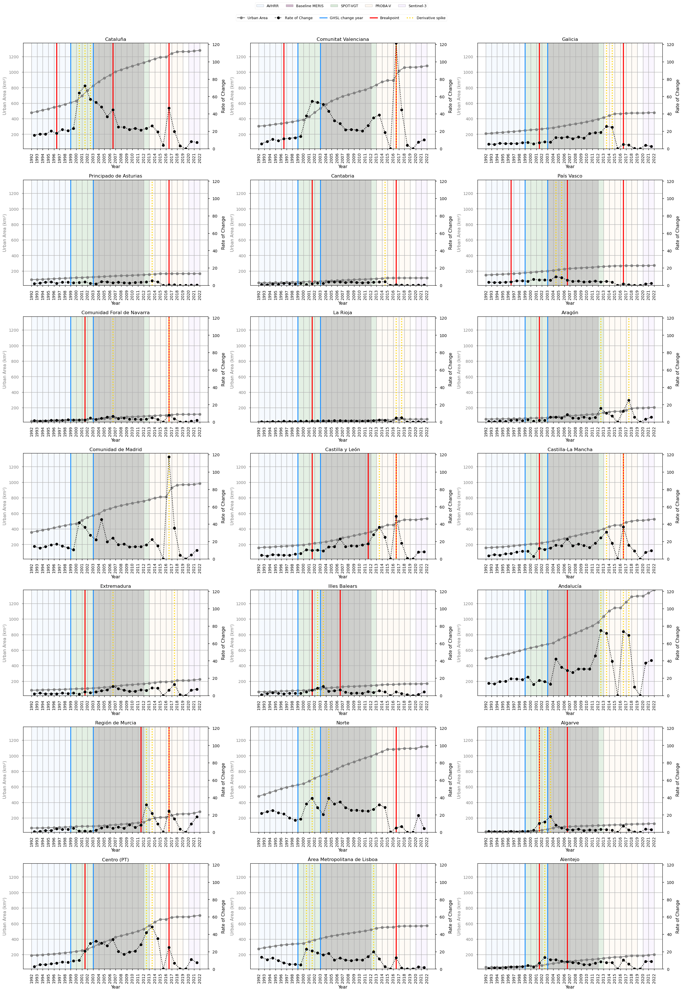
3. Breakpoint Detection#
A first step in assessing temporal behaviour is to analyse the rate of change of the urban-area time series. This provides an intuitive view of how the pace of urban expansion evolves over time and helps highlight periods where the trajectory deviates from its typical pattern.
However, while such exploratory diagnostics identify points of interest, they do not by themselves confirm whether the observed changes are structurally meaningful. Year-to-year variations may reflect noise, smoothing effects, or gradual adjustments in the underlying product. To formally assess structural changes, a statistical breakpoint detection method is applied.
The analysis therefore combines rate-of-change diagnostics with statistical segmentation, with particular attention to the monotonic nature of the data and the need to avoid over-interpreting gradual trends as discrete breakpoints.
Rate of Change Calculation
The first derivative of the urban-area time series is computed to quantify the year-to-year change in urban extent.
This highlights periods where the pace of urban expansion deviates from its typical behaviour, providing an initial indication of potential anomalies or shifts in the series.
Statistical Thresholding of Derivative Spikes
To identify unusually strong deviations, a dynamic threshold is defined as:
Threshold = mean(|rate of change|) + 1.5 × standard deviation
Years where the absolute rate of change exceeds this threshold are flagged as derivative spikes.
These spikes represent periods where the magnitude of change is unusually large relative to the typical variability of the series.
This step serves as a diagnostic indicator of anomalous growth behaviour, but does not in itself define structural breakpoints.
Breakpoint Detection Using the PELT Algorithm
The Pruned Exact Linear Time (PELT) algorithm is used to detect changes in the statistical behaviour of the growth rate, rather than in the cumulative urban-area series itself.
This is important because the urban-area time series is monotonic and non-decreasing, meaning that applying segmentation directly to the cumulative values can lead to artificial breakpoints driven by gradual growth.
The algorithm is therefore applied to the first derivative (growth rate), allowing detection of:
transitions between periods with different rates of urban expansion, rather than absolute levels.
The implementation uses:
the L2 cost function (
model="l2") to minimise variance within segments,a fixed penalty parameter (
pen = 2.5) applied to a standardised growth-rate series,and a minimum segment length (
min_size = 3) to avoid short, unstable segments.
Prior to segmentation, the growth-rate series may be standardised to ensure comparability across regions with different magnitudes of urban change.
Breakpoint Selection
Breakpoints are identified directly from the segmentation of the growth-rate series.
Unlike earlier approaches, no explicit filtering based on derivative spikes is applied, as this was found to introduce additional assumptions and potentially remove meaningful structural changes.
Instead, derivative spikes and breakpoints are analysed in parallel, allowing independent but complementary perspectives on the temporal behaviour of the series.
Methodological Considerations
The urban-area time series is strictly monotonic and cumulative by construction, reflecting constraints in the land-cover product that prevent decreases in urban extent.
As a result:
segmentation applied to the raw series tends to produce regularly spaced breakpoints, even in the absence of true structural changes.
applying breakpoint detection to the growth rate mitigates this issue by focusing on changes in dynamics rather than accumulated values.
Even when applied to growth rates, breakpoint detection should be interpreted cautiously:
some detected changes may reflect gradual adjustments in processing or classification, rather than abrupt real-world events.
others may correspond to genuine shifts in the pace of urban expansion.
For this reason, breakpoint detection is treated as a diagnostic tool, not as definitive evidence of discrete events.
Interpreting Breakpoint Timing
Breakpoint positions should be interpreted as approximate indicators of when a change in growth dynamics begins, rather than exact points of maximum change.
Because segmentation identifies changes in statistical behaviour, the detected breakpoint may:
precede the most visible increase in growth rate, or
occur within a broader transition period.
As a result, breakpoint timing should be considered indicative rather than exact, and interpreted in conjunction with derivative-based diagnostics.
To assess whether detected discontinuities in the urban-area time series may be influenced by methodological factors, a targeted alignment analysis is performed. The aim is to evaluate whether growth-rate breakpoints and derivative spikes occur shortly after known processing-chain changes.
For each detected event, the time difference relative to each processing-change year is computed. An event is considered potentially related to a processing change only if it occurs within the two years following that transition. This forward-looking window reflects the temporal characteristics of the dataset, where land-cover changes are only confirmed if they persist over two consecutive years.
In addition to temporal alignment, the analysis also considers the spatial consistency of detected signals, quantified as the number of regions affected within a given interval. Methodological effects are expected to influence the dataset in a systematic way, and therefore to appear consistently across multiple regions. In contrast, signals affecting only a small number of regions are more likely to reflect local dynamics or region-specific variations rather than processing-related artefacts.
The results are summarised in four complementary tables, distinguishing between:
Event type: breakpoints vs derivative spikes
Analytical scope: aligned vs full set of identified breakpoints and derivative spikes
The first two tables report only events that occur within two years after a processing transition, while the two additional tables report all detected events.
### Breakpoint alignment table ###
| Interval | Aligned signal intervals | Number of regions | Region names | Nearest processing changes |
|---|---|---|---|---|
| 2000-2002 | 2001-2002 | 12 | Alentejo, Algarve, Aragón, Cantabria, Castilla y León, Castilla-La Mancha, Centro (PT), Comunidad Foral de Navarra, Extremadura, Galicia, Illes Balears, La Rioja | GHSL_switch |
### Derivative spike alignment table ###
No derivative spike signals affect at least 10 regions within the known methodological changes transition windows
### Breakpoint Table ###
| intervals | number of regions | regions name | nearest processing changes | |
|---|---|---|---|---|
| 0 | 2016-2017 | 13 | Cantabria, Castilla y León, Castilla-La Mancha, Cataluña, Centro (PT), Comunidad Foral de Navarra, Comunitat Valenciana, Galicia, Norte, País Vasco, Principado de Asturias, Región de Murcia, Área Metropolitana de Lisboa | None within 2 years |
| 1 | 2001-2002 | 12 | Alentejo, Algarve, Aragón, Cantabria, Castilla y León, Castilla-La Mancha, Centro (PT), Comunidad Foral de Navarra, Extremadura, Galicia, Illes Balears, La Rioja | GHSL_switch (2000) |
| 2 | 2006-2007 | 6 | Alentejo, Algarve, Andalucía, Cataluña, Illes Balears, País Vasco | None within 2 years |
| 3 | 1996-1997 | 3 | Cataluña, Comunitat Valenciana, País Vasco | None within 2 years |
| 4 | 2011-2012 | 2 | Castilla y León, Región de Murcia | None within 2 years |
### Derivative Spike Table ###
| intervals | number of regions | regions name | nearest processing changes | |
|---|---|---|---|---|
| 0 | 2016-2017 | 8 | Andalucía, Castilla y León, Castilla-La Mancha, Comunidad Foral de Navarra, Comunidad de Madrid, Comunitat Valenciana, La Rioja, Región de Murcia | None within 2 years |
| 1 | 2013-2014 | 7 | Andalucía, Castilla y León, Castilla-La Mancha, Centro (PT), Galicia, Principado de Asturias, Región de Murcia | SPOT-VGT_finish (2013); MERIS_baseline_finish (2012); PROBAV_start (2013) |
| 2 | 2012-2013 | 5 | Andalucía, Aragón, Centro (PT), Región de Murcia, Área Metropolitana de Lisboa | MERIS_baseline_finish (2012) |
| 3 | 2001-2002 | 4 | Algarve, Cataluña, Norte, Área Metropolitana de Lisboa | GHSL_switch (2000) |
| 4 | 2002-2003 | 4 | Alentejo, Algarve, Cataluña, Illes Balears | None within 2 years |
| 5 | 2017-2018 | 4 | Andalucía, Aragón, Extremadura, La Rioja | None within 2 years |
| 6 | 2000-2001 | 2 | Cataluña, Área Metropolitana de Lisboa | GHSL_switch (2000); AVHRR_finish (1999); SPOT-VGT_start (1999) |
| 7 | 2003-2004 | 2 | Algarve, Illes Balears | GHSL_switch (2003); MERIS_baseline_start (2003) |
| 8 | 2004-2005 | 2 | Norte, País Vasco | GHSL_switch (2003); MERIS_baseline_start (2003) |
| 9 | 2006-2007 | 2 | Comunidad Foral de Navarra, Extremadura | None within 2 years |
| 10 | 2014-2015 | 2 | Cantabria, Galicia | SPOT-VGT_finish (2013); PROBAV_start (2013) |
| 11 | 2005-2006 | 1 | País Vasco | None within 2 years |
Breakpoint Analysis#
Breakpoint detection and derivative analysis capture two complementary aspects of temporal dynamics in land cover time series, a distinction widely recognised in change detection literature (Chelali et al., 2019; Chang et al., 2018):
Breakpoints identify the onset of structural changes in the time series
Derivative spikes highlight years of maximum year-to-year variation
Because of this, spikes may occur slightly after breakpoints, reflecting the difference between initiation and peak expression of change (Chelali et al., 2019).
The interpretation is guided by:
temporal alignment with processing-chain transitions, and
spatial consistency across regions
This is particularly important in satellite-derived land cover products, where methodological updates (e.g. sensor transitions, classification schemes, or reference layers) can introduce artificial discontinuities in time series.
A signal affecting many regions simultaneously is more likely to reflect a systematic driver (either methodological or large-scale real dynamics), whereas signals affecting few regions are more likely local effects (Chang et al., 2018).
Breakpoint ~2016–2017
This period exhibits the highest spatial consistency, with breakpoints detected across a large majority of regions. The signal is also supported by concurrent derivative spikes, indicating both structural change and increased short-term variability in the time series.
Importantly, this breakpoint cluster shows no temporal alignment with any identified processing-chain transition, ruling out a methodological origin.
Interpretation
This pattern provides strong evidence of a genuine structural shift in urban dynamics. The combination of high spatial coherence and lack of methodological alignment suggests a system-wide driver, consistent with the post-2008 recovery phase, during which urban growth resumed after a period of contraction (Martínez & García, 2015; Palmero-Iniesta et al., 2021).
More broadly, renewed urban expansion in the Iberian Peninsula during the 2010s has been linked to economic recovery, infrastructure investment, and renewed real estate activity (González & Leal, 2018; López et al., 2017). The breakpoint reflects a sustained change in growth trajectory, while the associated spikes indicate short-term adjustments during this transition.
Breakpoint ~2001–2002
A prominent breakpoint cluster is observed in this period, affecting a large number of regions and indicating a highly coherent spatial signal. This interval falls within the transition window associated with the GHSL reference update (1999–2000).
Interpretation
This signal is best understood as a composite effect, arising from the interaction of:
Methodological influences, particularly the constraint imposed by changes in reference datasets such as GSHL, which can introduce step-like adjustments in land cover products
Underlying urban expansion dynamics, corresponding to the early phase of the Iberian housing boom, characterised by rapid land consumption and development pressure (González & Leal, 2018)
The persistence of the breakpoint signal across regions suggests a structural component; however, its temporal proximity to a major processing transition prevents a clear separation between artefact and real change.
Breakpoint ~2006–2007
This breakpoint cluster affects a moderate number of regions and is not accompanied by strong or synchronised derivative spikes, indicating the absence of abrupt year-to-year changes.
No temporal association is found with processing-chain transitions.
Interpretation
This pattern reflects a progressive structural adjustment rather than a sudden shift. The breakpoint likely captures a change in the underlying growth regime, consistent with the late phase of the Iberian housing expansion cycle (González & Leal, 2018).
The absence of strong derivative spikes suggests that the transition occurred through gradual changes in growth rate, rather than discrete jumps, supporting its interpretation as a real, process-driven signal.
Minor breakpoint clusters
Additional breakpoint detections are observed, each affecting a limited number of regions and lacking both strong spatial coherence and consistent alignment with processing transitions.
Interpretation
These signals are interpreted as localised or context-specific dynamics, rather than manifestations of system-wide processes. Their limited spatial extent and lack of temporal consistency indicate that they do not reflect either:
large-scale methodological artefacts
coherent regional-scale urban transitions
Instead, they likely correspond to region-specific developments, such as:
tourism-driven coastal urbanisation (Rullan, 2014)
peri-urban expansion processes (Silva et al., 2017)
planning policies and land-market dynamics (Silva & Fernandes, 2019)
demographic shifts, including rural depopulation and urban migration (Sánchez et al., 2019; Gutiérrez et al., 2016)
4.Trend Assessment#
The next and final step is to determine whether the trend should be computed for the entire period (total trend) or divided into segments based on detected breakpoints.
The decision between using the total trend or segmented trends is based on Sen’s Slope (Trend Magnitude) and Mann-Kendall p-values (Trend Significance). Sen’s Slope is a non-parametric estimator that calculates the median rate of change over time, making it robust to outliers and suitable for detecting monotonic trends. First, Sen’s Slope is computed for the total trend, capturing the overall rate of urban change. Then, Sen’s Slope is calculated for each segmented trend to assess whether breakpoints introduce significant shifts in trend magnitude. The Mann-Kendall test is a non-parametric statistical test used to assess the presence of a monotonic upward or downward trend in a time series without requiring the data to follow any particular distribution. In parallel, the Mann-Kendall p-value is evaluated for both the total and segmented trends to measure trend significance - lower p-values indicate stronger evidence of a significant trend.
The final decision is based on the following approach:
If segmented trends show substantially different Sen’s Slopes compared to the total trend and exhibit stronger statistical significance (lower p-values), segmentation is preferred.
If segmented trends closely resemble the total trend or do not provide a clear statistical advantage, the total trend is used to maintain a simpler and more robust interpretation.
The following summary table reports:
Growth rate (%/decade) → long-term rate of urban expansion
Significance → statistical robustness of the full trend
***→ highly significant (p < 0.001)**→ significant (p < 0.01)*→ moderately significant (p < 0.05)no symbol → not statistically significant
Breakpoints → number of structural changes detected
Segmented trend needed? → whether segmented trends change the interpretation
Confidence → degree of agreement between full and segmented trend significance
21 regions were assessed. Segmented trends are not required in 21 of 21 regions. Confidence is High in 21 regions, Medium in 0, and Low in 0.
| Region | Total urban area (km²) | Growth rate (%/decade) | Significance | Breakpoints | Segmented trend needed? | Confidence | |
|---|---|---|---|---|---|---|---|
| 0 | Alentejo | 202 | 57.2 | *** | 2 | No | High |
| 1 | Algarve | 128 | 50.8 | *** | 2 | No | High |
| 2 | Aragón | 206 | 49.0 | *** | 1 | No | High |
| 3 | Centro (PT) | 704 | 48.6 | *** | 2 | No | High |
| 4 | Comunidad Foral de Navarra | 117 | 48.0 | *** | 2 | No | High |
| 5 | Región de Murcia | 280 | 47.2 | *** | 2 | No | High |
| 6 | Castilla y León | 534 | 45.3 | *** | 3 | No | High |
| 7 | Castilla-La Mancha | 527 | 44.9 | *** | 2 | No | High |
| 8 | Comunitat Valenciana | 1080 | 44.1 | *** | 2 | No | High |
| 9 | La Rioja | 53 | 43.5 | *** | 1 | No | High |
| 10 | Extremadura | 223 | 36.6 | *** | 1 | No | High |
| 11 | Andalucía | 1374 | 35.4 | *** | 1 | No | High |
| 12 | Illes Balears | 170 | 33.6 | *** | 2 | No | High |
| 13 | Comunidad de Madrid | 983 | 33.3 | *** | 0 | No | High |
| 14 | Cataluña | 1279 | 32.4 | *** | 3 | No | High |
| 15 | Cantabria | 110 | 31.1 | *** | 2 | No | High |
| 16 | Galicia | 479 | 30.8 | *** | 2 | No | High |
| 17 | Norte | 1118 | 29.4 | *** | 1 | No | High |
| 18 | Área Metropolitana de Lisboa | 571 | 25.5 | *** | 1 | No | High |
| 19 | Principado de Asturias | 166 | 23.5 | *** | 1 | No | High |
| 20 | País Vasco | 272 | 21.6 | *** | 3 | No | High |
Trend Analysis#
The results demonstrates that, although breakpoints were identified, they do not substantially alter the underlying trend estimates. In all cases, the total trend was preferred, as segmented alternatives did not exhibit significantly stronger slopes or lower p-values.
This suggests that the dataset provides a coherent temporal structure for monitoring urban land cover change. While localised variations exist, the broader trend of urban expansion remains largely continuous and statistically stable.
Furthermore, the reliability of the total trend is evident even in regions with marked breakpoint clusters, such as Galicia, Andalucía, and Región de Murcia. Despite temporary changes in slope magnitude, the segmented trends did not offer a statistically significant improvement over the total series, suggesting that short-term accelerations or decelerations are well-integrated into the full-period estimate.
Geographical characteristics modulate this effect. Larger metropolitan areas or regions with long-standing urban infrastructure exhibit smoother temporal evolution, while smaller or emerging urban zones may reflect sharper shifts in land cover classification. Nevertheless, these fluctuations did not systematically translate into divergent trend recommendations.
In summary, the analysis confirms that the dataset is suitable for deriving consistent urbanisation trends across multi-decadal periods. Segmentation remains a valuable diagnostic tool for identifying local deviations, but for most spatial planning and land management applications, the total trend offers a statistically supported and methodologically stable representation of urban growth dynamics.
5. Discussion#
The results of this analysis demonstrate the suitability of the dataset for assessing long-term urbanisation trends. Despite the presence of breakpoints the overall consistency of the dataset supports its use for reliable trend estimation in urban land cover.
For spatial planning and land management applications, this temporal continuity is critical. The ability to trace urban expansion over a multi-decadal period enables stakeholders to evaluate the spatial footprint of urban growth, assess policy impacts, and inform future development strategies. The dataset captures the general trajectory of urbanisation effectively, even in the presence of short-term fluctuations or classification refinements.
Nonetheless, the analysis highlights the importance of methodological awareness. Some of the breakpoints occurre around years with known changes in the processing chain. These may introduce artificial discontinuities in urban extent, particularly in regions undergoing rapid development or where classification thresholds are more sensitive to spectral or spatial resolution. Such effects must be considered when interpreting apparent changes in urban dynamics.
Geographic and demographic context also influence data interpretation. Larger metropolitan regions, such as Madrid or Lisbon, tend to exhibit smoother trends, as broader patterns of growth absorb minor classification inconsistencies. In contrast, smaller or fast-developing regions may show more pronounced breaks, either due to real shifts in urbanisation or amplified sensitivity to methodological updates.
From a practical standpoint, the dataset supports robust urban trend detection, but effective application requires a cautious and informed approach. Users should:
Consider the potential influence of sensor transitions and processing updates on detected breakpoints
Prioritise total trends for general assessments, while using segmentation to highlight context-specific deviations
Interpret statistical outputs alongside relevant contextual knowledge, such as infrastructure investments, economic cycles, or policy milestones.
In conclusion, the dataset provides a strong foundation for monitoring urbanisation trends. Its temporal stability and spatial resolution are appropriate for regional-scale planning.
ℹ️ If you want to know more#
Key Resources#
The CDS catalogue entry for the data used was Land cover classification gridded maps from 1992 to present derived from satellite observations
Product User Guide and Specification of the dataset version 2.1 and version 2.0
Eurostat NUTS (Nomenclature of territorial units for statistics)
C3S EQC custom functions, c3s_eqc_automatic_quality_control, prepared by B-Open
References#
Vargo, J., Habeeb, D. M., & Stone, B. (2013). The importance of land cover change across urban-rural typologies for climate modeling. Journal of Environmental Management, 114, 243-252. https://doi.org/10.1016/j.jenvman.2012.10.007
Chang, Y., Hou, K., Li, X., Zhang, Y., & Chen, P. (2018). Review of land use and land cover change research progress. IOP Conference Series: Earth and Environmental Science, 113, 012087. https://doi.org/10.1088/1755-1315/113/1/012087
Chelali, A., Benediktsson, J. A., Chanussot, J., & Akbari, V. (2019). A review of artificial intelligence techniques for land cover change detection using remote sensing images. IEEE Transactions on Geoscience and Remote Sensing, 57(10), 7649–7668. https://doi.org/10.1109/JURSE.2019.8808967
Delgado, L., & Romero, J. (2021). Evaluating the impact of Madrid Central on urban mobility: A step toward sustainable cities? Cities, 113, 103120. https://doi.org/10.1016/j.cities.2021.103120
González, M. J., & Leal, J. (2018). Urban growth and real estate development in the Iberian Peninsula: The boom of 1996–2007. Land Use Policy, 76, 648–657. https://doi.org/10.1016/j.landusepol.2018.05.023
Gutiérrez, F., Rodríguez, V., & Prieto, C. (2016). Aging population and urbanization: Implications for Spain’s demographic landscape. Journal of Rural Studies, 45, 85–98. https://doi.org/10.1016/j.jrurstud.2016.03.008
López, F. A., Martín, J. C., & Albalate, D. (2017). High-speed rail and urban expansion in the Iberian Peninsula: The cases of AVE and Alfa Pendular. Journal of Transport Geography, 60, 57–68. https://doi.org/10.1016/j.jtrangeo.2017.02.005
Martínez, P., & García, R. (2015). The impact of the 2008 financial crisis on urban expansion in southern Spain. Habitat International, 47, 42–50. https://doi.org/10.1016/j.habitatint.2015.01.010
Palmero-Iniesta, H., Fernández, J. A., & Olcina, J. (2021). Land-use changes and natural land recovery after the 2008 crisis: Evidence from Spain. Environmental Science & Policy, 116, 72–83. https://api.semanticscholar.org/CorpusID:238829360
Rullan, O. (2014). The impact of tourism-driven urbanisation in Spain and Portugal: Coastal transformations and land use. Land Use Policy, 38, 139–150. https://doi.org/10.1016/j.landusepol.2014.02.009
Sánchez, M., Pérez, L., & Torres, D. (2019). Rural depopulation and urban migration trends in Spain and Portugal. Geoforum, 104, 78–91. https://doi.org/10.1016/j.geoforum.2019.06.015
Silva, E., & Fernandes, J. (2019). The influence of urban planning policies on land prices and informal settlements in Iberian cities. Land Use Policy, 89, 104200. https://doi.org/10.1016/j.landusepol.2019.04.012
Silva, V., Santos, R., & Moreira, J. (2017). The expansion of peri-urban areas in Lisbon and Porto: Drivers and consequences. Cities, 66, 101–112. https://doi.org/10.1016/j.cities.2017.04.002