Seasonal Forecast Prediction of Upper Ocean Heat Content Extremes

4.1. Seasonal Forecast Prediction of Upper Ocean Heat Content Extremes#

Production date: 01-03-2026

Produced by: Helene B. Erlandsen (METNorway)

🌍 Use case: Predicting upper ocean heat content extremes in climate services#

❓ Quality assessment question#

What is the forecast skill of the seasonal prediction system for detecting extreme upper ocean heat content events in the NDJ season, from October initializations?

This notebook evaluates the skill of the Météo-France System-9 seasonal forecasting system in predicting upper ocean heat content extremes. We chose this system as an example since it had high data coverage of 300-m integrated potential temperature. The analysis uses:

Seasonal Forecast Data: Monthly depth-averaged potential temperature for the upper 300 m, from Météo-France System-9 forecasts. [doi:10.24381/cds.2f9be611]
Reanalysis Data: Ocean heat content from the ORAS5 global ocean and sea-ice reanalysis dataset. [doi:10.24381/cds.67e8eeb7]

We consider the skill in predicting upper ocean heat content extremes in November, December, and January between 1993 and 2023 for (re-)forecasts with a nominal start date October 1st, using metrics such as the Symmetric Extremal Dependence Index (SEDI) and the Brier Skill Score (BSS). The metrics considered follow Jacox et. al. 2022, [1], however in this work we look at upper ocean heat content and not sea surface temperature. Since ocean heat content (OHC) anomalies may persist for several months, this variable is an important component of seasonal predictability, containing relevant information even at a monthly time-scale (McAdam et. al. 2022, [2]).

📢 Quality assessment statement#

These are the key outcomes of this assessment

The Météo-France System-9 forecast model demonstrates skill in detecting the risk of NDJ (November-January) upper ocean heatwaves. The model successfully captures 33% of observed heatwaves in November, with hit rates remaining consistent through December (30%) and January (27%).
The forecast is useful for identifying broad, large-scale patterns of risk, particularly during major El Niño events. However, the Brier Skill Score (BSS) highlights that its probabilistic reliability varies by region. Using a multi-model forecast ensemble would likely increase the spread of the forecasts and provide more reliable results outside the ENSO region.
The system has potential as a tool for anticipating and building resilience to marine heatwaves, especially in ENSO-sensitive regions. This analysis could be extended to other C3S seasonal systems for which the required data are available.

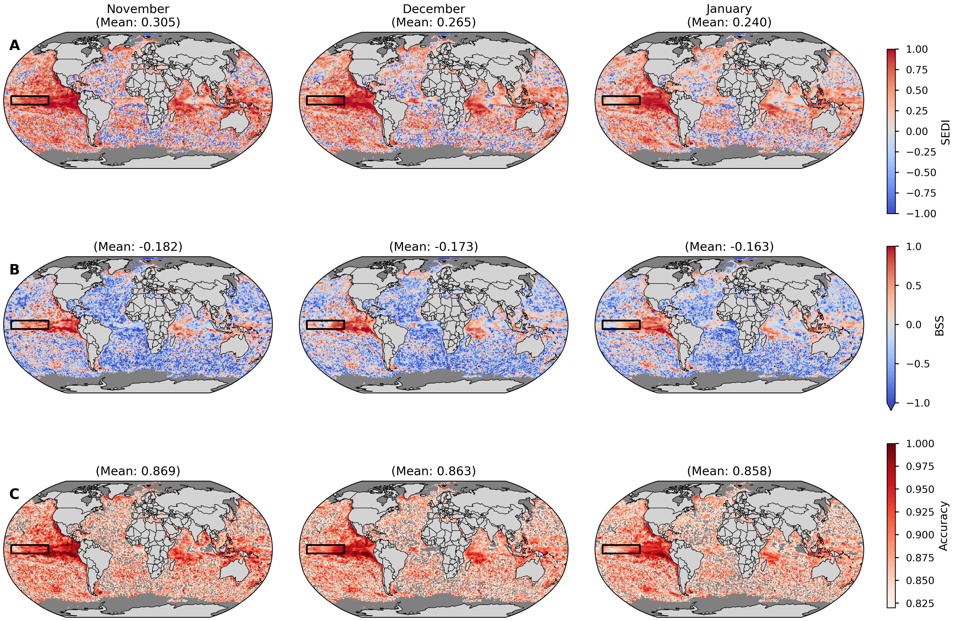
../_images/0fa94a15-3175-4725-863a-fc42e5bcb6c5.png — Fig. 4.1.1 Figure 1: Spatial Forecast Skill for November-December-January (NDJ) Upper Ocean Heatwaves (1993–2023). Skill of Météo-France System-9 forecasts (with nominal start date October 1st) verified against ORAS5 reanalysis. Heatwaves are defined as upper 300m ocean heat content (OHC) anomalies exceeding the 90th percentile within the 1993-2023 period. Rows show: (A) Symmetric Extremal Dependence Index (SEDI), (B) Brier Skill Score (BSS); and (C) Accuracy. In all maps, red areas indicate positive skill (forecast is better than the reference), while blue areas indicate negative skill. Masked areas are shown in grey. For the Accuracy maps (C) the areas with an accuracy lower than what would be expected by random chance (82%) are also shown with a grey color.#

📋 Methodology#

The following steps were applied to evaluate the skill of the seasonal forecasting system in predicting heatwave extremes:

1. Data Preparation

This section includes:

imports, settings, parameter definitions, and reusable functions required to initialize the analysis. Here the extent of the Nino3.4 area is given (5°N–5°S, 170°–120°W, also delineated in most map plots, e.g. Figure 3). This area is selected to represent the tropical Pacific and ENSO, providing a key benchmark for seasonal predictability. The data is also loaded in this section.
Météo-France System-9: The seasonal forecast data includes monthly depth-averaged potential temperature for the upper 300m. We use the hindcasts with a nominal start date of October 1st, between 1993 and 2023. For consistency only the hindcast period is used, since the model system has a different number of ensemble members in the forecast period compared to the hindcast period. depth_average_potential_temperature_of_upper_300m (\(\bar{\Theta}\)) was converted to OHC using the similar constants as used by ORAS5 (pers. comm.): \(\text{OHC} =\rho \, c_p \, \bar{ \Theta} \, dz \), where \( \rho = 1026 \, \text{kg/m}^3\), \( c_p = 3991 \, \text{J/kg/K} \), and \( dz = 300 \, \text{m} \).
ORAS5: Reanalysis OHC for the upper 300m is used as the observational reference. Data is regridded to a common 1° spatial resolution using conservative normalization in xESMF.
The seasonal forecast and reanalysis data were processed for the period from 1993 to 2023; and we consider forecasts with a nominal start date October 1st, valid for November, December, and January. For instance, the last season considers forecasts with a nominal start date October 1st 2023 for November and December 2023, and January 2024. By choosing an October initialization, we avoid compounding the task of extreme event detection with the lower predictability associated with other initialization windows, such as the boreal spring period in the Eastern Tropical Pacific (Jacox et. al. 2022, [1]).
Anomalies: Monthly anomalies are calculated by subtracting the calendar month climatology.
We also apply a common land mask to the interpolated products, also omitting areas where at any time the seasonal forecasts has temperatures below 0°C (we could have used a lower threshold than 0°C, but use this threshold as it at least will mask out all ice covered areas).
The seasonal forecast system (System 9) is initialized by nudging the ocean and sea-ice models towards the Mercator Ocean International GLORYS12V1 reanalysis, except for wihtin 225 km of coastlines or in the presence of sea ice (Specq et. al. 2024, [3]). In contrast, ORAS5 is used as the reference reanalysis in this study. This makes the reference data somewhat independent, however, the data assimilated in ORAS5 and GLORYS12 likely overlap to a great extent. Differences in means will not affect the conclusions as anomalies are considered. Further, the limits for a heatwave is calculated separately for the seasonal forecast data and the reference data, allowing them to have different distributions.

2. OHC Time Series and Trend Analysis

We compare the data in map plots and in area aggregated time-series plots. Initial inspection showed strong temporal trends in OHC during the time period. The linear trends were removed from the raw data, so that the trends would not inflate the skill scores. Further, the strong temporal trends would skew the diagnosis of heatwaves to primarily occur in the more recent years.

3. Model Performance vs. Reanalysis

The OHC anomalies based on detrended data were used to assess heatwaves. We show that the reference data and seasonal forecasting data have different data distributions. To align our diagnosed heatwaves, the defined percentiles of a heatwave are calculated separately depending on both the data source and the calendar month. To avoid unrealistic jumps, and to align our analysis with Jacox et. al. 2022, [1] we use a three-month centered rolling window to set the monthly heatwave thresholds. For instance, January thresholds are derived from pooled December, January, and February anomalies. Heatwaves are defined as anomalies exceeding the 90th percentile.

In the subsequent sections we evaluate the forecast over different dimensions:

Pooling and grouping strategies#

Analysis Goal	Grouping Strategy	Question It Answers
Skill Maps	Pool time and ensemble for each grid point.	“What is the forecast skill at this specific location over the entire 30-year period?”
Annual Time Series	Pooled horizontally and over the ensemble for each year.	“What was the overall global forecast accuracy in the year 1997?”
Summary Tables	Pool time, space, and ensemble for each lead-time (month).	“What was the overall global forecast skill for all Novembers combined in the record?”

4. Metrics: SEDI, BSS, Accuracy

We evaluate the forecasting system using the metrics outlined below.

SEDI - the Symmetric Extremal Dependence Index#

SEDI quantifies the forecast skill for rare binary events (e.g., heatwaves). It is the Symmetric Extremal Dependence Index (Ferro & Stephenson 2011 [4]). SEDI has a maximum value of one, and a minimum value of -1. Scores above zero indicate a forecast better than random chance.

SEDI is built on the output of a contingency table. A contingency table provides: sample size, n; base rate, p; hit rate, H; and false-alarm rate, F. The ensemble members are pooled and each adds to the counts in the contingency table before the SEDI score is calculated.

	Event observed	Non-event observed
Event forecasted	a = Hpn	b = F(1-p)n	a + b
Non-event forecasted	c = (1-H)pn	d = (1-F)(1-p)n	c + d
Sum	a + c = pn	b + d = (1-p)n	n

Hit rate (H) = \( \frac{a}{a+c} \), False alarm rate (F) = \( \frac{b}{b+d} \)

SEDI = \( \frac{logF - logH -log(1-F) + log(1-H)}{logF + logH +log(1-F) + log(1-H)} \)

The Brier Skill Score (BSS)#

The Brier Skill Score (BSS) compares the forecast skill against a reference forecast (e.g., climatology), which for heatwaves defined as values above 90% of those observed, would be that there always was about a 10% chance of a heatwave.

It is calculated as: \( \text{BSS} = 1 - \frac{\text{Brier Score (BrS)}}{\text{BrS}_{\text{ref}}} \)

It is based on the Brier Score, which measures the mean squared error between forecast probabilities and observed binary events.

The BSS’s upper limit is 1, meanwhile it has no lower limit. Scores above zero indicate a forecast better than the climatology, which is around a 10% chance.

Accuracy#

Accuracy measures the proportion of correct predictions (both true positives and true negatives) out of the total number of forecasts made. The formula is:

\( \text{Accuracy} = \frac{\text{True Positives (TP)} + \text{True Negatives (TN)}}{\text{Total Predictions (N)}} \)

For rare events like heatwaves (which occur about 10 % of the time in this study), a simple accuracy score can be misleading. A forecast that always predicts “no heatwave” would be 90 % accurate but have zero skill. Therefore, we compare the forecast’s accuracy to a random chance benchmark. For an event with a 10% probability (p=0.1), the accuracy of a random forecast is calculated as:

\( \text{Random Accuracy} = p^2+(1−p)^2 = 0.1^2+(0.9)^2 = 0.82 \)

This means the forecasting system must achieve an accuracy greater than 0.82 (or 82%) to be considered more skillful than random chance.

5. Contingency Table Analysis The contingency tables for all November, December, and January’s are presented and discussed.

6. Annual Variability and ENSO Influence Finally, we display the annual metrics as time-series, also showing the components of the contingency table, allowing a discussion of the components of the metrics.

Summary of Results

📈 Analysis and results#

1. Data Preparation#

This section includes imports, settings, parameter definitions, and reusable functions required to initialize the analysis.

Imports and Settings#

Definition of Parameters#

We have chosen Meteo-France System-9, and focus on the hindcast period, which are available from 1993 until 2024, to have a consistent ensemble throughout the analysis.

We focus on the forecasts initiated October 1st every year, and consider one, two, and three months leadtimes - i.e. the forecasted values for November, December, and January. In the initial processing also October and February values are used, as the heatwave thresholds are centered a three-month month moving window.

Helper Functions for Data Processing and Plotting#

Show code cell source

Hide code cell source

# map plot helper
def setup_map_plot(ax):
    """
    Applies consistent styling to a Cartopy map axes.
    - Sets the ocean color to gray.
    - Adds land, coastlines, and borders.
    """
    ax.set_facecolor('gray')
    ax.add_feature(cartopy.feature.LAND, facecolor='lightgrey', zorder=2)
    ax.add_feature(cartopy.feature.COASTLINE, linewidth=0.5, zorder=3)
    ax.add_feature(cartopy.feature.BORDERS, linewidth=0.5, zorder=3)
    ax.plot([Nino_3_4_lon[0],Nino_3_4_lon[0],Nino_3_4_lon[1],Nino_3_4_lon[1],Nino_3_4_lon[0]],
                [Nino_3_4_lat[0],Nino_3_4_lat[1],Nino_3_4_lat[1],Nino_3_4_lat[0],Nino_3_4_lat[0]], 
            c='k',transform=ccrs.PlateCarree()) 
    
    
def add_bounds(ds):
    # From https://github.com/COSIMA/ocean-regrid/blob/master/nemo_grid.py
    url = (
        "https://icdc.cen.uni-hamburg.de/thredds/fileServer/ftpthredds/"
        "EASYInit/oras5/ORCA025/mesh/mesh_mask.nc"
    )
    known_hash = "ba88418bc8055972b675ceedbd4345b3827f0ede8cef04d53c97b66a5c7a46a7"
    fname = pooch.retrieve(url, known_hash)
    dg = xr.open_dataset(fname, chunks={}).isel(t=0, z=0)

    # These are the top righ-hand corner of t cells.
    glamf = dg.glamf
    gphif = dg.gphif

    # Extend south so that Southern most cells can have bottom corners.
    gphif_new = np.ndarray((gphif.shape[0] + 1, gphif.shape[1] + 1))
    gphif_new[1:, 1:] = gphif[:]
    gphif_new[0, 1:] = gphif[0, :] - abs(gphif[1, :] - gphif[0, :])

    glamf_new = np.ndarray((glamf.shape[0] + 1, glamf.shape[1] + 1))
    glamf_new[1:, 1:] = glamf[:]
    glamf_new[0, 1:] = glamf[0, :]

    # Repeat first longitude so that Western most cells have left corners.
    gphif_new[:, 0] = gphif_new[:, -1]
    glamf_new[:, 0] = glamf_new[:, -1]

    gphif = gphif_new
    glamf = glamf_new

    # Corners of t points. Index 0 is bottom left and then
    # anti-clockwise.
    clon = np.empty((dg.tmask.shape[0], dg.tmask.shape[1], 4))
    clon[:] = np.nan
    clon[:, :, 0] = glamf[0:-1, 0:-1]
    clon[:, :, 1] = glamf[0:-1, 1:]
    clon[:, :, 2] = glamf[1:, 1:]
    clon[:, :, 3] = glamf[1:, 0:-1]
    assert not np.isnan(np.sum(clon))

    clat = np.empty((dg.tmask.shape[0], dg.tmask.shape[1], 4))
    clat[:] = np.nan
    clat[:, :, 0] = gphif[0:-1, 0:-1]
    clat[:, :, 1] = gphif[0:-1, 1:]
    clat[:, :, 2] = gphif[1:, 1:]
    clat[:, :, 3] = gphif[1:, 0:-1]
    assert not np.isnan(np.sum(clat))

    ds["latitude"].attrs["bounds"] = "latitude_bounds"
    ds["longitude"].attrs["bounds"] = "longitude_bounds"
    return ds.assign_coords(
        latitude_bounds=(["y", "x", "bound"], clat),
        longitude_bounds=(["y", "x", "bound"], clon),
    )


# Seasonal

def preprocess_seasonal(ds):
    """
    New preprocessing function:
    1. Swaps 'leadtime' dimension for 'time' coordinate.
    2. Cleans up metadata (bnds, realization).
    """
    
    # Check if 'leadtime' is a dim, 'time' is a coord, 
    # and 'time' is indexed by 'leadtime'.
    if 'leadtime' in ds.dims and 'time' in ds.coords and 'leadtime' in ds['time'].dims:
        ds = ds.swap_dims({'leadtime': 'time'})

    # Set 'bnds' variables as coordinates
    bnd_vars = [var for var, da in ds.data_vars.items() if "bnds" in da.dims]
    if bnd_vars:
        ds = ds.set_coords(bnd_vars)
        
    # Clean up 'realization' coordinate and ensure it's a dimension
    if 'realization' in ds.coords:
        ds["realization"] = ds["realization"].str.replace(" ", "").astype(str)
        if 'realization' not in ds.dims:
            ds = ds.expand_dims("realization")
            
    return ds

    
def regrid_reanalysis(ds, grid_request, **xesmf_kwargs):
    ds_seasonal = download.download_and_transform(
        *grid_request,
        preprocess=preprocess_seasonal,
        invalidate_cache=False,
        decode_timedelta=False,
    )
    mask_out = (
        ds_seasonal["thetaot300"]
        .isel(
            {dim: 0 for dim in ("realization", "time")}
        )
        .reset_coords(drop=True)
        .notnull()
    )
    grid_out = ds_seasonal.cf[["latitude", "longitude"]].assign_coords(mask=mask_out)

    mask_in = ds["sohtc300"].isel(time=0).reset_coords(drop=True).notnull()
    ds = add_bounds(ds).assign_coords(mask=mask_in)
    return diagnostics.regrid(ds, grid_out, **xesmf_kwargs)
    
def compute_anomalies_new(ds, realizations, grid_request, detrend, **xesmf_kwargs):
    """
    Computes standard monthly anomalies and detrends them 
    month-by-month using a mean-preserving method.
    """
    if realizations is not None:
        ds = ds.isel(realization=realizations)

    if grid_request is not None:
        ds = regrid_reanalysis(ds, grid_request, **xesmf_kwargs)
    else:
        assert not xesmf_kwargs

    ((name, da),) = ds.data_vars.items()
    time_dim = "time"
    
    with xr.set_options(keep_attrs=True):
        
        # --- Standard Monthly Climatology ---
        dims_to_mean = [time_dim]
        if "realization" in da.dims:
            dims_to_mean.append("realization")

        # Calculate mean for each month (Jan, Feb, etc.)
        climatology = da.groupby(f"{time_dim}.month").mean(dim=dims_to_mean)
        
        # Calculate Anomalies
        anomalies = da.groupby(f"{time_dim}.month") - climatology
        
        # --- Month-by-Month Detrending ---
        if detrend:
            # 1. Group by month and fit trend using .map()
            pf_ds = anomalies.groupby(f"{time_dim}.month").map(
                lambda x: x.polyfit(dim=time_dim, deg=1)
            )
            
            # Extract the coefficients DataArray. 
            coeff_name = list(pf_ds.data_vars)[0]
            coeffs = pf_ds[coeff_name]
            
            # Reconstruct the full trend line (mx + c)
            coeffs_expanded = coeffs.sel(month=anomalies[time_dim].dt.month)
            full_trend = xr.polyval(anomalies[time_dim], coeffs_expanded)
            
            # Isolate the slope component.
            slope_component = full_trend - full_trend.mean(dim=time_dim)
            
            # Subtract the slope
            anomalies = anomalies - slope_component

    anomalies.encoding["chunksizes"] = tuple(
        1 if dim == "realization" else size
        for dim, size in anomalies.sizes.items()
    )
    return anomalies.to_dataset(name=name)
    
    
def transform_seasonal_data(ds, realizations, detrend, grid_request, **xesmf_kwargs):
    """
    1. Compute the anomalies
    2. Reindexe the data using reindex_seasonal.
    """
    static_not_sea_ice_proxy_mask_s = (
    (ds['thetaot300'] > 273.15) # 
    .all(dim=['time', 'realization']) # 
    )
    static_not_sea_ice_proxy_mask_s = static_not_sea_ice_proxy_mask_s.compute()

    #print(f"Number of 'True' points in sesonal static_sea_ice_proxy_mask: {static_not_sea_ice_proxy_mask_s.sum().compute().item()}")
    #static_not_sea_ice_proxy_mask_s.plot()
    # Step 1: Compute anomalies
    ds_anom = compute_anomalies_new(
        ds,
        realizations=realizations,
        detrend=detrend,
        grid_request=grid_request,
        **xesmf_kwargs
    )
    #apply the mask here
    xr.set_options(keep_attrs=True)
    ds_anom['thetaot300'] = ds_anom['thetaot300'].where(static_not_sea_ice_proxy_mask_s)

    ds_anom = ds_anom.load()
    # --------------------------

    # Step 2: Reindex to (year, month), assing year to fc_start
    ds_reindexed = reindex_seasonal(
        ds_anom, 
        time_dim='time', 
        shift_months=[1, 2, 3, 4] 
    )
    
    return ds_reindexed

def transform_reanalysis_data(ds, realizations, detrend, grid_request, **xesmf_kwargs):
    """
    Wrapper function to process reanalysis data:
    1. Compute anomalies 
    2. Reindexe the data using a fixed seasonal function.
    """

    # Step 1: Compute anomalies
    ds_anom = compute_anomalies_new(  
        ds,
        realizations=realizations,
        detrend=detrend,
        grid_request=grid_request,
        **xesmf_kwargs
    )

    ds_anom = ds_anom.load() 
    # --------------------------

    months_to_shift = [1, 2, 3, 4] 
    ds_reindexed = reindex_seasonal(
        ds_anom, 
        time_dim='time', 
        shift_months=months_to_shift 
    )
    
    return ds_reindexed

    

def reindex_seasonal(ds, time_dim='time', shift_months=[1, 2, 3, 4]):
    """
    Reindexes to (year, month) by shifting specified months.
    Assign all the fc months to the initialization year
    """
    calendar_year = ds[time_dim].dt.year
    calendar_month = ds[time_dim].dt.month
    
    # Create the 'season_year'
    season_year = xr.where(
        calendar_month.isin(shift_months),
        calendar_year - 1,
        calendar_year
    )
    
    ds = ds.assign_coords(
        season_year=('time', season_year.data), 
        month=('time', calendar_month.data)
    )
    
    ds = ds.set_index(time=("season_year", "month")).unstack("time")
    ds = ds.rename({'season_year': 'year'})
    
    # the month coord will be [1, 2, 3, 4, 10, 11, 12]
    return ds

Data Loading#

We download the reanalysis and seasonal forecast datasets, regridding the reanalysis data to align with the seasonal forecast grid, and computing the detrended anomalies. These transformations are performed using the c3s_eqc_automatic_quality_control download.download_and_transform function and custom preprocessing steps. xesmf conservative regridding was used to transform the ORAS5 ORCA025 grid to a global 1x1 latlon grid. Sensitivity tests were conducted to ensure that the regridding process (comparing area-conservative interpolation used for ORAS5 vs. a version of the two step distance-weighted interpolation that System 9 underwent) produced similar changes to the mean and variance of the original data (not shown).

The data is combined and reindexed so that year and calendar month are the dataset coordinates.
The long-term climatology and possibly the monthly trend is subtracted.
We apply a common land mask and also mask out areas where seasonal forecast data have values corresponding to a monthly mean potential temperature below 0°C.
The seasonal forecast vertically integrated potential temperature is converted to OHC, following the convention used in ORAS5.
The variable names are changed to reflect their current state.

Show code cell source

Hide code cell source

collection_id_reanalysis = "reanalysis-oras5"
collection_id_seasonal = "seasonal-monthly-ocean"

#requests_reanalysis = {leadtime: [] for leadtime in leadtimes}
requests_seasonal = []
for date in pd.date_range(start, stop, freq=freq):
    requests_seasonal.append(
        {
            "originating_centre": "meteo_france",
            "system": "9",
            "variable": ["depth_average_potential_temperature_of_upper_300m"],
            "forecast_type": ["hindcast"],
            "year": date.strftime("%Y"),
            "month": date.strftime("%m"),
        }
    )


print("Building a flat list of unique reanalysis requests...")
requests_reanalysis_flat = []
seen_requests = set() # To prevent duplicate requests

for date in pd.date_range(start, stop, freq=freq):
    for leadtime in leadtimes:
        date_reanalysis = date + pd.DateOffset(months=leadtime)
        request = {
            "product_type": [
                "operational" if date_reanalysis.year > 2014 else "consolidated"
            ],
            "vertical_resolution": "single_level",
            "variable": ["ocean_heat_content_for_the_upper_300m"],
            "year": date_reanalysis.strftime("%Y"),
            "month": date_reanalysis.strftime("%m"),
        }
        request_key = (request["year"], request["month"])
        if request_key not in seen_requests:
            requests_reanalysis_flat.append(request)
            seen_requests.add(request_key)

print(f"Found {len(requests_reanalysis_flat)} unique months of reanalysis to download.")

# Seasonal
ds_seasonal_trend = download.download_and_transform(
    collection_id_seasonal,
    requests_seasonal,
    preprocess=preprocess_seasonal,
    drop_variables="hcrs",
    transform_func=transform_seasonal_data,
    invalidate_cache=False,
    transform_func_kwargs={
        "realizations": realizations,
        "detrend": False,
        "grid_request": None,
    },
    transform_chunks=False,
    decode_timedelta=False,
)
ds_seasonal_trend = ds_seasonal_trend.chunk({
    'year': -1, 
    'month': -1, 
    'realization': 1  
}).astype(np.float32)

# Seasonal
ds_seasonal = download.download_and_transform(
    collection_id_seasonal,
    requests_seasonal,
    preprocess=preprocess_seasonal,
    drop_variables="hcrs",
    transform_func=transform_seasonal_data,
    invalidate_cache=False,
    transform_func_kwargs={
        "realizations": realizations,
        "detrend": True,
        "grid_request": None,
    },
    transform_chunks=False,
    decode_timedelta=False,
)

ds_seasonal = ds_seasonal.chunk({
    'year': -1, 
    'month': -1, 
    'realization': 1 
}).astype(np.float32)


# Reanalysis
ds_reanalysis_trend = download.download_and_transform(
    collection_id_reanalysis,
    requests_reanalysis_flat,  
    transform_func=transform_reanalysis_data, 
    invalidate_cache=False,
    drop_variables="time_counter_bnds",
    transform_func_kwargs={
        "realizations": None,  
        "detrend": False,
        "grid_request": (collection_id_seasonal, requests_seasonal[0]),
        "method": "conservative_normed",
        "periodic": True,
        "ignore_degenerate": True,
    },
    transform_chunks=False,
)

ds_reanalysis_trend = ds_reanalysis_trend.chunk({'year': -1, 'month': -1}).astype(np.float32)

ds_reanalysis = download.download_and_transform(
    collection_id_reanalysis,
    requests_reanalysis_flat,  
    transform_func=transform_reanalysis_data, 
    invalidate_cache=False,
    drop_variables="time_counter_bnds",
    transform_func_kwargs={
        "realizations": None, 
        "detrend": True,
        "grid_request": (collection_id_seasonal, requests_seasonal[0]),
        "method": "conservative_normed",
        "periodic": True,
        "ignore_degenerate": True,
    },
    transform_chunks=False,
)
ds_reanalysis = ds_reanalysis.chunk({'year': -1, 'month': -1}).astype(np.float32)

# post processing: conversion and applying the common mask 
# (the seas fc has an additional mask now, removing cold areas, 
# computed before converted to anomalies )
mask1 = ds_reanalysis['sohtc300'].isel(month=1, year=1).isnull()
mask2 = ds_seasonal['thetaot300'].isel(month=1, year=1, realization=0).isnull()

landice_mask=mask1.where((mask1<1) & (mask2 <1) )+1

comask = landice_mask.compute()

# convert the seasonal values to potential temperature expressed as OHC
ds_seasonal = ds_seasonal * heat_content_factor
ds_seasonal_trend = ds_seasonal_trend * heat_content_factor
# reaname the variables

ds_seasonal = ds_seasonal.rename({'thetaot300': 'sohtc300_anomalies'})
ds_reanalysis_trend = ds_reanalysis_trend.astype(np.float32)
ds_seasonal_trend = ds_seasonal_trend.rename({'thetaot300': 'sohtc300_anomalies'})
ds_reanalysis = ds_reanalysis.rename({'sohtc300': 'sohtc300_anomalies'})
ds_reanalysis_trend = ds_reanalysis_trend.rename({'sohtc300': 'sohtc300_anomalies'})

#add inn the common mask again, also using an ice-proxy from the seasonal fc data
xr.set_options(keep_attrs=True)
ds_seasonal['sohtc300_anomalies'] = ds_seasonal['sohtc300_anomalies']*comask
ds_seasonal_trend['sohtc300_anomalies'] = ds_seasonal_trend['sohtc300_anomalies']*comask
ds_reanalysis['sohtc300_anomalies'] = ds_reanalysis['sohtc300_anomalies']*comask
ds_reanalysis_trend['sohtc300_anomalies'] = ds_reanalysis_trend['sohtc300_anomalies']*comask

Building a flat list of unique reanalysis requests...
Found 155 unique months of reanalysis to download.

2. OHC Time Series and Trend Analysis#

Compares the model’s OHC and heatwave representation against the reanalysis. The time series of globally averaged OHC anomalies clearly shows a strong positive trend over the 1993-2023 period (Figure 2). This warming trend is present in both the ORAS5 reanalysis and the Météo-France System 9 seasonal forecasts, though it is slightly stornger in Météo-France System 9. Because this predictable, long-term signal could artificially inflate skill scores, the linear trend is removed from both datasets for all subsequent heatwave and skill analyses. The detrended time series shows the interannual variability, such as the strong El Niño events, more clearly.

Show code cell source

Hide code cell source

# Time series plotting
def plot_regional_timeseries(seasonal_da, reanalysis_da, nino_box, trend_status=""):
    """Generates a 2-panel plot of global and Nino3.4 time series."""
    
    month_order = [11, 12, 1] 
    month_names = ['Nov', 'Dec', 'Jan']
    month_map = {11: 'Nov', 12: 'Dec', 1: 'Jan'}
    
    # Sort the data 
    seasonal_da = seasonal_da.sel(month=month_order)
    reanalysis_da = reanalysis_da.sel(month=month_order)
    weights = np.cos(np.deg2rad(reanalysis_da['latitude'])).astype(np.float32)
    weights.name = "weights"
    
    # Perform the mean operations (using ensemble mean for forecast)
    s_global = seasonal_da.weighted(weights).mean(['latitude', 'longitude'])
    r_global = reanalysis_da.weighted(weights).mean(['latitude', 'longitude'])
    s_nino = seasonal_da.sel(**nino_box).weighted(weights).mean(['latitude', 'longitude'])
    r_nino = reanalysis_da.sel(**nino_box).weighted(weights).mean(['latitude', 'longitude'])

    # --- Compute Monthly Correlations ---
    # We take the ensemble mean of the forecast first, then correlate with reanalysis per month
    s_global_mean = s_global.mean('realization')
    s_nino_mean = s_nino.mean('realization')

    # This produces a correlation value for each month [11, 12, 1]
    corr_global_monthly = xr.corr(r_global, s_global_mean, dim='year').compute()
    corr_nino_monthly = xr.corr(r_nino, s_nino_mean, dim='year').compute()

    # Format the correlation strings for the title
    def format_corr_str(corr_da):
        return ", ".join([f"{month_map[m]}: {corr_da.sel(month=m).item():.2f}" for m in month_order])

    title_global = f"Global Mean | r = {format_corr_str(corr_global_monthly)}"
    title_nino = f"Niño 3.4 Region | r = {format_corr_str(corr_nino_monthly)}"

    # --- Plotting ---
    fig, axs = plt.subplots(2, 1, figsize=(16, 10), sharex=True)
    plt.suptitle(f"NDJ OHC Anomalies ({trend_status}) - Forecasts vs. ORAS5 (bold)", fontsize=16)

    # Convert to DataFrames for seaborn
    s_global_df = s_global.to_dataframe(name='anomaly').reset_index() 
    r_global_df = r_global.to_dataframe(name='anomaly').reset_index()
    s_nino_df = s_nino.to_dataframe(name='anomaly').reset_index()
    r_nino_df = r_nino.to_dataframe(name='anomaly').reset_index()

    for df in [s_global_df, r_global_df, s_nino_df, r_nino_df]:
        df['month_name'] = pd.Categorical(df['month'].map(month_map), categories=month_names, ordered=True)

    # Panel 0: Global
    sns.stripplot(data=s_global_df, x="year", y="anomaly", hue="month_name", dodge=True, alpha=.3, legend=False, palette="muted", ax=axs[0])
    sns.stripplot(data=r_global_df, x="year", y="anomaly", hue="month_name", ax=axs[0], palette="dark", dodge=True, linewidth=1, edgecolor="white")
    axs[0].set_title(title_global, fontsize=14)
    axs[0].axhline(0, color="k", lw=0.8, ls="--")
    axs[0].set_ylabel("OHC Anomaly [J/m²]")

    # Panel 1: Nino 3.4
    sns.stripplot(data=s_nino_df, x="year", y="anomaly", hue="month_name", dodge=True, alpha=.3, legend=False, palette="muted", ax=axs[1])
    sns.stripplot(data=r_nino_df, x="year", y="anomaly", hue="month_name", ax=axs[1], palette="dark", dodge=True, linewidth=1, edgecolor="white")
    axs[1].set_title(title_nino, fontsize=14)
    axs[1].axhline(0, color="k", lw=0.8, ls="--")
    axs[1].set_ylabel("OHC Anomaly [J/m²]")
    
    plt.xticks(rotation=45)
    plt.tight_layout(rect=[0, 0, 1, 0.95])

# --- Execute plotting ---
ds_s_trend_ndj = ds_seasonal_trend['sohtc300_anomalies']
ds_r_trend_ndj = ds_reanalysis_trend['sohtc300_anomalies']

ds_s_trend_ndj = ds_s_trend_ndj.chunk({'year': -1, 'month': -1, 'realization': 1})
ds_r_trend_ndj = ds_r_trend_ndj.chunk({'year': -1, 'month': -1})
 
plot_regional_timeseries(ds_s_trend_ndj, ds_r_trend_ndj, nino_box, trend_status="With Trend")

gc.collect();

ds_s_ndj = ds_seasonal['sohtc300_anomalies']
ds_r_ndj = ds_reanalysis['sohtc300_anomalies']

ds_s_ndj = ds_s_ndj.chunk({'year': -1, 'month': -1, 'realization': 1})
ds_r_ndj = ds_r_ndj.chunk({'year': -1, 'month': -1})

plot_regional_timeseries(ds_s_ndj, ds_r_ndj, nino_box, trend_status="Detrended")

gc.collect();

../_images/1e9e4ccaac16dd7888fd4bd49cd9c56446c689edcd92a363f537eed68150ffc7.png

../_images/c1a1d20ffdaa232c22d578caaea8d14f87f526c7ebdb0a0a0f88b35b7973f45b.png

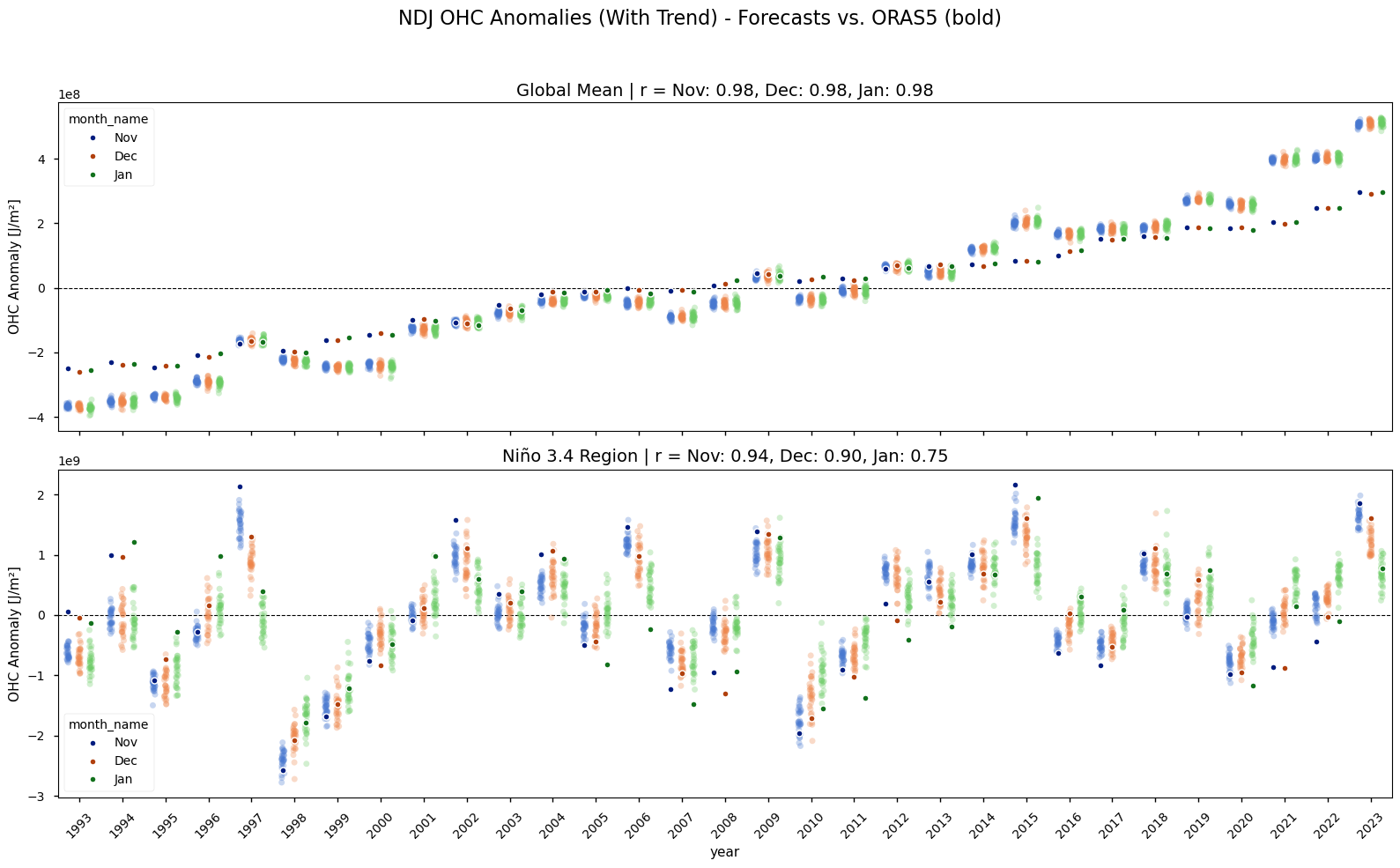
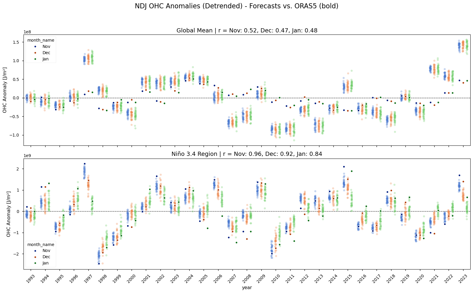
Figure 2#

Annual time series of reanalysis and forecast anomalies according to calendar month. The forecast fields have a nominal start date October 1st. The single dots with a stronger color shows the reanalysis data, while the more lightly colored plot clouds show the seasonal forecasts (one dot per realization). The upper two rows show the anomalies in the original time-series for the global and Niño3.4 area, while the lower panels show the detrended data. The subplot-titles provide the Pearson correlation coefficients of the area averaged anomalies. Note that the y-axis range varies.

3. Model Performance vs. Reanalysis#

This section directly compares the model’s OHC and heatwave representation against the reanalysis, after having detrended both.

Correlation of OHC Anomalies#

/data/common/miniforge3/envs/wp3/lib/python3.12/site-packages/dask/array/numpy_compat.py:58: RuntimeWarning: invalid value encountered in divide
  x = np.divide(x1, x2, out)

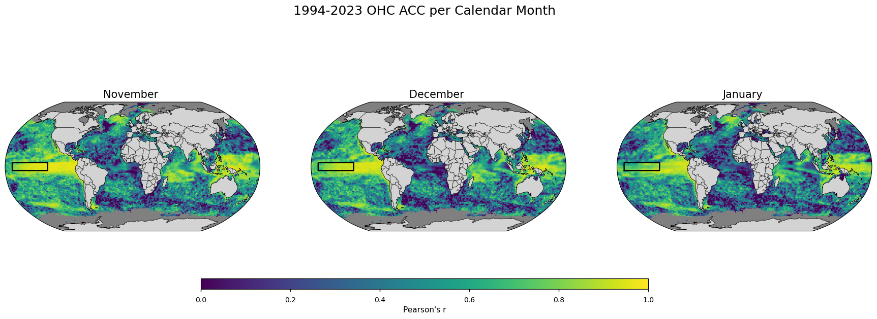
../_images/b46d23453ee10927c05daec19df2f41331e187932b8f62616d39a6d6eba4886f.png

Figure 3#

Map plot showing the temporal anomaly correlation coefficients (Pearson’s) between the forecast ensemble mean and the reanalysis 1993-2023 NDJ OHC every valid grid box.

Comparison of distributions#

We inspect the OHC anomalies in the two data sources to see if they share a similar distribution. We look at November, December, and January simultaneously and pool the seasonal forecast ensemble members. Identical distributions and tails would allow for the use of the same physical magnitudes for a heatwave threshold.

The differences in the probability density functions, the longer tails in the reanalysis versus the more blunt tails in the forecasts justify the use of relative heatwave thresholds depending on the specific data source.

Show code cell source

Hide code cell source

def compare_anomaly_statistics_weighted(ds_seasonal, ds_reanalysis, comask, step=5):
    """
    Compares the distribution of OHC anomalies using area-weighting and subsampling.
    Includes Kurtosis to describe the 'Leptokurtic' (thin) vs 'Platykurtic' (not-thin) 
    nature of the variability tails. 
    The data is spatially subsampled to reduce the computational cost.
    """
    print(f"Starting statistical analysis (subsampling step: {step})...")

    # 1. Data Selection (NDJ) and Masking
    # Selecting late autumn/winter months and applying the common ocean mask
    da_s = ds_seasonal['sohtc300_anomalies'].sel(month=[11, 12, 1]).where(comask.notnull())
    da_r = ds_reanalysis['sohtc300_anomalies'].sel(month=[11, 12, 1]).where(comask.notnull())

    # 2. Spatial Subsampling
    # Compute early to bring data into memory for weighted statistics and quantiles
    da_s_sub = da_s.isel(latitude=slice(0, None, step), longitude=slice(0, None, step)).compute()
    da_r_sub = da_r.isel(latitude=slice(0, None, step), longitude=slice(0, None, step)).compute()

    # 3. Area Weights Calculation
    # Using cosine of latitude to account for grid cell area convergence at poles
    weights = np.cos(np.deg2rad(da_s_sub.latitude))
    
    # Broadcast weights to match the 2D/3D shape of the data for flattening
    weights_s = weights.broadcast_like(da_s_sub)
    weights_r = weights.broadcast_like(da_r_sub)

    # 4. Compute Weighted Statistics
    print("Computing weighted statistics...")
    std_s = da_s_sub.weighted(weights).std().item()
    std_r = da_r_sub.weighted(weights).std().item()

    # Calculate weighted quantiles for the Q-Q plot (focusing on the extreme upper tail)
    q_levels = np.linspace(0.85, 0.99, 50)
    s_quant = da_s_sub.weighted(weights).quantile(q_levels).values
    r_quant = da_r_sub.weighted(weights).quantile(q_levels).values

    # 5. Prepare Data for PDF/Kurtosis (flattening and dropping NaNs)
    s_vals = da_s_sub.values.flatten()
    s_w    = weights_s.values.flatten()
    mask_s = ~np.isnan(s_vals)
    s_vals, s_w = s_vals[mask_s], s_w[mask_s]

    r_vals = da_r_sub.values.flatten()
    r_w    = weights_r.values.flatten()
    mask_r = ~np.isnan(r_vals)
    r_vals, r_w = r_vals[mask_r], r_w[mask_r]

    # Calculate Fisher Kurtosis (Normal distribution = 0)
    # Positive = Leptokurtic (fat tails), Negative = Platykurtic (thin tails)
    kurt_s = stats.kurtosis(s_vals)
    kurt_r = stats.kurtosis(r_vals)

    # Kolmogorov-Smirnov test (unweighted) to check if distributions are identical
    ks_stat, ks_p = stats.ks_2samp(s_vals, r_vals)

    # Calculate the number of ensemble members
    n_members = len(ds_seasonal.realization)
    
    # Calculate points per realization for the forecast
    points_per_member = len(s_vals) / n_members

    # Printing Results Table
    stats_df = pd.DataFrame({
        'Metric': ['StdDev (J/m²)', 'Kurtosis', 'Total Points', 'Points per Member'],
        'Forecast (S9)': [f"{std_s:.2e}", f"{kurt_s:.2f}", len(s_vals), int(points_per_member)],
        'Reanalysis (ORAS5)': [f"{std_r:.2e}", f"{kurt_r:.2f}", len(r_vals), len(r_vals)]
    })

    print("\n--- Statistics Summary ---")
    print(stats_df.to_string(index=False))
    print(f"K-S Test p-value: {ks_p:.2e}")

    # 7. Visualization
    fig, (ax1, ax2) = plt.subplots(1, 2, figsize=(18, 7))
    
    # Left: Area-Weighted Probability Density Function (KDE)
    sns.kdeplot(x=s_vals, weights=s_w, ax=ax1, label='Forecast (System 9)', color='blue', fill=True, alpha=0.3)
    sns.kdeplot(x=r_vals, weights=r_w, ax=ax1, label='Reanalysis (ORAS5)', color='red', fill=True, alpha=0.3)
    ax1.set_title(f"Area-Weighted Anomaly PDFs", fontsize=14)
    ax1.set_xlabel("OHC Anomaly [J/m²]")
    ax1.legend()
    
    # Right: Q-Q Plot for the Upper Tail Comparison
    ax2.plot(r_quant, s_quant, 'ko-', markersize=4, label='Weighted Quantiles')
    ax2.plot([min(r_quant), max(r_quant)], [min(r_quant), max(r_quant)], 'r--', label='1:1 Line')
    ax2.set_title("Upper Tail Comparison (85th to 99th percentile)", fontsize=14)
    ax2.set_xlabel("Reanalysis Quantiles [J/m²]")
    ax2.set_ylabel("Forecast Quantiles [J/m²]")
    ax2.grid(True, alpha=0.3)
    ax2.legend()
    
    plt.tight_layout()
    plt.show()

# Execution call
compare_anomaly_statistics_weighted(ds_seasonal, ds_reanalysis, comask=comask, step=5)

Starting statistical analysis (subsampling step: 5)...
Computing weighted statistics...

--- Statistics Summary ---
           Metric Forecast (S9) Reanalysis (ORAS5)
    StdDev (J/m²)      6.40e+08           6.71e+08
         Kurtosis          4.18               6.50
     Total Points       3687357             118947
Points per Member        118947             118947
K-S Test p-value: 1.73e-47

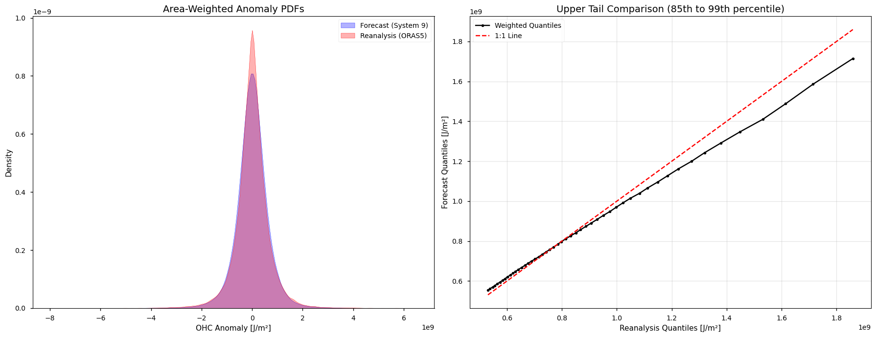
../_images/3dc66e2cf7d4c27583713dd7d66f28638f276855228b25684469875a34d73683.png

Figure 4#

Distribution analysis of pooled OHC anomalies for the NDJ season. The left plot shows the area-weighted probability density functions (PDFs) for the forecast (blue) and reanalysis (red), where the broader “shoulders” of the blue curve indicate a blunter distribution. The right plot shows a quantile-quantile comparison of the upper tail (\(P_{85}\) to \(P_{99}\)) of the two data sources. The black line falling below the diagonal indicate higher intensity values (longer tails) in the reanalysis data compared to the forecast.

Comparison of Heatwave Representation#

Heatwaves are defined as monthly anomalies exceeding a 90th percentile threshold. The thresholds are calculated from a three-month centered moving window, and separately for each data source. For reanalysis data, the threshold is calculated across all years at each grid point. For the seasonal forecast, the threshold is calculated across all years and all ensemble members at each grid point.

Show code cell source

Hide code cell source

def calculate_heatwave_masks(ds_seasonal, ds_reanalysis, comask):
    """
    Calculates binary heatwave masks using a 90th percentile threshold 
    derived from a 3-month centered rolling window.
    """
    
    # --- 1. Data Preparation ---
    da_r = ds_reanalysis['sohtc300_anomalies'].chunk({**spatial_chunks, **time_chunks})
    da_s = ds_seasonal['sohtc300_anomalies'].chunk({**spatial_chunks, 'realization': 1, **time_chunks})

    # --- 2. Threshold Calculation (Centered Windows) ---
    months = [11, 12, 1]
    month_labels = {11: 'Nov ', 12: 'Dec ', 1: 'Jan '}

    # Reanalysis thresholds (ORAS5 reference)
    p90_r_list = [
        da_r.sel(month=[10, 11, 12]).quantile(0.9, dim=['month', 'year'], method="higher"),
        da_r.sel(month=[11, 12, 1]).quantile(0.9, dim=['month', 'year'], method="higher"),
        da_r.sel(month=[12, 1, 2]).quantile(0.9, dim=['month', 'year'], method="higher")
    ]
    p90_r_lazy = xr.concat(p90_r_list, dim='month').assign_coords(month=months)

    # Seasonal Forecast thresholds (System 9)
    p90_s_list = [
        da_s.sel(month=[10, 11, 12]).quantile(0.9, dim=['month', 'year', 'realization']),
        da_s.sel(month=[11, 12, 1]).quantile(0.9, dim=['month', 'year', 'realization']),
        da_s.sel(month=[12, 1, 2]).quantile(0.9, dim=['month', 'year', 'realization'])
    ]
    p90_s_lazy = xr.concat(p90_s_list, dim='month').assign_coords(month=months)

    # Compute p90 values
    print("Computing p90 thresholds...")
    (p90_r, p90_s) = dask_compute(p90_r_lazy, p90_s_lazy)
    print("Thresholds computed.")

    # --- 3. Unified Scaling and Plotting (2x3 Grid) ---
    fig, axs = plt.subplots(
        nrows=2, ncols=3, figsize=(22, 12),
        subplot_kw={'projection': ccrs.Robinson()}
    )
    plt.suptitle("p90 Threshold Comparison: Reanalysis (top) vs. Forecast (bottom)", fontsize=20)
    
    # Unified color limits for all 6 panels to ensure fair comparison
    combined_data = xr.concat([p90_r, p90_s], dim='src')
    vmin, vmax = vmin, vmax = np.nanpercentile(combined_data.values, [2, 98]) 
    
    cmap = plt.get_cmap('viridis')
    weights = np.cos(np.deg2rad(p90_r['latitude']))

    for i, m in enumerate(months):
        # Row 0: Reanalysis Reference (ORAS5)
        ax_r = axs[0, i]
        im = p90_r.sel(month=m).plot(
            ax=ax_r, transform=ccrs.PlateCarree(), cmap=cmap, 
            vmin=vmin, vmax=vmax, add_colorbar=False
        )
        r_mean = p90_r.sel(month=m).weighted(weights).mean().item()
        ax_r.set_title(f"Reanalysis {month_labels[m]}\nGlobal Mean: {r_mean:.2e}")
        setup_map_plot(ax_r)

        # Row 1: Forecast Thresholds (System 9)
        ax_s = axs[1, i]
        p90_s.sel(month=m).plot(
            ax=ax_s, transform=ccrs.PlateCarree(), cmap=cmap, 
            vmin=vmin, vmax=vmax, add_colorbar=False
        )
        s_mean = p90_s.sel(month=m).weighted(weights).mean().item()
        ax_s.set_title(f"Forecast {month_labels[m]}\nGlobal Mean: {s_mean:.2e}")
        setup_map_plot(ax_s)

    # Shared colorbar for all subplots
    cbar_ax = fig.add_axes([0.3, 0.08, 0.4, 0.02])
    fig.colorbar(im, cax=cbar_ax, orientation='horizontal', label='OHC Anomaly [J/m²]')

    plt.subplots_adjust(bottom=0.15, top=0.92, hspace=0.3)

    # --- 4. Mask Generation ---
    fill_value = np.int8(-99)
    da_r_ndj = da_r.sel(month=months)
    da_s_ndj = da_s.sel(month=months)

    print("Generating heatwave masks...")
    masks_s_list = []
    for r in da_s['realization'].values:
        m_s = xr.where(da_s_ndj.sel(realization=r) > p90_s, 1.0, 0.0)
        m_s = m_s.where(comask.notnull()).fillna(fill_value).astype(np.int8).compute()
        masks_s_list.append(m_s.expand_dims(realization=[r]))
        gc.collect()

    heatwave_mask_forecast = xr.concat(masks_s_list, dim='realization')
    
    mask_r_lazy = xr.where(da_r_ndj > p90_r, 1.0, 0.0)
    heatwave_mask_reanalysis = mask_r_lazy.where(comask.notnull()).fillna(fill_value).astype(np.int8).compute()
 
    heatwave_mask_reanalysis.encoding['_FillValue'] = fill_value
    heatwave_mask_forecast.encoding['_FillValue'] = fill_value
    
    return heatwave_mask_forecast, heatwave_mask_reanalysis

# --- Call the function ---
heatwave_mask_forecast, heatwave_mask_reanalysis = calculate_heatwave_masks(
    ds_seasonal,  
    ds_reanalysis,     
    comask
)

# Clean up
gc.collect();

Computing p90 thresholds...

/data/common/miniforge3/envs/wp3/lib/python3.12/site-packages/numpy/lib/_nanfunctions_impl.py:1617: RuntimeWarning: All-NaN slice encountered
  return fnb._ureduce(a,

Thresholds computed.
Generating heatwave masks...

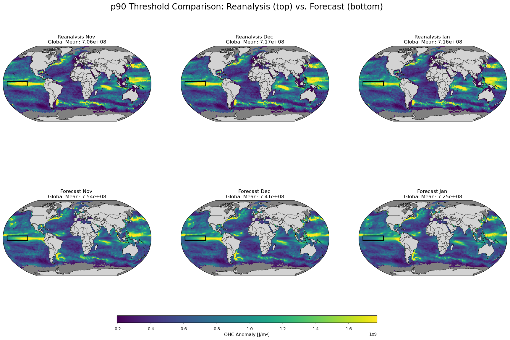
../_images/aa74452e7078d8072ade0acf45346d2e7baac3d59925a34b2e6f988f18149efc.png

Figure 5#

Map plot showing the definition of heatwave (or the grid cell threshold to be exceeded) in the OHC anomalies for the seasonal forecasts (left) and the reanalysis (right).

Diagnostic Plots.#

We choose 1997 as our year to inspect the spatial patterns of the anomalies.

Show code cell source

Hide code cell source

def plot_monthly_anomalies_3x3(ds_seasonal, ds_reanalysis, year):
    """
    Plots a 3x3 grid for a specific year (e.g., 1997).
    Columns: November, December, January
    Rows: Forecast, Reanalysis, Difference
    """
    months = [11, 12, 1]
    month_names = {11: 'November', 12: 'December', 1: 'January'}
    
    # --- 1. Selection & Computation ---
    da_s = ds_seasonal['sohtc300_anomalies'].sel(year=year, month=months).mean('realization')
    da_r = ds_reanalysis['sohtc300_anomalies'].sel(year=year, month=months)
    da_diff = da_s - da_r

    # Bring small spatial slices into memory
    da_s, da_r, da_diff = dask_compute(da_s, da_r, da_diff)

    # --- 2. Figure Setup ---
    fig, axs = plt.subplots(
        nrows=3, ncols=3, figsize=(22, 14),
        subplot_kw={'projection': ccrs.Robinson()}
    )
    plt.suptitle(f"OHC Anomalies: {year} Monthly Progression", fontsize=22, y=0.96)

    cmap = plt.get_cmap('RdBu_r')
    cmap.set_bad(alpha=0)
    
    # Consistent scale for rows 1 & 2
    combined_vals = xr.concat([da_s, da_r], dim='tmp')
    vmin, vmax = np.nanpercentile(combined_vals.values, [2, 98])
    
    # Separate scale for the difference row
    diff_lim = np.nanpercentile(np.abs(da_diff.values), 98)

    # --- 3. Plotting Grid ---
    for i, m in enumerate(months):
        # Row 1: Forecast (Météo-France System 9)
        im_s = da_s.sel(month=m).plot(ax=axs[0, i], transform=ccrs.PlateCarree(), cmap=cmap, 
                                      vmin=vmin, vmax=vmax, add_colorbar=False)
        axs[0, i].set_title(month_names[m], fontsize=16, fontweight='bold')
        if i == 0: axs[0, i].text(-0.07, 0.5, 'Forecast', transform=axs[0, i].transAxes, 
                                  rotation=90, va='center', ha='right', fontsize=16)

        # Row 2: Reanalysis (ORAS5)
        im_r = da_r.sel(month=m).plot(ax=axs[1, i], transform=ccrs.PlateCarree(), cmap=cmap, 
                                      vmin=vmin, vmax=vmax, add_colorbar=False)
        axs[1, i].set_title("") # Keep top title as column header
        if i == 0: axs[1, i].text(-0.07, 0.5, 'Reanalysis', transform=axs[1, i].transAxes, 
                                  rotation=90, va='center', ha='right', fontsize=16)

        # Row 3: Difference (Bias)
        im_d = da_diff.sel(month=m).plot(ax=axs[2, i], transform=ccrs.PlateCarree(), cmap='PuOr', 
                                         vmin=-diff_lim, vmax=diff_lim, add_colorbar=False)
        axs[2, i].set_title("")
        if i == 0: axs[2, i].text(-0.07, 0.5, 'Difference', transform=axs[2, i].transAxes, 
                                  rotation=90, va='center', ha='right', fontsize=16)

    # Styling and horizontal colorbars
    for ax in axs.flat:
        setup_map_plot(ax)
        
    # Positioning colorbars at the bottom
    cbar_ax1 = fig.add_axes([0.15, 0.08, 0.3, 0.02])
    fig.colorbar(im_s, cax=cbar_ax1, orientation='horizontal', label='Anomaly [J/m²]')
    
    cbar_ax2 = fig.add_axes([0.55, 0.08, 0.3, 0.02])
    fig.colorbar(im_d, cax=cbar_ax2, orientation='horizontal', label='Difference [J/m²]')

    plt.subplots_adjust(bottom=0.15, top=0.9, wspace=0.05, hspace=0.15)
    plt.show()

# Run the plot
plot_monthly_anomalies_3x3(ds_seasonal, ds_reanalysis, year=1997)
gc.collect();

../_images/de4af9c5a02c8a4128aad5d1c631bd3d4e6d407cac8e4433b94e54d30f8618a4.png

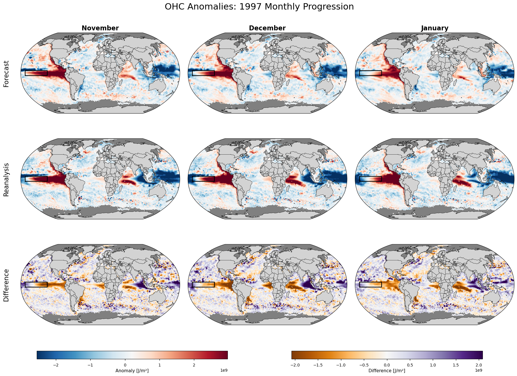
Figure 6#

Map plots showing ensemble mean OHC anomalies from the seasonal forecast with a nomianal start date 1 October 1997 (upper row), the corresponding reanalysis fields (centre row), and their difference (forecast minus reanalysis, bottom row).

4. Metrics: SEDI, BSS, Accuracy#

This section presents the primary skill scores (SEDI, BSS, Accuracy).

Symmetric Extremal Dependence Index (SEDI)#

SEDI (Ferro & Stephenson 2011, [4]) is calculated using the hit rate (H) and false alarm rate (F), as can be found in a contingency table:

\( \text{SEDI} = \frac{\log(F) - \log(H) - \log(1-F) + \log(1-H)}{\log(F) + \log(H) + \log(1-F) + \log(1-H)} \)

To avoid numerical issues, logarithms are computed using a lower bound of \(10^{-6}\).

The Brier Skill Score (BSS)#

The Brier Skill Score (BSS) here compares the forecast’s Brier score against the Brier score of using the climatology of the reference data set as a forecast. The climatologically based heatwave forecast is near a 10% chance, but is here calculated explicitly per grid point. The BSS’s upper limit is 1, meanwhile it has no lower limit. Scores above zero indicate a forecast better than climatology.

Accuracy Assessment#

Proportion of correct predictions relative to total events. Forecast accuracy was calculated as: \( \text{Accuracy} = \frac{\text{True Positives} + \text{True Negatives}}{N} \) where \(N\) is the total number of events. Accuracy above a random threshold (e.g., 0.82 for a base rate of 0.1) indicates skill better than chance.

Pooling Strategy for Skill Metrics in Map Form#

To calculate robust skill scores, data is pooled in different ways depending on the metric. The BSS pools the ensemble members at once, while this is done in a later step for SEDI and Accuracy:

For SEDI and Accuracy: These metrics are calculated from a contingency table (i.e., hits, misses, false alarms, correct rejections). For these every ensemble member in every year is treated as an independent event. This means we are pooling across the time dimension (1993-2023) and the ensemble dimension. This results in a single, robust skill score map that represents the overall performance for that calendar month across the entire period.
For the Brier Skill Score (BSS): This metric evaluates the performance of a probabilistic forecast compared to a reference forecast (here climatology) for each calendar month and grid cell. The calculation is done in steps:
1. First, for each year, the ensemble members are pooled to create a single forecast probability for that year (e.g., if 5 of 25 members predict a heatwave, the probability is 0.2).
2. The Brier Score is then calculated for each year by comparing that probability to the single observed outcome (1 or 0).
3. Finally, these annual Brier Scores are averaged across all years to get the final score. The BSS then compares this to the reference score from climatology.

Findings#

A key finding of this analysis is a divergence between the metrics in several regions (Figure 7). The SEDI and Accuracy scores ( > 0.82) indicate that the forecast is better than a reference climatology, while BSS is weakly negative in many regions. A negative BSS indicates that the forecast is less skillful than the long-term climatological average, i.e. assuming a ~10% chance of a heatwave everywhere, every year.

This suggests that while the model has the ability to correctly identify many heatwave events (demonstrated in the positive SEDI), it likely forecasts with too much confidence or has a high “false alarm rate,” where it predicts heatwaves that don’t occur. The BSS penalizes this lack of reliability, while SEDI, which focuses only on the co-occurrence of extreme events, is less sensitive to it.

The highest skill (SEDI > 0.5) is consistently found in the tropical Pacific Ocean. This region’s variability is dominated by the El Niño-Southern Oscillation (ENSO), the primary source of seasonal predictability in the climate system. The model successfully captures the OHC anomalies associated with strong ENSO events. The skill is lower in the mid-to-high latitudes. These regions are governed by more chaotic and faster-moving atmospheric and oceanic processes, making them more difficult to predict months in advance.

Show code cell source

Hide code cell source

# Function to compute skill score maps

def calculate_skill_maps(forecast_mask, obs_mask, comask):
    """
    Computes skill maps in a two-step process.
    """
    eps = 1e-12 
    fill_value = np.int8(-99)
    
    # --- Step 1: Brier Skill Score  ---
    
    # float32 conversion
    obs_mask_float = obs_mask.where(obs_mask != fill_value).astype(np.float32)
    forecast_mask_float = forecast_mask.where(forecast_mask != fill_value).astype(np.float32)
    
    # Calculate probabilities
    fct_prob = forecast_mask_float.mean('realization')
    climatology_prob = obs_mask_float.mean(dim='year')
    
    # Calculate Brier Scores
    bs_forecast = xs.brier_score(obs_mask_float, fct_prob, dim='year')
    bs_reference = xs.brier_score(obs_mask_float, climatology_prob, dim='year')
    
    # Calculate final BSS
    bss_lazy = xr.where(bs_reference > eps, 1 - (bs_forecast / bs_reference), np.nan)
    
    # --- Execute the BSS calculation ---
    (bss,) = dask_compute(bss_lazy)

    # --- Free memory ---
    del obs_mask_float, forecast_mask_float, fct_prob, climatology_prob
    del bs_forecast, bs_reference, bss_lazy
    gc.collect();

    # --- Step 2: SEDI and Accuracy ---
    
    # lazy and uses int8
    category_map = xr.where(
        obs_mask == 1,
        xr.where(forecast_mask == 1, np.int8(1), np.int8(2)),  # (TP) or (FN)
        xr.where(
            obs_mask == 0,
            xr.where(forecast_mask == 1, np.int8(3), np.int8(4)),  # (FP) or (TN)
            fill_value  # This is the land/ice mask
        )
    ).chunk(obs_mask.chunks)

    # Sum over 'year' and 'realization' to create the maps
    dims_to_sum = ['year', 'realization']
    TP_lazy = (category_map == 1).sum(dim=dims_to_sum, dtype='float32')
    FN_lazy = (category_map == 2).sum(dim=dims_to_sum, dtype='float32')
    FP_lazy = (category_map == 3).sum(dim=dims_to_sum, dtype='float32')
    TN_lazy = (category_map == 4).sum(dim=dims_to_sum, dtype='float32')
    
    # --- Execute the SEDI/Accuracy calculation ---
    (TP, FN, FP, TN) = dask_compute(TP_lazy, FN_lazy, FP_lazy, TN_lazy)

    # --- Calculate final metrics---
    H = TP / (TP + FN + eps)
    F = FP / (FP + TN + eps)
    logH = np.log(np.maximum(H, eps))
    logF = np.log(np.maximum(F, eps))
    log1mH = np.log(np.maximum(1 - H, eps))
    log1mF = np.log(np.maximum(1 - F, eps))
    sedi = (logF - logH - log1mF + log1mH) / (logF + logH + log1mF + log1mH)
    accuracy = (TP + TN) / (TP + TN + FP + FN + eps)

    # --- Combine ---
    skill_ds = xr.Dataset({
        'SEDI': sedi,
        'BSS': bss,  
        'Accuracy': accuracy
    })
    
    # Apply mask 
    skill_ds = skill_ds * comask
    
    return skill_ds

# --- Execute the skill calculation ---
skill_maps = calculate_skill_maps(
    heatwave_mask_forecast, 
    heatwave_mask_reanalysis, 
    comask=comask
)

Show code cell source

Hide code cell source

# The main plotting cell with mean values in titles
def plot_skill_maps_with_means(skill_maps, comask):
    fig, axes = plt.subplots(
        nrows=3, ncols=3,
        figsize=(15, 10),
        subplot_kw={'projection': ccrs.Robinson()}
    )
    plt.subplots_adjust(wspace=0.05, hspace=0.2) 

    # dictionaries
    metrics = ['SEDI', 'BSS', 'Accuracy']
    cmaps_dict = {'SEDI': 'coolwarm', 'BSS': 'coolwarm', 'Accuracy': 'Reds'}
    vmins = {'SEDI': -1.0, 'BSS': -1, 'Accuracy': 0.82}
    vmaxs = {'SEDI': 1.0, 'BSS': 1, 'Accuracy': 1.0}
    month_labels = {11:'November', 12:'December', 1:'January'}
    # Define the labels you want for each row
    panel_labels = ['A', 'B', 'C']
    weights = np.cos(np.deg2rad(comask.latitude)) # Define weights once
    for i, metric in enumerate(metrics):
        if metric == 'BSS':
            extend_setting = 'min'
        else:
            extend_setting = 'neither'
            
        for j, month in enumerate(months_to_do):
            ax = axes[i, j]
            
            if j == 0:
                ax.text(0.02, 0.95, panel_labels[i], transform=ax.transAxes, 
                        fontsize=14, fontweight='bold', va='top', ha='left')
            # -------------------------
            
            data_to_plot = skill_maps[metric].sel(month=month)
            
            mean_val = data_to_plot.weighted(weights).mean().compute().item()
            title_with_mean = f"{month_labels[month]}\n(Mean: {mean_val:.3f})"
            
            cmap = plt.get_cmap(cmaps_dict[metric]).copy()
            cmap.set_bad(alpha=0.0)
            
            if metric == 'Accuracy':
                data_to_plot = data_to_plot.where(data_to_plot > vmins['Accuracy'])

            im = data_to_plot.plot(
                ax=ax, transform=ccrs.PlateCarree(),
                cmap=cmap, vmin=vmins[metric], vmax=vmaxs[metric],
                add_colorbar=False
            )
            setup_map_plot(ax)
            
            if i == 0:
                ax.set_title(title_with_mean)
            else:
                ax.set_title(f"\n(Mean: {mean_val:.3f})")

        fig.colorbar(im, ax=axes[i, :], orientation='vertical', label=metric,  
                     extend=extend_setting, fraction=0.05, pad=0.01)
        
        axes[i,0].set_ylabel(f'{panel_labels[i]} {metric}', fontsize=12, fontweight='bold')
    plt.subplots_adjust(left=0.05, right=0.84, bottom=0.05, top=0.95, wspace=0.1, hspace=0.1)
    plt.savefig('metrics_panels_NDJ.png',dpi=300, bbox_inches='tight', pad_inches=0.05)
    plt.show()



plot_skill_maps_with_means(skill_maps, comask)

../_images/b4e3a734df9af82fe1d149cee26d1d7821610da362d7d6776bb5c2292bab9fb8.png

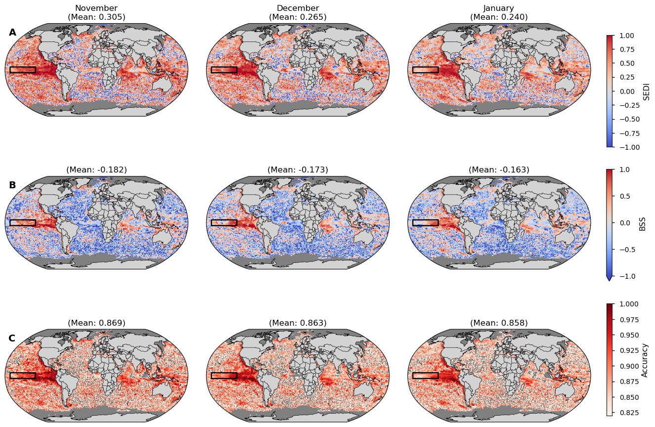
Figure 7#

Skill of Météo-France System-9 forecasts with a nominal start date October 1st for November, December, and January, using the ORAS5 reanalysis as the reference dataset. Heatwaves are defined as upper 300m ocean heat content (OHC) anomalies exceeding the 90th percentile within the 1993-2023 period. Rows show: (A) Symmetric Extremal Dependence Index (SEDI), (B) Brier Skill Score (BSS); and (C) Accuracy. In all maps, red areas indicate positive skill (forecast is better than the reference), while blue areas indicate negative skill. Masked areas are shown in grey. For the Accuracy maps (C) the areas with an accuracy lower than what would be expected by random chance (82%) are also shown with a grey color.

5. Contingency Table Analysis#

We examine the spatially-pooled contingency tables for each month to better understand the forecast behavior.

Show code cell source

Hide code cell source

def generate_contingency_tables_optimized(forecast_mask, obs_mask, normalize=False):
    """
    Generates a dictionary of contingency tables for each month.
    Uses int8.
    """
      
    # Create boolean fields. 
    obs_yes = (obs_mask == 1)
    obs_no  = (obs_mask == 0)
    fcst_yes = (forecast_mask == 1)
    fcst_no  = (forecast_mask == 0)

    # Define dimensions to sum over
    dims_to_sum = ['year', 'realization', 'latitude', 'longitude']

    TP_by_month = (obs_yes & fcst_yes).groupby('month').sum(dim=dims_to_sum)
    FN_by_month = (obs_yes & fcst_no).groupby('month').sum(dim=dims_to_sum)
    FP_by_month = (obs_no  & fcst_yes).groupby('month').sum(dim=dims_to_sum)
    TN_by_month = (obs_no  & fcst_no).groupby('month').sum(dim=dims_to_sum)

    # Execute all calculations in a single Dask operation
    #print("Computing contingency table")
    TP, FN, FP, TN = dask_compute(TP_by_month, FN_by_month, FP_by_month, TN_by_month)

    raw_tables = {}
    norm_tables = {} if normalize else None

    for month_num in TP['month'].values:
        month_name = pd.to_datetime(month_num, format='%m').month_name()
        
        tp_val = TP.sel(month=month_num).item()
        fn_val = FN.sel(month=month_num).item()
        fp_val = FP.sel(month=month_num).item()
        tn_val = TN.sel(month=month_num).item()
        
        table = pd.DataFrame(
            [[tp_val, fp_val], [fn_val, tn_val]],
            columns=['Event Observed', 'Non-event Observed'],
            index=['Event Forecasted', 'Non-event Forecasted']
        )
        
        table['Total (Forecast)'] = table.sum(axis=1)
        table.loc['Total (Observed)'] = table.sum(axis=0)
        
        raw_tables[month_name] = table.astype(int)
        
        if normalize:
            grand_total = table.loc['Total (Observed)', 'Total (Forecast)']
            if grand_total > 0:
                norm_table = (table / grand_total) * 100
                norm_tables[month_name] = norm_table
            
    if normalize:
        return raw_tables, norm_tables
    else:
        return raw_tables
        

raw_tables, percent_tables = generate_contingency_tables_optimized(
    heatwave_mask_forecast, 
    heatwave_mask_reanalysis, 
    normalize=True
)

print("\n--- Contingency Tables in Percent (%) ---")
for month_name, table in percent_tables.items():
    print(f"\n{month_name}:")
    # Format to 2 decimal places with a '%' sign
    display(table.style.format("{:.1f}%"))

--- Contingency Tables in Percent (%) ---

November:

	Event Observed	Non-event Observed	Total (Forecast)
Event Forecasted	3.2%	6.8%	10.0%
Non-event Forecasted	6.6%	83.5%	90.0%
Total (Observed)	9.7%	90.3%	100.0%

December:

	Event Observed	Non-event Observed	Total (Forecast)
Event Forecasted	2.9%	7.1%	9.9%
Non-event Forecasted	6.8%	83.2%	90.1%
Total (Observed)	9.7%	90.3%	100.0%

January:

	Event Observed	Non-event Observed	Total (Forecast)
Event Forecasted	2.6%	7.4%	10.0%
Non-event Forecasted	7.0%	83.0%	90.0%
Total (Observed)	9.6%	90.4%	100.0%

For all Novembers (one month leadtime, or 1-2 months, to be exact), when the model predicts a marine heatwave, that prediction is correct 32% of the time (Precision). Conversely, the False Discovery Rate is 68%, meaning roughly two-thirds of forecasted heatwaves did not materialize in observations. The predictive skill degrades slightly with lead time; by January (three month leadtime), the probability of a forecasted heatwave actually occurring drops to 26%.

Regarding the capture of observed events (Hit Rate), the model successfully anticipates 33% of the heatwaves that occurred in November. This capability decreases marginally to 30% in December and 27% in January. Overall, the system demonstrates an ability to capture approximately one-third of heatwave events at a one-month lead time, though users must be mindful of the high false alarm ratio.

6. Annual Variability and ENSO Influence#

We now investigate the year-to-year skill for each month and its potential connection to ENSO.

Show code cell source

Hide code cell source

def calculate_annual_skill_and_rates(forecast_mask, obs_mask):
    """
    Calculates all annual time series in a two-step process.
    Step 1: Computes float-based metrics (BSS, MHW Occ.). 
    We here use the teoretical BSSref of 0.1
    Step 2: Clears memory, then computes intiger-based metrics (SEDI, Rates)
    """
    
    fill_value = np.int8(-99)
    weights = np.cos(np.deg2rad(obs_mask.latitude))
    weights.name = "weights"

    # ---BSS in float ---
    obs_mask_float = obs_mask.where(obs_mask != fill_value).astype(np.float32)
    fcst_mask_float = forecast_mask.where(forecast_mask != fill_value).astype(np.float32)

    mhw_occurrence_lazy = obs_mask_float.weighted(weights).mean(['latitude', 'longitude']
                                                               ) * 100
    
    fct_prob = fcst_mask_float.mean('realization')
    bs_forecast = xs.brier_score(obs_mask_float, fct_prob, dim=['latitude', 'longitude'], 
                                 weights=weights)
    bs_reference_theoretical = 0.1 * (1 - 0.1)  # 0.09
    bss_theoretical_lazy = 1 - (bs_forecast / bs_reference_theoretical)

    mhw, bss = dask_compute(mhw_occurrence_lazy, bss_theoretical_lazy)

    # --- free memory ---
    del obs_mask_float, fcst_mask_float, mhw_occurrence_lazy
    del fct_prob, bs_forecast, bss_theoretical_lazy
    gc.collect();
    # -------------------

    # SEDI & Rates from the int8 arrays
    category_map = xr.where(
        obs_mask == 1,
        xr.where(forecast_mask == 1, np.int8(1), np.int8(2)),  # (TP) or (FN)
        xr.where(
            obs_mask == 0,
            xr.where(forecast_mask == 1, np.int8(3), np.int8(4)),  # (FP) or (TN)
            fill_value
        )
    ).chunk(obs_mask.chunks)

    dims_to_sum = ['realization', 'latitude', 'longitude']
    TP_ym_lazy = (category_map == 1).groupby('year').sum(dim=dims_to_sum, dtype='float32') 
    FN_ym_lazy = (category_map == 2).groupby('year').sum(dim=dims_to_sum, dtype='float32')
    FP_ym_lazy = (category_map == 3).groupby('year').sum(dim=dims_to_sum, dtype='float32')
    TN_ym_lazy = (category_map == 4).groupby('year').sum(dim=dims_to_sum, dtype='float32')

    # The int-based computations
    tp, fn, fp, tn = dask_compute(TP_ym_lazy, FN_ym_lazy, FP_ym_lazy, TN_ym_lazy)
    
    # --- free mem ---
    del category_map, TP_ym_lazy, FN_ym_lazy, FP_ym_lazy, TN_ym_lazy
    gc.collect();
    # -------------------

    # --- STEP 3: Combine results -------
    eps = 1e-12
    H = tp / (tp + fn + eps) # Hit Rate
    F = fp / (fp + tn + eps) # False Alarm Rate
    FN_rate = fn / (tp + fn + eps) # Miss Rate
    TN_rate = tn / (fp + tn + eps) # Correct Rejection Rate
    
    logH, logF = np.log(np.maximum(H, eps)), np.log(np.maximum(F, eps))
    log1mH, log1mF = np.log(np.maximum(1 - H, eps)), np.log(np.maximum(1 - F, eps))
    sedi = (logF - logH - log1mF + log1mH) / (logF + logH + log1mF + log1mH)
    
    # --- combine and format ---
    month_map = {11: 'November', 12: 'December', 1: 'January'}
    
    df_list = []
    all_metrics = {
        'MHW_Occurrence': mhw, 'BSS': bss, 'SEDI': sedi,
        'True_Pos': H, 'False_Pos': F, 'False_Neg': FN_rate, 'True_Neg': TN_rate
    }

    for name, da in all_metrics.items():
        df = da.to_dataframe(name='val').reset_index()
        df['metric'] = name + '_' + df['month'].map(month_map)
        df_list.append(df)
        
    final_df = pd.concat(df_list)
    pivot_df = final_df.pivot_table(index='year', columns='metric', values='val')
    
    return pivot_df

Annual metrics - global#

Show code cell source

Hide code cell source

roni_url = "https://www.cpc.ncep.noaa.gov/data/indices/RONI.ascii.txt"
roni_hash = "38b313ecf70be0e96967082d6a3106806fb5d8c93ae769cd819cd5276f377bac"  # se under
roni_path = pooch.retrieve(roni_url, known_hash=roni_hash)

roni_df = pd.read_csv(
    roni_path,
    sep=r"\s+",
    names=["season", "year", "anom"],
    skiprows=1,
)
roni_ndj = roni_df[roni_df["season"] == "NDJ"].set_index("year")["anom"]

# --- Plotting function ---
def plot_jacox_style_figure(df, roni_ndj, title, month_to_plot="November"):
    """
    Creates a 4-panel figure:
      Panel A (narrow): RONI NDJ bar chart (red = El Niño, blue = La Niña)
      Panel B: MHW Occurrence
      Panel C: Skill Scores (SEDI, BSS)
      Panel D: Contingency Rates

    Parameters
    ----------
    df : pd.DataFrame
        Output from calculate_annual_skill_and_rates(), indexed by year.
    roni_ndj : pd.Series
        RONI NDJ values indexed by year (from NOAA CPC RONI.ascii.txt).
    title : str
        Figure title.
    month_to_plot : str
        Which month to show in the contingency rate panel.
    """
    fig, (ax0, ax1, ax2, ax3) = plt.subplots(
        nrows=4,
        ncols=1,
        figsize=(12, 14),
        sharex=True,
        gridspec_kw={"height_ratios": [1, 2, 2, 2]},
    )
    fig.suptitle(title, fontsize=16)

    months = ["November", "December", "January"]
    styles = {"November": "-", "December": "--", "January": ":"}

    # --- Panel A: RONI NDJ index (narrow bar chart) ---
    years = df.index
    roni_vals = roni_ndj.reindex(years).values
    colors = ["#d73027" if v >= 0 else "#4575b4" for v in roni_vals]

    ax0.bar(years, roni_vals, color=colors, width=0.8, edgecolor="none")
    ax0.axhline(0.5, color="red", lw=0.6, ls="--", alpha=0.5)
    ax0.axhline(-0.5, color="blue", lw=0.6, ls="--", alpha=0.5)
    ax0.axhline(0, color="k", lw=0.5)
    ax0.set_ylabel("RONI\n(NDJ)")
    ax0.set_ylim(
        min(-2.0, np.nanmin(roni_vals) - 0.2),
        max(2.5, np.nanmax(roni_vals) + 0.2),
    )
    ax0.grid(True, linestyle=":", alpha=0.4)
    ax0.text(
        0.99, 0.95, "NCEP NOAA Relative Oceanic Niño Index",
        transform=ax0.transAxes, fontsize=8, ha="right", va="top",
        fontstyle="italic", color="0.4",
    )

    # --- Panel B: MHW Occurrence ---
    for month in months:
        ax1.plot(
            df.index, df[f"MHW_Occurrence_{month}"],
            linestyle=styles[month], label=month,
        )
    ax1.set_ylabel("MHW Occurrence (%)")
    ax1.legend(title="Month", loc="upper left")
    ax1.grid(True, linestyle=":")

    # --- Panel C: Skill Scores ---
    for month in months:
        ax2.plot(
            df.index, df[f"SEDI_{month}"],
            color="C1", linestyle=styles[month], label=f"SEDI {month}",
        )
        bss_col = (
            f"BSS_Theoretical_{month}"
            if f"BSS_Theoretical_{month}" in df.columns
            else f"BSS_{month}"
        )
        if bss_col in df.columns:
            ax2.plot(
                df.index, df[bss_col],
                color="C4", linestyle=styles[month], label=f"BSS {month}",
            )
    ax2.axhline(0, color="black", linestyle="--", linewidth=0.8)
    ax2.set_ylabel("Skill Score")
    ax2.legend(title="Metric / Month", loc="best")
    ax2.grid(True, linestyle=":")

    # --- Panel D: Contingency Rates ---
    ax3.plot(
        df.index, df[f"True_Pos_{month_to_plot}"],
        color="C0", label="True Pos. (Hit Rate)",
    )
    ax3.plot(
        df.index, df[f"True_Neg_{month_to_plot}"],
        color="C3", label="True Neg. Rate",
    )
    ax3.plot(
        df.index, df[f"False_Pos_{month_to_plot}"],
        color="C2", label="False Pos. (False Alarm Rate)",
    )
    ax3.plot(
        df.index, df[f"False_Neg_{month_to_plot}"],
        color="C5", label="False Neg. (Miss Rate)",
    )
    ax3.set_ylabel("Rate")
    ax3.set_xlabel("Year")
    ax3.legend(title=f"Rates for {month_to_plot}", loc="best")
    ax3.grid(True, linestyle=":")

    # Shared x-axis limits
    for ax in [ax0, ax1, ax2, ax3]:
        ax.set_xlim(df.index.min() - 1, df.index.max() + 1)

    plt.tight_layout(rect=[0, 0.03, 1, 0.95])
    plt.show()

    # 2. Run global calculation and plot
global_jacox_df = calculate_annual_skill_and_rates(
    heatwave_mask_forecast, 
    heatwave_mask_reanalysis
)

plot_jacox_style_figure(
    global_jacox_df, 
    roni_ndj,
    title="Annual Forecast Skill for NDJ Heatwaves (Global Average)"
)

../_images/539a4c12985bfc453099088956943d770020db0444d314a1a871414f3d7c55ed.png

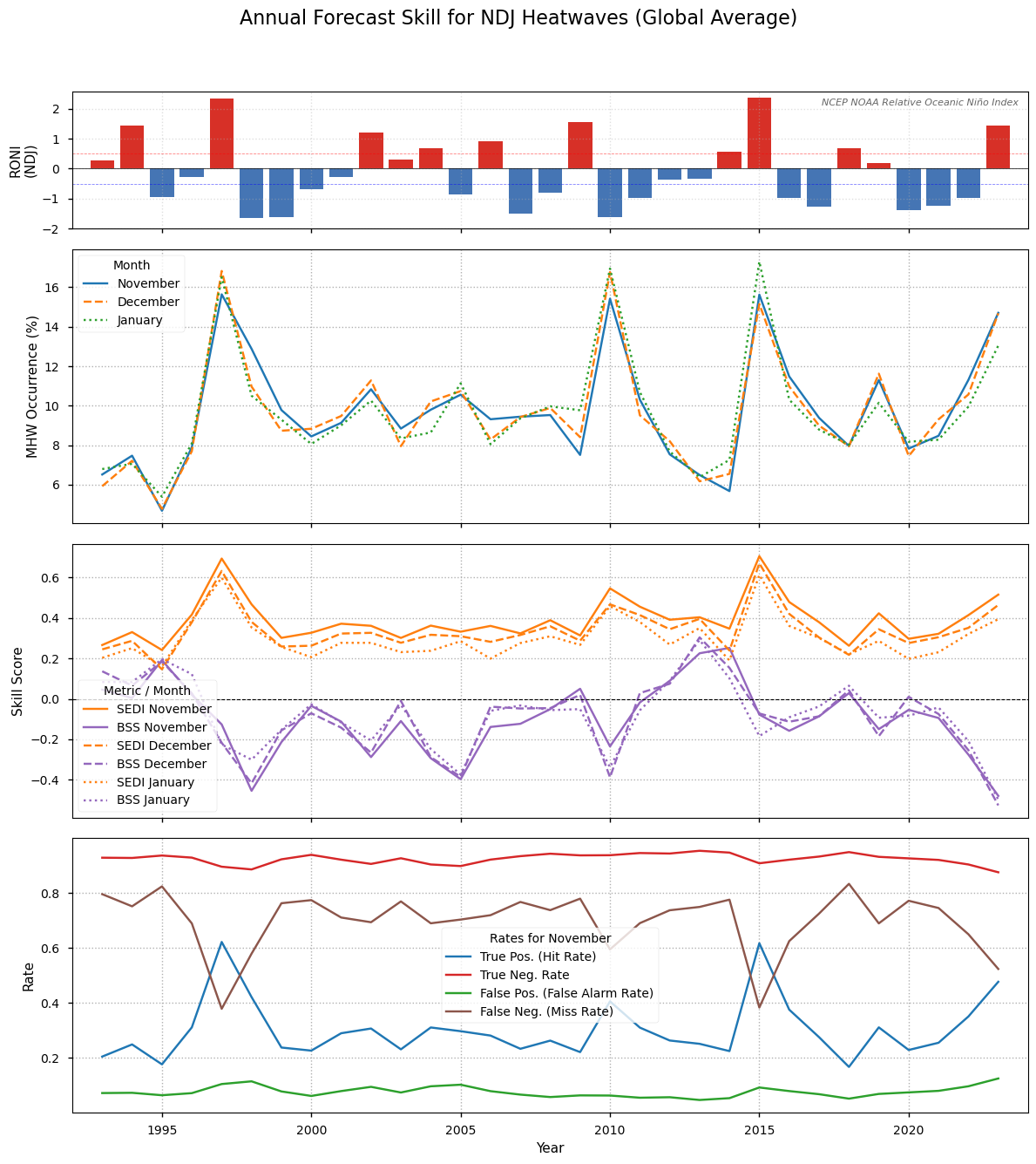
Figure 8#

Annual time series of globally-averaged forecast performance for the NDJ season. The upper panel depticts occurrence of El Niño according to the NCEP NOAA Relative Oceanic Niño Index (RONI), defines as the three month running average of the relative Niño 3.4 index. The second row depicts global marine heatwave (MHW) occurrence each year, i.e. the percentage of gridcells in heatwave conditions. The third plot shows the SEDI and the BSS in NDJ averaged over the valid ocean region. The contingency table components, the False or True Positives and Negatives each year for a selected month, November, are shown in the lower plot. The figure is similar to Extended Data Fig. 5 in Jacox et. al. 2022, [1].

An analysis of global year-to-year variability in SEDI and BSS (Figure 8) reveals a divergence in skill metrics. The SEDI scores (orange lines) remain positive and notably peak during major El Niño events (e.g., 1997-98, 2015-16). This indicates that the forecast system is highly effective at signal detection; it successfully identifies high-risk periods during these major climate drivers. Conversely, the BSS (purple lines), which measures probabilistic skill, often deteriorates during these same events. This might indicate that the single-model system is overconfident. The distribution analysis (Figure 4) shows that the reference reanalysis exhibits a sharper tail than the forecast ensemble. While the model often captures the correct warming signal, this lower extreme-tail variability may be linked to the observed overconfidence in its probabilistic assignments.

While the model correctly predicts the risk of a heatwave (high SEDI), the probability it assigns is less accurate. This is a common limitation of single-model systems, where the ensemble spread is insufficient to represent true uncertainty. Transitioning to a multi-model ensemble would likely improve reliability for decision-making by increasing that spread.

We focus on a key area: the Niño 3.4 region (5°N-5°S, 170-120°W). The Niño 3.4 region was chosen as it represents the tropical pacific and the ENSO.

Annual metrics - Niño 3.4 region#

--- Running Case Study: Niño 3.4 Region ---

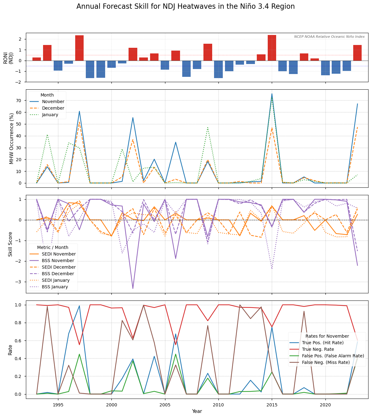
../_images/351e9709f879080771a3a80127e2582021e77b283b5ea9fd9a566a8f0e6fbfa2.png

Figure 9#

As in Figure 8, but for the Niño 3.4 region.

In contrast, the skill within the Niño 3.4 region (Figure 9) is much higher and more reliable. Although the time-series exhibits higher variability, which is expected a dynamic and smaller region, the BSS is consistently positive, approaching 1.0 during the major 1997-98 and 2015-16 events. The high SEDI scores further confirm the model’s ability to capture these extremes. This confirms that the probabilistic forecasts are both skillful and reliable regarding marine heatwaves during ENSO events, which are the primary driver of seasonal predictability.

Summary of Results#

This study compares the Météo-France System-9 seasonal forecasts against the ORAS5 ocean reanalysis for forecasts initialized around October 1st for mean monthly values in November, December, and January. The analysis focused on the forecast skill for extreme upper OHC events (anomalies >90th percentile) after removing long-term trends from both datasets. By looking at anomalies, detrending the data, and applying lead-time (or calendar month) dependent percentiles we do our best to match the seasonal data with the reference data. We assess skill 1–3 months after the forecasts nominal start date using metrics such as the Symmetric Extremal Dependence Index (SEDI) and the Brier Skill Score (BSS). The metrics considered follow Jacox et al. (2022) [1], however, in this work we look at OHC and not SST. It should be noted that this evaluation and use-case considers a single ocean reanalysis as a reference dataset. Using an ensemble of observational datasets could provide a more robust assessment.

The forecast system demonstrates clear, positive skill in detecting events. The Symmetric Extremal Dependence Index (SEDI) is positive globally and spikes during major El Niño events (e.g., 1997-98, 2015-16). This is corroborated by the contingency rate analysis (Figure 8 lower panel), which shows the True Positive (Hit) Rate increasing dramatically in these years, confirming the model successfully captures the El Niño signal, and the corresponding effect on the MHW index derived from the ocean heat content.

The system provides a valuable tool for anticipation of NDJ upper ocean heatwaves, with its utility and reliability being highest in ENSO-dominated regions. However, outside this region the Brier Skill Score (BSS) is often negative, indicating that the forecast probabilities are less reliable than the static climatological reference forecast (always a 10% chance). This might indicate that the model has too little ensemble spread in these regions. This makes the forecast a good “heads-up” warning for high-risk periods, but for higher reliability outside the main ENSO regions a multi-model system might be useful.

ℹ️ If you want to know more#

Key resources#

Seasonal forecast monthly averages of ocean variables DOI: 10.24381/cds.2f9be611

ORAS5 global ocean reanalysis monthly data from 1958 to present DOI: 10.24381/cds.67e8eeb7

Code libraries used:

C3S EQC custom functions, c3s_eqc_automatic_quality_control, prepared and advised on by B-Open
xesmf
ocean-regrid make_corners to provide cell edge coordinates for the ORCA025 tripolar grid
xskillscore
dask
xarray
pandas
matplotlib
seaborn
scipy
numpy
cartopy

References#

[1] Jacox, M. G., Alexander, M. A., Amaya, D., Becker, E., Bograd, S. J., Brodie, S., Hazen, E. L., Pozo Buil, M., & Tommasi, D. (2022). Global seasonal forecasts of marine heatwaves. Nature, 604(7906), 486–490.

[2] McAdam, R., Masina, S., Balmaseda, M., Gualdi, S., Senan, R., & Mayer, M. (2022). Seasonal forecast skill of upper-ocean heat content in coupled high-resolution systems. Climate Dynamics, 58(11–12), 3335–3350.

[3] Specq, D., Dorel, L., Beuvier, J., Ardilouze, C., & Batté, L. (2024). Documentation of the Météo-France seasonal forecasting system 9. Zenodo.

[4] Ferro, C. A. T., & Stephenson, D. B. (2011). Extremal Dependence Indices: Improved Verification Measures for Deterministic Forecasts of Rare Binary Events. Weather and Forecasting, 26(5), 699–713.

Seasonal Forecast Prediction of Upper Ocean Heat Content Extremes

Contents

4.1. Seasonal Forecast Prediction of Upper Ocean Heat Content Extremes#

🌍 Use case: Predicting upper ocean heat content extremes in climate services#

❓ Quality assessment question#

📢 Quality assessment statement#

📋 Methodology#

Pooling and grouping strategies#

SEDI - the Symmetric Extremal Dependence Index#

The Brier Skill Score (BSS)#

Accuracy#

📈 Analysis and results#

1. Data Preparation#

Imports and Settings#

Definition of Parameters#

Helper Functions for Data Processing and Plotting#

Data Loading#

2. OHC Time Series and Trend Analysis#

Figure 2#

3. Model Performance vs. Reanalysis#

Correlation of OHC Anomalies#

Figure 3#

Comparison of distributions#

Figure 4#

Comparison of Heatwave Representation#

Figure 5#

Diagnostic Plots.#

Figure 6#

4. Metrics: SEDI, BSS, Accuracy#

Symmetric Extremal Dependence Index (SEDI)#

The Brier Skill Score (BSS)#

Accuracy Assessment#

Pooling Strategy for Skill Metrics in Map Form#

Findings#

Figure 7#

5. Contingency Table Analysis#

6. Annual Variability and ENSO Influence#

Annual metrics - global#

Figure 8#

Annual metrics - Niño 3.4 region#

Figure 9#

Summary of Results#

ℹ️ If you want to know more#

Key resources#

References#