

1.2.3. Spatial resolution and completeness of carbon dioxide satellite observations for quantifying carbon fluxes#
Production date: 09-04-2026
Produced by: Paolo Cristofanelli (CNR)
Note
Please note that this assessment also refers to the deprecated Level 2 XCO\(_2\) data products which won’t be extended after 2022.
🌍 Use case: Using satellite observations for investigating the global carbon fluxes#
❓ Quality assessment question#
Are the CO\(_2\) satellite observations suitable for deriving global and regional carbon fluxes in terms of resolution and spatial completeness?
Carbon dioxide (CO\(_2\)) is the most important anthropogenic greenhouse gas, accounting for almost 64% of the total radiative forcing by long-lived greenhouse gases [1]. The atmospheric concentration of CO\(_2\) in 2023 was 419.3\(\,\pm\,\)0.1 ppm [2].
Accurate spatial and temporal quantification of carbon dioxide (CO\(_2\)) is central to understanding the carbon cycle and supporting policy decisions on climate change mitigation. Satellite retrievals (Level 2 data products) of column-averaged dry air mole fractions of CO\(_2\) (XCO\(_2\)) have been widely used to infer regional and global variations in carbon fluxes through atmospheric inversion modelling (e.g., [3], [4], [5], [6], [7], [8]).
Atmospheric inverse modelling [9] links CO\(_2\) fluxes to observed atmospheric CO\(_2\) mole fractions (like those provided by satellite measurements) using atmospheric transport (and chemistry) models, and is often referred to as “top-down” approach. Typically “top-down” inverse systems estimate residual natural or fluxes not related to fossil fuel consumption and cement production (FFC) from land and ocean regions (e.g., [10] and [7]).
Atmospheric inversion systems estimate carbon fluxes by adjusting modelled CO\(_2\) fluxes to match atmospheric observations. The so-called “a‑priori” flux fields provide initial modelled CO\(_2\) fluxes by combining, e.g., estimates of anthropogenic emissions from statistical inventories, terrestrial biosphere and oceanic fluxes from models or climatologies and emissions from vegetation fires. An example of a global-scale inversion system and adopted “a-priori” fields is represented by the CAMS “PYVAR” inversion system [11].
Due to their large spatial coverage, satellite observations are used for constraining atmospheric inversions by complementing independent datasets provided by high-precision in-situ measurements like those provided by [12].
In this assessment, through a review of existing literature and use cases combined with specific data analyses, we investigate if the spatial resolution and coverage of the dataset “Carbon dioxide data from 2002 to present derived from satellite observations” provided by [13] are suitable to constrain global and regional Earth’s carbon fluxes in “top-down” inversion systems.
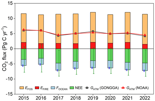
The figure shows the global carbon budget estimated by the Global ObservatioN-based system for monitoring Greenhouse GAses (GONGGA) atmospheric inversion system through assimilation of Orbiting Carbon Observatory-2 (OCO-2) XCO\(_2\) data and the global atmospheric growth rate by [12]. \(E_{\mathrm{FOS}}\) denotes fossil fuel CO\(_2\) emissions, \(E_{\mathrm{FIRE}}\) denotes biomass combustion emissions, \(F_{\mathrm{OCEAN}}\) denotes ocean-atmosphere carbon fluxes, NEE denotes net ecosystem exchange (i.e. the balance of photosynthesis and respiration from the terrestrial ecosystem) and \(G_{\mathrm{ATM}}\)denotes the growth rate of atmospheric CO\(_2\) concentration derived from GONGGA and [12]. Image reproduced from [7] under CC-BY licence.
📢 Quality assessment statement#
These are the key outcomes of this assessment
The XCO2_OBS4MIPS Level 3 product has been primarily generated for comparison with climate models and has also been used for computations of annual mean atmospheric growth rates. This data product in not recommended to derive global and regional carbon fluxes.
In terms of spatial resolution, the mid-tropospheric-averaged air mole fractions of CO\(_2\) (MTCO2_OBS4MIPS, Level 3) data product appears appropriate for use in global and regional inversion system. However, users must carefully consider limitations related with spatial completeness (mostly limited to tropical regions) and vertical representativeness. As there are no known applications of this MT-CO\(_2\) product, extreme caution should be exercised to use this data product to derive global and regional carbon fluxes by inversion modelling systems.
The deprecated Level 2 XCO\(_2\) datasets can be used within inversion modelling systems to derive historical global and regional carbon fluxes. Users would use the data product derived by the algorithm XCO2_EMMA that optimise data availability over regions frequently affected by cloud cover or high aerosol loading.
The spatial coverage and resolution (spatial density) of the satellite data or a combination of them, affected the impact of satellite observations on carbon flux quantifications in different regions.
As the MTCO2_OBS4MIPS dataset is updated every six months and Level 2 XCO\(_2\) won’t be extended in time after 2022, users interested in more timely greenhouse gas fluxes quantification should consider other Copernicus resources.
📋 Methodology#
To evaluate if the spatial coverage and resolution of satellite-based observations characterizing the Climate Data Store dataset “Carbon dioxide data from 2002 to present derived from satellite observations” [13] are suitable for their usage in an atmospheric inversion system to investigate Earth’s carbon fluxes, we inspected the related CDS Documentation [14] as well as external references like [15], and case studies available from scientific literature ([3], [5], [6], [7]) and applications (e.g., [8], [11]). Moreover, we performed specific analyses on the spatial data coverage of the Level 3 data product Obs4MIPs (version 4.6) and IASI-MERGED-OBS4MIPS (version 10.1).
In particular:
[3] inferred regional estimates of the European land carbon sink by performing a regional surface flux inversion using earlier versions of the XCO\(_2\) satellite measurements from SCIAMACHY (BESD v02.00.08 and) and GOSAT (ACOS v3.4r03 2010, UoLFP v4.0 2010, RemoTeC v2.11 2010, and NIES v02.xx 2010) than those available from the Climate Data Store dataset “Carbon dioxide data from 2002 to present derived from satellite observations” [13].
[5] evaluated an ensemble of six multi-year global CO\(_2\) atmospheric inversions by using a large dataset of accurate aircraft measurements in the free troposphere over the globe. For the inversion experiments, besides using OCO-2 data (ACOS bias-corrected retrievals, version 9), they also considered a previous version of a Level 2 data product available by the Climate Data Store (CO2_GOS_OCFP, v7.1).
[6] compared the results of constraining the terrestrial ecosystem carbon fluxes by assimilating GOSAT and OCO-2 XCO\(_2\) retrievals (both produced by the “NASA Atmospheric CO\(_2\) Observations from Space” project, version b7.3) within the GEOS-Chem 4D-Var assimilation framework.
[7] presented a global spatially resolved terrestrial and ocean carbon flux dataset for years 2015–2022 generated by an atmospheric inversion system through the assimilation of OCO-2 XCO\(_2\) retrievals (Level 2, Lite v11r data product).
[8] provide a case about the use of CO\(_2\) satellite observations to estimate net CO\(_2\) fluxes into the atmosphere at global scale and over specific land and oceans regions by using the CAMS global inversion systems. This inversion system uses in-situ atmospheric observations from large living databases, like NOAA Earth System Research Laboratory Observation Package, Integrated Carbon Observation System, and satellite retrievals from OCO-2.
Please note that the analysed references referred to the use of Level 2 data products within atmospheric inversion systems, for which there are example applications. Level 3 data products for satellite XCO\(_2\) or MT-CO\(_2\) have not yet been used in inversion systems to derive quantifications of surface CO\(_2\) fluxes. However, a critical comparison of the resolution and completeness features of the Level 3 data products with respect to known applications based on Level 2 data products has been performed.
In the following, we report the outline of this notebook.
1. Set-up the code and choose the data to use
Import all relevant packages.
Cache needed functions.
Define the data request to CDS.
3. Spatial resolution assessment
We compared the spatial resolution of the “Carbon dioxide data from 2002 to present derived from satellite observations” [13] data products with those of the the satellite datasets used by atmospheric inversion experiments documented above.
4. Spatial completeness assessment
We created plots of the monthly mean data coverage of the Level 3 data product Obs4MIPs (version 4.6) and IASI-MERGED-OBS4MIPS (version 10.1) and we compared them with those of the satellite datasets used by atmospheric inversion experiments documented above. Moreover, we also considered external documentation ([15]) to assess the spatial coverage of the (deprecated) Level 2 data products part of the “Carbon dioxide data from 2002 to present derived from satellite observations” [13] dataset.
5. How suitable are these datasets for ingestion into inversion systems?
We provide a summary of the main outcomes of this assessment.
📈 Analysis and results#
1. Set-up the code and choose the data to use#
Import all relevant packages#
In this section, we import all the relevant packages needed for running the notebook.
Cache needed functions#
In this section, we cached a list of functions used in the analyses.
The
convert_unitsfunction rescales XCO\(_2\) mole fraction to parts per million (ppm).The
compute_coverage_obs4mipsfunction calculates the spatial fractional coverage of the available data for the Obs4MIPs Level 3 dataset.The
compute_coverage_iasiandaggregate_coverage_iasifunctions calculate the spatial fractional coverage of the available data for the IASI-MERGED-OBS4MIPS Level 3 dataset.
2. Retrieve data#
2.1 Obs4MIPs#
In this section, we define the data request to CDS (data product Obs4MIPs, Level 3, version 4.6, XCO\(_2\)) and download the full dataset.
2.2 IASI-MERGED-OBS4MIPS#
In this section, we define the data request to CDS (data product IASI-MERGED-OBS4MIPS, Level 3, version 10.1, MT-CO\(_2\)) and download the full dataset (please note that users can modify the time period).
3. Spatial resolution assessment#
Ideally, the spatial resolution of the satellite observations used in an inversion system should match that of the transport model. In turn, the transport model should match the spatial scale of carbon fluxes, which is typically on the order of hundreds of metres. In practice, however, contemporary models generally have much coarser resolutions, typically on the order of degrees ([16]), and errors in the simulated atmospheric transport may also affect the inversion results ([17]).
The documented use cases ([5], [6],[7], [8]) used OCO-2 observations characterised by spatially dense data with a narrow swath (10.3 km) and with footprints of a few square kilometres (1.29 km × 2.25 km). [5] and [6] also used a previous version of the CDS GOSAT Level 2 deprecated dataset, characterised by a coarser-resolution data (100 km\(^2\) at nadir) with lower spatial density than OCO-2. A more recent application is the inversion system that generates the CAMS global CO\(_2\) atmospheric inversion product (PyVAR, see [11]): it uses OCO-2 bias-corrected land retrievals of XCO\(_2\) after averaging glint and nadir OCO-2 retrievals in 10-s bins (corresponding to a ground-track swaths of 67 km) to match the transport model horizontal spatial resolution of about 90 km\(^{2}\).
XCO2_OBS4MIPS Level 3: the spatial aggregation at 5° × 5° resolution and the temporal aggregation at monthly scales inevitably reduce the amount of information available to the inversion system. Such levels of aggregation are not commonly adopted in global or regional inverse modeling studies (see, e.g., [5], [6], [11]): indeed, this data product has primarily been generated for comparison with climate models and climate monitoring, rather than for the quantification of carbon fluxes through the ingestion-inversion system.
MTCO2_OBS4MIPS Level 3 : this dataset is new and thus never used before. However, Level 2 MT-CO2 and MT-CH4 products have been used for flux inversions ([18], [19]) and the current spatial (1° x 1°) and temporal (1 day) resolution of this Level 3 data product can potentially meet the requirements for the investigation of carbon fluxes at regional and global scales (see, e.g. [11]).
Level 2 (deprecated): GOSAT and GOSAT-2 measurements (CO2_GOS_SRFP v2.3.8, CO2_GOS_OCFP v7.3, CO2_GO2_SRFP v2.1.0) are characterised by a 9.7 km (diameter) footprint with the single observations typically on the order of 100 km apart with a 6-day repeat cycle. [5] and [6] used previous versions of the GOSAT Level 2 deprecated dataset. According to [5], the lower data density of GOSAT observations with respect to OCO-2 may potentially affect the quantification of carbon fluxes but no conclusive statements were made on this topic. For use with an inverse modelling system, interested users may also consider the deprecated Level 2 merged multi-sensor XCO2_EMMA data product that consists of individual Level 2 soundings retrieved by different sensors (including also OCO-2) and algorithms ([20]).
4. Spatial completeness assessment#
The impact of satellite data on the carbon fluxes diagnosed by the inversion system is affected by to the spatial coverage and by the amount of data provided by the satellite measurements. In general, for regions characterised by low data coverage, the carbon fluxes diagnosed by the inversion system are dominated by the information provided by the “a-priori” fields (see [6]). As documented by [5] and [6], both OCO-2 and GOSAT observations are not evenly distributed spatially.
Due to cloud contamination, there are few retrievals in a large portion of tropical land. When clouds are present, they act as opaque or semi-opaque barriers to the solar radiation reflected at the Earth’s surface, meaning that the radiation reflected from the cloud top does not carry information about the gases below the clouds.
Moreover, available satellite retrievals are very sparse in the northern high-latitude area, especially in boreal regions, due to the occurrence of low solar zenith angles (SZAs). This is because high SZAs, which are typical of regions at high latitudes, complicate retrievals due to weaker illumination. This reduces the satellite radiance signal, making retrievals noisier and more uncertain. Furthermore, the long slant paths under high SZAs amplify the influence of aerosol scattering and cirrus clouds, which can result in errors in the retrieved gas amount. Furthermore, they cause multiple scattering and path-length uncertainty, which can affect satellite radiance observations in the near infrared/short wave infrared (NIR/SWIR) spectral region. As reported by [21], the specific retrieval difficulties depend on the retrieval algorithm adopted.
XCO2_OBS4MIPS Level 3: this is a global dataset, obtained by gridding the merged Level 2 products generated with the ensemble median algorithm (XCO2_EMMA, see [21]). EMMA combines several different XCO\(_2\) level-2 satellite data products: SCIAMACHY/Envisat (2003–2012), TANSO-FTS/GOSAT (2009–2022), OCO-2 (2014-2022), TANSO-FTS-2/GOSAT2 (2019-2023). The completeness of the spatial data varies with the seasons due to the above-described limitations in retrieving XCO\(_2\) (i.e. low reflected sunlight during periods characterised by low SZAs, and surface shielding due to clouds). Data for the Southern Hemisphere (SH) mid and high latitudes is available from September to March, whereas data for the Northern Hemisphere (NH) mid and high latitudes is mostly available from April to August. Furthermore, the number of available observations depends significantly on location, with low coverage over areas typically affected by high cloud (such as the tropics).
100%|██████████| 1/1 [00:00<00:00, 1.95it/s]
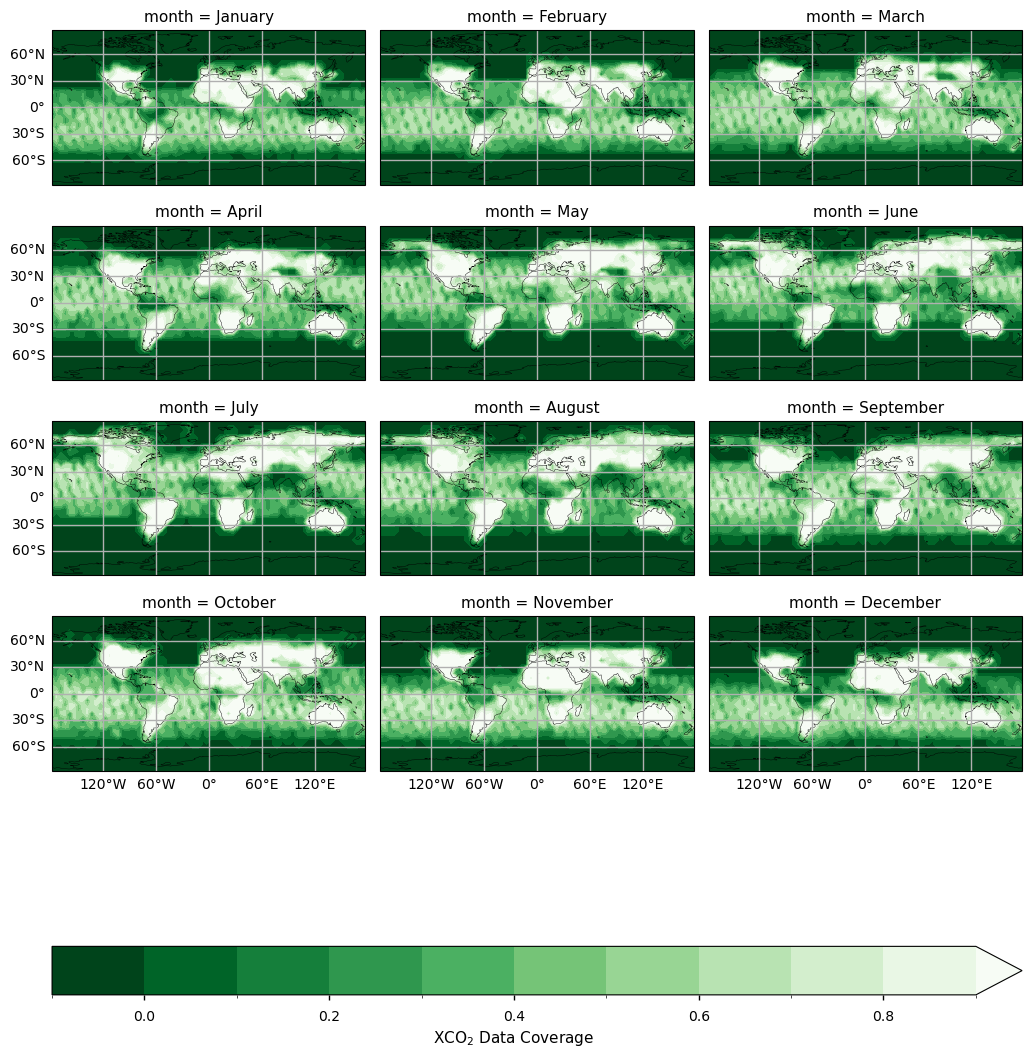
The figure shows the monthly fractional XCO\(_2\) data coverage from 2003 to 2023 derived from the XCO2_OBS4MIPS dataset (version 4.6). Please note that the colour scale has been set to optimise visualisation of the spatial path of the data coverage.
MTCO2_OBS4MIPS Level 3: as described in the Documentation [22], the dataset is mostly limited to tropical air masses (between about 30°N and 30°S) due to the fact that decorrelation between CO\(_2\) and temperature signals in the IASI radiances is more complex outside of the tropical region, yielding too high retrieval uncertainty. Moreover, it should be stressed that this is a mid‑troposphere product with the highest sensitivity of the measurements around 250 hPa (see [28]), while surface CO\(_2\) fluxes imprint their strongest signals in the boundary layer (0–2 km). This implies potential limitations in the ability of this dataset in constraining surface CO\(_2\) fluxes.
100%|██████████| 210/210 [01:31<00:00, 2.30it/s]
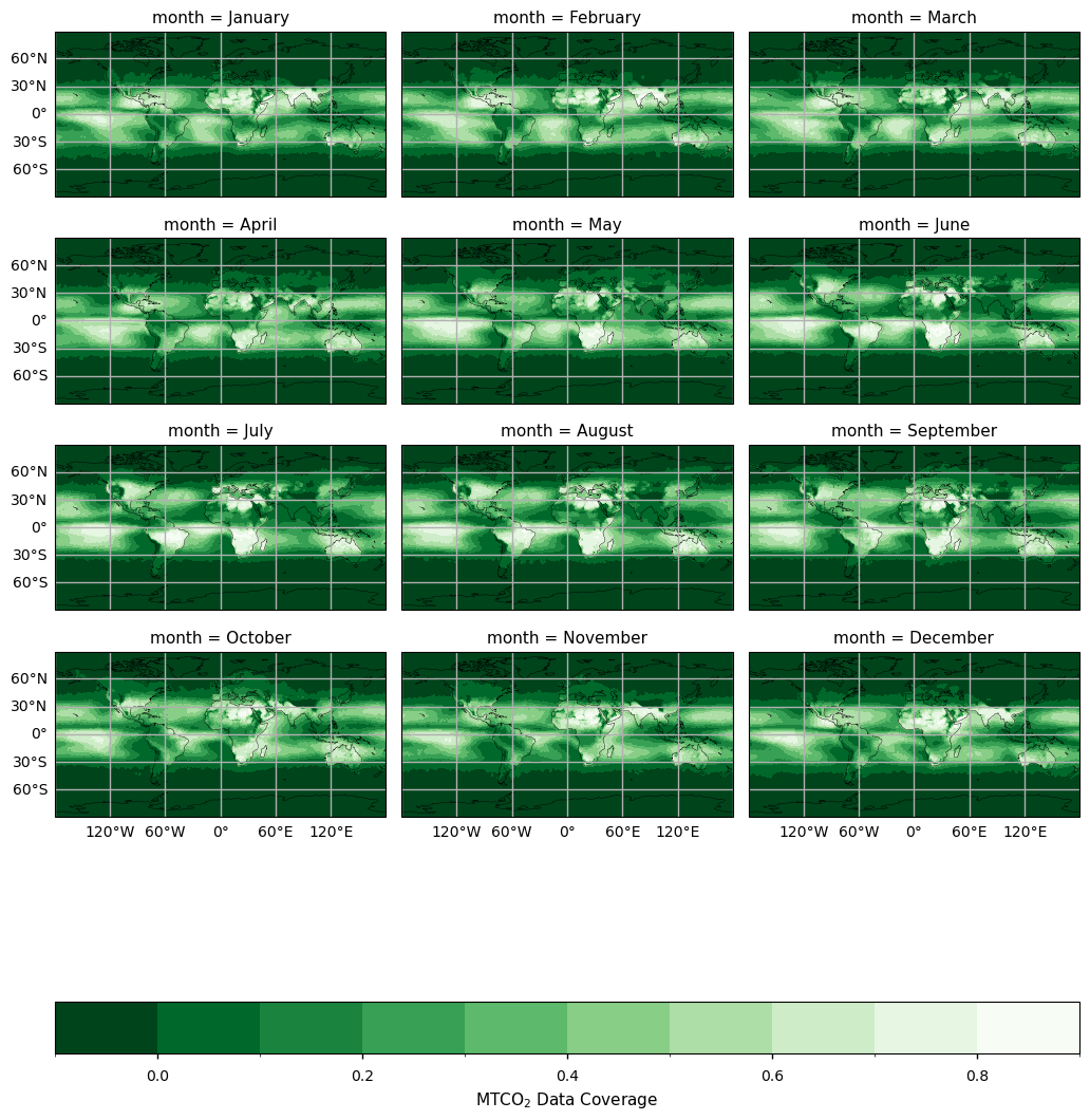
The figure shows the monthly fractional XCO\(_2\) data coverage from 2007 to 2024 derived from the IASI-MERGED-OBS4MIPS (version 10.1). Please note that the colour scale has been set to optimise visualisation of the spatial path of the data coverage.
Level 2 (deprecated): with respect to spatial completeness GOSAT data products are characterised by low data coverage at high latitudes (due to unfavourable illumination conditions) and over the tropics (due to frequent cloud contamination). For use with an inverse modelling system to obtain information on CO\(_2\) surface fluxes, interested users may also consider the Level 2 merged multi-sensor XCO2_EMMA data product ([20]) that optimises the spatial and the temporal data coverage by merging XCO\(_2\) data from different sensors and algorithms. The XCO2_EMMA data product consists of individual Level 2 soundings retrieved by algorithms that may vary from gridbox to gridbox and from month to month. As recommended by [23], it is important to note that these merged products are not necessarily the most optimal products for all applications, as they do not include all data from a given satellite sensor.
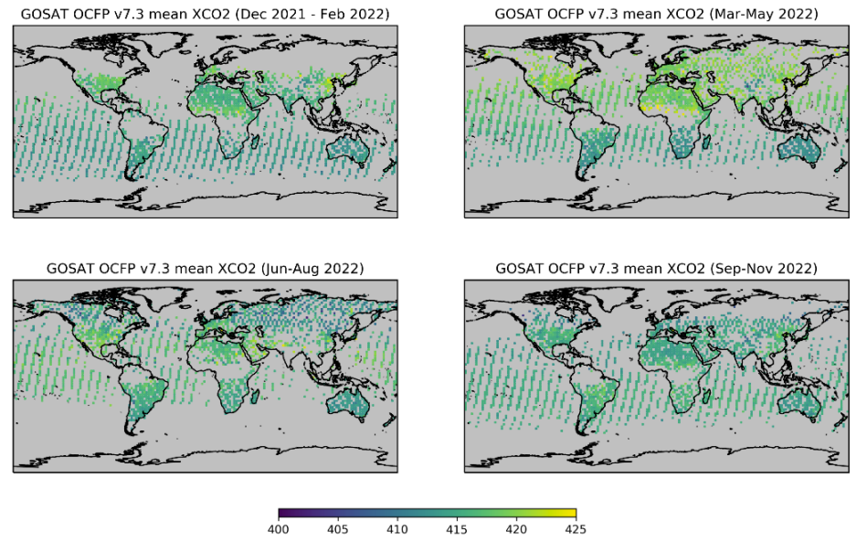
Figure showing global seasonal maps of GOSAT XCO2 “CO2_GOS_OCFP” retrieved between December 2021 and November 2022. XCO\(_2\) values are expresssed as parts per million (ppm). Image adapted from [24] under CC-BY license.
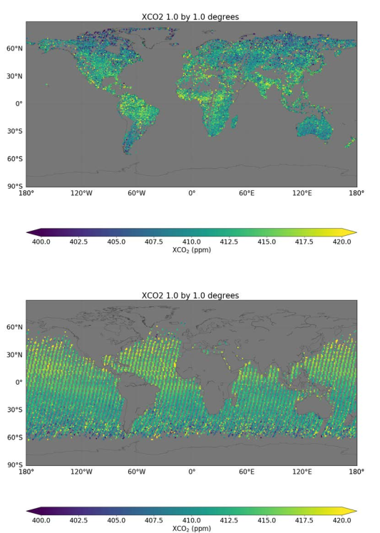
Figure showing global XCO\(_2\) map of GOSAT XCO2 “CO2_GO2_SRFP” for the 2019-2022 period on a 1° X 1° resolution for both land (top) and ocean (bottom) retrievals. XCO\(_2\) values are expresssed as parts per million (ppm). Image adapted from [25] under CC-BY license.
5. How suitable are these datasets for ingestion into inversion systems?#
In this section, we summarise the features of the “Carbon dioxide data from 2002 to present derived from satellite observations” dataset (13) in terms of spatial resolution and completeness, in order to constrain the “top-down” inversion systems of global and regional Earth’s carbon fluxes. Please note that Level 3 XCO\(_2\) or MT-CO\(_2\) satellite data products have not yet been used in inversion systems to derive surface CO\(_2\) flux quantifications. Thus, the outcomes of this assessment, especially for the MT-CO2_OBS4MIPS data product, may change in the future if applications become available.
XCO2_OBS4MIPS Level 3: This data product is characterised by temporal (monthly) and spatial (5° x 5°) resolutions higher that those typically used to quantify surface CO\(_2\) fluxes by inversion systems. Also considering that no applications currently exist for using this XCO\(_2\) data product, it cannot be recommended for quantifying surface CO\(_2\) fluxes by inversion modelling systems.
MTCO2_OBS4MIPS Level 3: This data product is characterised by temporal (daily) and spatial (1° x 1°) resolutions consistent with those reported in the scientific literature and use cases for use in an inversion system. The data product is primarily limited to tropical air masses (between approximately 30°N and 30°S), with the highest measurement sensitivity around 250 hPa. This implies potential limitations for this data product to constrain surface CO\(_2\) fluxes. As there are currently no applications for using this MT-CO\(_2\) data product, extreme caution should be exercised when using it to quantify surface CO\(_2\) fluxes through inversion modelling systems.
Level 2 (deprecated): these XCO\(_2\) data products are suitable to be ingested in inversion modelling systems for the quantification of historical (2002 - 2022) surface CO\(_2\) fluxes. In particular, users may consider the XCO2_EMMA data product that optimises the spatial and the temporal data coverage.
Note
Please note that this assessment was not produced to rank the distinctive performance of the OCO-2 and GOSAT datasets in atmospheric inversion systems. Differences in the results of inversion experiments can be related to different factors, some of which are related to the satellite observations used (such as their data coverage, data precision, data accuracy including the implemented bias correction), while others can be related to other components of the inversion system (e.g. the transport model used, the “a-priori” field, the inversion method used).
ℹ️ If you want to know more#
Key resources#
The CDS catalogue entries for the data used were:
Carbon dioxide data from 2002 to present derived from satellite observations: https://cds.climate.copernicus.eu/datasets/satellite-carbon-dioxide?tab=overview
Users interested in accessing CO\(_2\) fluxes from inversion systems can consider to use specifically designed Copernicus resources like CAMS global inversion-optimised greenhouse gas fluxes and concentrations.
References#
[1] World Meteorological Organization. (2023). WMO Greenhouse Gas Bulletin, 19, ISSN 2078-0796.
[2] Friedlingstein, P., O’Sullivan, M., Jones, M. W., Andrew, R. M., Hauck, J., Landschützer, P., Le Quéré, C., Li, H., Luijkx, I. T., Olsen, A., Peters, G. P., Peters, W., Pongratz, J., Schwingshackl, C., Sitch, S., Canadell, J. G., Ciais, P., Jackson, R. B., Alin, S. R., Arneth, A., Arora, V., Bates, N. R., Becker, M., Bellouin, N., Berghoff, C. F., Bittig, H. C., Bopp, L., Cadule, P., Campbell, K., Chamberlain, M. A., Chandra, N., Chevallier, F., Chini, L. P., Colligan, T., Decayeux, J., Djeutchouang, L. M., Dou, X., Duran Rojas, C., Enyo, K., Evans, W., Fay, A. R., Feely, R. A., Ford, D. J., Foster, A., Gasser, T., Gehlen, M., Gkritzalis, T., Grassi, G., Gregor, L., Gruber, N., Gürses, Ö., Harris, I., Hefner, M., Heinke, J., Hurtt, G. C., Iida, Y., Ilyina, T., Jacobson, A. R., Jain, A. K., Jarníková, T., Jersild, A., Jiang, F., Jin, Z., Kato, E., Keeling, R. F., Klein Goldewijk, K., Knauer, J., Korsbakken, J. I., Lan, X., Lauvset, S. K., Lefèvre, N., Liu, Z., Liu, J., Ma, L., Maksyutov, S., Marland, G., Mayot, N., McGuire, P. C., Metzl, N., Monacci, N. M., Morgan, E. J., Nakaoka, S.-I., Neill, C., Niwa, Y., Nützel, T., Olivier, L., Ono, T., Palmer, P. I., Pierrot, D., Qin, Z., Resplandy, L., Roobaert, A., Rosan, T. M., Rödenbeck, C., Schwinger, J., Smallman, T. L., Smith, S. M., Sospedra-Alfonso, R., Steinhoff, T., Sun, Q., Sutton, A. J., Séférian, R., Takao, S., Tatebe, H., Tian, H., Tilbrook, B., Torres, O., Tourigny, E., Tsujino, H., Tubiello, F., van der Werf, G., Wanninkhof, R., Wang, X., Yang, D., Yang, X., Yu, Z., Yuan, W., Yue, X., Zaehle, S., Zeng, N., and Zeng, J. (2025). Global Carbon Budget 2024, Earth System Science Data, 17, 965-1039. https://doi.org/10.5194/essd-17-965-2025
[3] Reuter, M., Buchwitz, M., Hilker, M., Heymann, J., Schneising, O., Pillai, D., Bovensmann, H., Burrows, J. P., Bösch, H., Parker, R., Butz, A., Hasekamp, O., O’Dell, C. W., Yoshida, Y., Gerbig, C., Nehrkorn, T., Deutscher, N. M., Warneke, T., Notholt, J., Hase, F., Kivi, R., Sussmann, R., Machida, T., Matsueda, H., and Sawa, Y. (2013). Satellite-inferred European carbon sink larger than expected. Atmospheric Chemistry and Physics, 14, 13739–13753. https://doi.org/10.5194/acp-14-13739-2014
[4] Reuter, M., and Coauthors. (2017). How much CO\(_2\) is taken up by the European terrestrial biosphere?. Bullettin of American Meteorology Society, 98, 665–671. https://doi.org/10.1175/BAMS-D-15-00310.1
[5] Chevallier, F., Remaud, M., O’Dell, C. W., Baker, D., Peylin, P., and Cozic, A. (2019). Objective evaluation of surface- and satellite-driven carbon dioxide atmospheric inversions. Atmospheric Chemistry and Physics, 19, 14233–14251. https://doi.org/10.5194/acp-19-14233-2019
[6] Wang, H., Jiang, F., Wang, J., Ju, W., and Chen, J. M. (2019). Terrestrial ecosystem carbon flux estimated using GOSAT and OCO-2 XCO2 retrievals. Atmospheric Chemistry and Physics, 19, 12067–12082. https://doi.org/10.5194/acp-19-12067-2019
[7] Jin, Z., Tian, X., Wang, Y., Zhang, H., Zhao, M., Wang, T., Ding, J., and Piao, S. (2024). A global surface CO\(_2\) flux dataset (2015–2022) inferred from OCO-2 retrievals using the GONGGA inversion system. Earth System Science Data, 16, 2857–2876. https://doi.org/10.5194/essd-16-2857-2024
[8] Copernicus Climate Change Service (C3S). (2024). European State of the Climate 2023, Web site.
[9] Peylin, P., Law, R. M., Gurney, K. R., Chevallier, F., Jacobson, A. R., Maki, T., Niwa, Y., Patra, P. K., Peters, W., Rayner, P. J., Rödenbeck, C., van der Laan-Luijkx, I. T., and Zhang, X. (2013). Global atmospheric carbon budget: results from an ensemble of atmospheric CO\(_2\) inversions. Biogeosciences, 10, 6699–6720. https://doi.org/10.5194/bg-10-6699-2013
[10] Chandra, N., Patra, P. K., Niwa, Y., Ito, A., Iida, Y., Goto, D., Morimoto, S., Kondo, M., Takigawa, M., Hajima, T., and Watanabe, M. (2022). Estimated regional CO2 flux and uncertainty based on an ensemble of atmospheric CO2 inversions. Atmospheric Chemistry and Physics, 22, 9215–9243. https://doi.org/10.5194/acp-22-9215-2022
[11] European Centre for Medium-Range Weather Forecasts (ECMWF). Description of the CO2 inversion production chain. Version: 12-December-2025 11:25 (Accessed on 7-January-2026).
[12] Lan, X., Tans, P. and K.W., Thoning. Trends in globally-averaged CO\(_2\) determined from NOAA Global Monitoring Laboratory measurements. Version: Monday, 05-May-2025 16:38:58 MDT. https://doi.org/10.15138/9N0H-ZH07
[13] Copernicus Climate Change Service, Climate Data Store, (2018). Carbon dioxide data from 2002 to present derived from satellite observations. Copernicus Climate Change Service (C3S) Climate Data Store (CDS). https://doi.org/10.24381/cds.f74805c8 (Accessed on 7-January-2026).
[14] European Centre for Medium-Range Weather Forecasts (ECMWF). C3S Greenhouse Gas (GHG). Version: 5-September-2025 10:55 (Accessed on 7-January-2026).
[15] Buchwitz, M. (2024). Product User Guide and Specification (PUGS) – Main document for Greenhouse Gas (GHG: CO\(_2\) & CH\(_4\)) data set CDR7 (01.2003-12.2022), C3S project 2021/C3S2_312a_Lot2_DLR/SC1, v7.3.
[16] Chevallier, F., Remaud, M., O’Dell, C. W., Baker, D., Peylin, P., and Cozic, A. (2019). Objective evaluation of surface- and satellite-driven carbon dioxide atmospheric inversions. Atmospheric Chemistry and Physics, 19, 14233–14251, https://doi.org/10.5194/acp-19-14233-2019
[17] Chevallier, F., Fisher, M. , Peylin, P., Serrar, S., Bousquet, P., Bréon, F.-M., Chédin, A., and Ciais P. (2005). Inferring CO2 sources and sinks from satellite observations: Method and application to TOVS data. Journal of Geophysical Research, 110, D24309. https://doi.org/10.1029/2005JD006390
[18]Cressot, C., Chevallier, F., Bousquet, P., Crevoisier, C., Dlugokencky, E. J., Fortems-Cheiney, A., Frankenberg, C., Parker, R., Pison, I., Scheepmaker, R. A., Montzka, S. A., Krummel, P. B., Steele, L. P., and Langenfelds, R. L. (2014). On the consistency between global and regional methane emissions inferred from SCIAMACHY, TANSO-FTS, IASI and surface measurements. Atmospheric Chemistry and Physics, 14, 577–592, https://doi.org/10.5194/acp-14-577-2014
[19] Wilson, C., Kerridge, B. J., Siddans, R., Moore, D. P., Ventress, L. J., Dowd, E., Feng, W., Chipperfield, M. P., and Remedios, J. J. (2024). Quantifying large methane emissions from the Nord Stream pipeline gas leak of September 2022 using IASI satellite observations and inverse modelling. Atmospheric Chemistry and Physics, 24, 10639–10653, https://doi.org/10.5194/acp-24-10639-2024
[20] Reuter, M.,Fuentes Andrade, B., Buchwitz, M. (2025). C3S Greenhouse Gas (GHG: CO2 & CH4) v4.6: Algorithm Theoretical Basis Document (ATBD), C3S2_313a_DLR_WP1-DDP-GHG-v1_ATBD_XGHG_v4.6.
[21] European Centre for Medium-Range Weather Forecasts (ECMWF). C3S Greenhouse Gas (GHG: CO2 & CH4) v4.6: Algorithm Theoretical Basis Document (ATBD). Version: 10-September-2025 8:42 (Accessed on 7-January-2026).
[22] European Centre for Medium-Range Weather Forecasts (ECMWF). C3S Greenhouse Gas (GHG: MTCO2 v10.1 & MTCH4 v10.2): Product User Guide and Specification (PUGS). Version: 8-December-2025 10:49 (Accessed on 7-January-2026).
[23] Reuter, M., Buchwitz, M., Schneising, O., Noël, S., Bovensmann, H., Burrows, J. P., Boesch, H., Di Noia, A., Anand, J., Parker, R. J., Somkuti, P., Wu, L., Hasekamp, O. P., Aben, I., Kuze, A., Suto, H., Shiomi, K., Yoshida, Y., Morino, I., Crisp, D., O’Dell, C. W., Notholt, J., Petri, C., Warneke, T., Velazco, V. A., Deutscher, N. M., Griffith, D. W. T., Kivi, R., Pollard, D. F., Hase, F., Sussmann, R., Té, Y. V., Strong, K., Roche, S., Sha, M. K., De Mazière, M., Feist, D. G., Iraci, L. T., Roehl, C. M., Retscher, C., and Schepers, D. (2020). Ensemble-based satellite-derived carbon dioxide and methane column-averaged dry-air mole fraction data sets (2003–2018) for carbon and climate applications. Atmospheric Chemistry and Physics, 13, 789–819. https://doi.org/10.5194/amt-13-789-2020, 2020.
[24] Boesch, A.,and Di Noia, A. (2024). Product User Guide and Specification (PUGS) – ANNEX A for products CO2_GOS_OCFP, CH4_GOS_OCFP (v7.3, 2009-2021) & CH4_GOS_OCPR (v9.0, 2009- 2021), C3S2_312a_Lot2_DLR – Atmosphere.
[25] Barr A., and Borsdorff, T. (2024). Product User Guide and Specification (PUGS) – ANNEX B for products CO2_GO2_SRFP, CH4_GO2_SRFP (v2.0.0, 2019-2022), C3S2_312a_Lot2_DLR – Atmosphere.