1.4.5. Satellite Land Cover completeness for Spatial Planning and Land Management

Production date: 05-06-2026

Produced by: Inês Girão e Luís Figueiredo(+ATLANTIC)

🌍 Use case: Using land cover products to monitor Land Cover (LC) changes

❓ Quality assessment question

• How consistent with other datasets are satellite observations in capturing land cover changes, such as urbanisation?

Land cover data is a vital resource across a wide range of fields, from climate change research to urban and regional planning. Products with long historical timelines allow scientists, policymakers, and planners to assess how land use and land cover have evolved over time, supporting evidence-based decision-making.

In this notebook, we use the Land Cover Classification Gridded Maps from 1992 to present derived from satellite observations (hereafter referred to as LC) provided by the Climate Data Store (CDS) of the Copernicus Climate Change Service (C3S). The analysis focuses on evaluating the consistency of C3S-derived settlement (Artificial Land) classes with independent statistical records from EUROSTAT, across selected years and NUTS2 regions in the Iberian Peninsula.

📢 Quality assessment statement

These are the key outcomes of this assessment

• The dataset demonstrates physical consistency and precision among the different datasets as it aligns closely with equivalent statistics from official sources (EUROSTAT,2025). Specifically, the analysis shows that the Urban/Settlements category closely matches EUROSTAT’s statistics for the Artificial Land category in the most populated NUTs 2 regions. Differences are typically small, within 0.3–5% absolute difference for the majority of regions and years assessed.

• Beyond the scope of this analysis, additional work could examine whether the dataset aligns with findings reported in peer-reviewed studies, such as Fernández-Nogueira and Corbelle-Rico (2018). This would help validate the robustness and reliability of the dataset through comparison with multiple datasets.

• Another aspect of the analysis supporting the dataset’s precision is the identification of trade-offs between urban expansion and the decline of agricultural areas, a well-documented phenomenon. Numerous studies, including observations across multiple European regions, note that urban growth frequently replaces agricultural lands Bagan and Yamagata (2014).

📋 Methodology

1. Define the AoI, search and download LC data.

2. Inspect and view data

3. Data preparation and area-based calculations

4. Analysis and visualisation of Iberian Peninsula land cover changes

5. Calculate the area percentage and the area percentage change for the most populated regions

6. Main Takeaways

📈 Analysis and results

1. Define the AoI, search and download LC data.

Before we begin we must prepare our environment. This includes installing the Application Programming Interface (API) of the CDS, and importing the various python libraries that we will need.

Import all the libraries/packages

We will be working with data in NetCDF format. To best handle this type of data we will use libraries for working with multidimensional arrays, in particular Xarray. We will also need libraries for plotting and viewing data.

Show code cell source

Hide code cell source

import geopandas as gpd # import vector geospatial data
import pandas as pd
import matplotlib.pyplot as plt # plot graphs
import matplotlib.patches as patches 
import numpy as np # perform trigonometric calculations
import shapely.geometry # work with geometric shapes
import regionmask # transform attributes and geometries into specific regions
import xarray as xr
from c3s_eqc_automatic_quality_control import download, plot, utils 
from shapely.vectorized import contains
import dask.array as da
import plotly.graph_objects as go
import plotly.io as pio
import numpy as np
import xarray as xr
import dask.array as da
import plotly.graph_objects as go
import os

plt.style.use("seaborn-v0_8-notebook") # predifined style of all graphical outputs
pio.renderers.default = "notebook"

os.environ["HOME"] = "/data/wp5/girao_ines" # set the path for you own CDSAPI file

Data Overview

To search for data, visit the CDS website: http://cds.climate.copernicus.eu Here you can search for ‘Satellite observations land’ using the search bar. The data we need for this tutorial is the Land cover classification gridded maps from 1992 to present derived from satellite observations. This catalogue entry provides global Land Cover Classification (LCC) maps with a very high spatial resolution, with a L4 processing level, on an annual basis with a one-year delay, following the Global Climate Observing System (GCOS) convention requirements, under which land cover is recognised as an Essential Climate Variable (ECV) due to its importance for monitoring climate change and its impacts on terrestrial ecosystems. These Land Cover (LC) maps correspond to a global classification scheme encompassing 22 land cover classes.

Note: Although the dataset is officially described as having 22 global land cover classes, many of these classes are internally subdivided into more detailed subcategories (e.g., types of cropland, forest canopy structure, types of shrubland). These subdivisions allow for greater ecological detail but can be aggregated back into the 22 main classes for standard analysis and intercomparison purposes.

Data specifications for this use case:

• Years: 2009, 2012, 2015, 2018 and 2022

• Versions: v2.0.7 for years up to 2015; v2.1.1 for 2018

• Format: Downloaded as .zip files

At the end of the data request form on CDS, select Show API request to generate Python code, which can be pasted directly into a Jupyter Notebook cell. Running this cell will retrieve the requested files, provided that you have accepted the dataset’s terms and conditions on the CDS platform. It is advisable to define the desired time period and Area of Interest (AoI) explicitly when preparing the API request, as shown in the example cells below.

Urban areas are represented by class 190: Urban areas on the LC dataset. In the IPCC aggregation used by the product, this class belongs to the Settlement category. In the underlying UN/FAO Land Cover Classification System coding, class 190 is mapped to B15 Artificial Surfaces, labelled as “Artificial surfaces and associated areas.” The product guide does not provide a more detailed breakdown of what this class includes, such as specific built-up elements or infrastructure types. It only identifies the class as Urban areas / Artificial Surfaces and notes that it relies on external urban reference datasets, specifically the Global Human Settlement Layer and the Global Urban Footprint.

Show code cell source

Hide code cell source

#Years to download
years = [2009,2012,2015,2018,2022]

Show code cell source

Hide code cell source

# List of requests to retrieve data
collection_id = "satellite-land-cover"
requests = [
    {
        "variable": "all",
        "format": "zip",
        "version": "v2_0_7cds" if year < 2016 else "v2_1_1",
        "year": str(year),
        "area": [44, -10, 36, 4] # Region of interest (Iberian Peninsula)
    }
    for year in years
]

Show code cell source

Hide code cell source

# Download and regionalise by AoI
ds = download.download_and_transform(
    collection_id,
    requests,
)
ds = ds.assign_coords(year=ds["time"].dt.year).swap_dims(time="year").drop_vars("time")

100%|██████████| 5/5 [00:00<00:00, 14.65it/s]
/data/common/miniforge3/envs/wp5/lib/python3.12/site-packages/earthkit/data/readers/netcdf/fieldlist.py:202: FutureWarning:

In a future version of xarray the default value for data_vars will change from data_vars='all' to data_vars=None. This is likely to lead to different results when multiple datasets have matching variables with overlapping values. To opt in to new defaults and get rid of these warnings now use `set_options(use_new_combine_kwarg_defaults=True) or set data_vars explicitly.

2. Inspect and view data

Now that we have downloaded the data, we can inspect it. In the previous step, the data were downloaded and automatically loaded into an Xarray dataset using the download.download_and_transform() helper function.

Label Color Definition and Class Correspondence

To facilitate visual inspection of the Land Cover (LC) classes, we define a dictionary containing each class label (the “keys”), the corresponding color code (the “colors”), and the associated numeric identifier (the “values”). In addition, we create a second dictionary to establish the correspondence between the original land cover classes provided in the metadata and the aggregated IPCC classes, as described in the Product User Guide (see resources).

Show code cell source

Hide code cell source

# Define LC labels dictionary
keys = ds.lccs_class.flag_meanings.split()
colors = ds.lccs_class.flag_colors.split()
element = "#000000"
colors.insert(0, element)
values = ds.lccs_class.flag_values

lccs_dict = {key: (color, value) for key, color, value in zip(keys, colors, values)}

# Helper function to format the labels text
def format_key(key):
    return key.replace("_", " ").title()

lccs_dict = {format_key(key): value for key, value in lccs_dict.items()}
lccs_dict

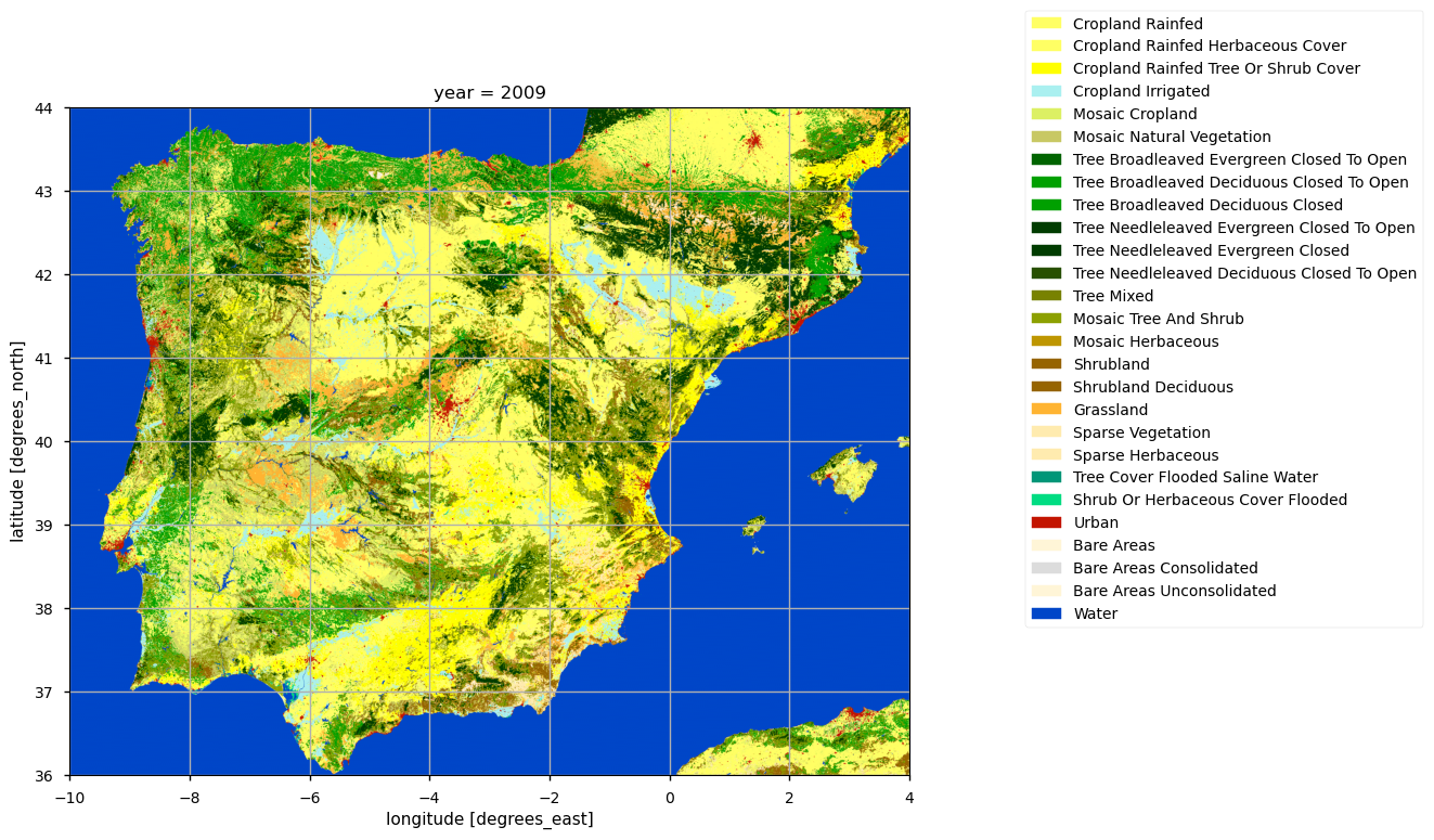
{'No Data': ('#000000', np.uint8(0)),
 'Cropland Rainfed': ('#ffff64', np.uint8(10)),
 'Cropland Rainfed Herbaceous Cover': ('#ffff64', np.uint8(11)),
 'Cropland Rainfed Tree Or Shrub Cover': ('#ffff00', np.uint8(12)),
 'Cropland Irrigated': ('#aaf0f0', np.uint8(20)),
 'Mosaic Cropland': ('#dcf064', np.uint8(30)),
 'Mosaic Natural Vegetation': ('#c8c864', np.uint8(40)),
 'Tree Broadleaved Evergreen Closed To Open': ('#006400', np.uint8(50)),
 'Tree Broadleaved Deciduous Closed To Open': ('#00a000', np.uint8(60)),
 'Tree Broadleaved Deciduous Closed': ('#00a000', np.uint8(61)),
 'Tree Broadleaved Deciduous Open': ('#aac800', np.uint8(62)),
 'Tree Needleleaved Evergreen Closed To Open': ('#003c00', np.uint8(70)),
 'Tree Needleleaved Evergreen Closed': ('#003c00', np.uint8(71)),
 'Tree Needleleaved Evergreen Open': ('#005000', np.uint8(72)),
 'Tree Needleleaved Deciduous Closed To Open': ('#285000', np.uint8(80)),
 'Tree Needleleaved Deciduous Closed': ('#285000', np.uint8(81)),
 'Tree Needleleaved Deciduous Open': ('#286400', np.uint8(82)),
 'Tree Mixed': ('#788200', np.uint8(90)),
 'Mosaic Tree And Shrub': ('#8ca000', np.uint8(100)),
 'Mosaic Herbaceous': ('#be9600', np.uint8(110)),
 'Shrubland': ('#966400', np.uint8(120)),
 'Shrubland Evergreen': ('#966400', np.uint8(121)),
 'Shrubland Deciduous': ('#966400', np.uint8(122)),
 'Grassland': ('#ffb432', np.uint8(130)),
 'Lichens And Mosses': ('#ffdcd2', np.uint8(140)),
 'Sparse Vegetation': ('#ffebaf', np.uint8(150)),
 'Sparse Tree': ('#ffc864', np.uint8(151)),
 'Sparse Shrub': ('#ffd278', np.uint8(152)),
 'Sparse Herbaceous': ('#ffebaf', np.uint8(153)),
 'Tree Cover Flooded Fresh Or Brakish Water': ('#00785a', np.uint8(160)),
 'Tree Cover Flooded Saline Water': ('#009678', np.uint8(170)),
 'Shrub Or Herbaceous Cover Flooded': ('#00dc82', np.uint8(180)),
 'Urban': ('#c31400', np.uint8(190)),
 'Bare Areas': ('#fff5d7', np.uint8(200)),
 'Bare Areas Consolidated': ('#dcdcdc', np.uint8(201)),
 'Bare Areas Unconsolidated': ('#fff5d7', np.uint8(202)),
 'Water': ('#0046c8', np.uint8(210)),
 'Snow And Ice': ('#ffffff', np.uint8(220))}

Show code cell source

Hide code cell source

# Define IPCC labels dictionary
ipcc_dict = {
    "No Data": ("#000000", [0]),
    "Agriculture": ("#ffffcc", [10, 11, 12, 20, 30, 40]),
    "Forest": ("#4c9900", [50, 60, 61, 62, 70, 71, 72, 80, 81, 82, 90, 100, 160, 170]),
    "Grassland": ("#ccff99", [110, 130]),
    "Settlement": ("#ff0000", [190]),
    "Wetland": ("#99ffff", [180]),
    "Other": ("#0000ff", [120, 121, 122, 140, 150, 151, 152, 153, 200, 201, 202, 210]),
}

ipcc_dict 

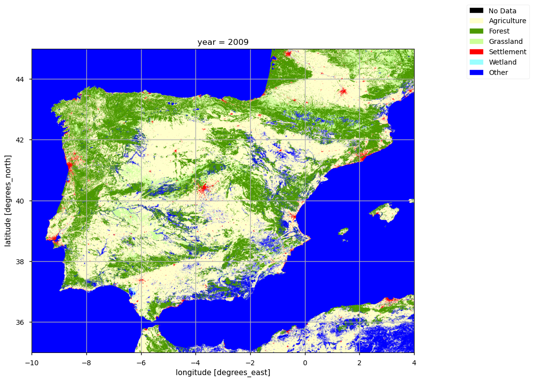
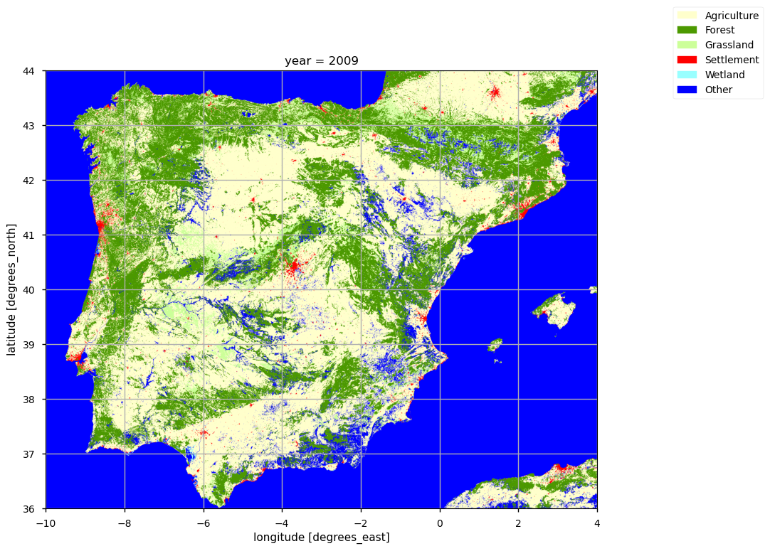
{'No Data': ('#000000', [0]),
 'Agriculture': ('#ffffcc', [10, 11, 12, 20, 30, 40]),
 'Forest': ('#4c9900',
  [50, 60, 61, 62, 70, 71, 72, 80, 81, 82, 90, 100, 160, 170]),
 'Grassland': ('#ccff99', [110, 130]),
 'Settlement': ('#ff0000', [190]),
 'Wetland': ('#99ffff', [180]),
 'Other': ('#0000ff',
  [120, 121, 122, 140, 150, 151, 152, 153, 200, 201, 202, 210])}

Plot maps

Having defined the color and legends for the IPCC classes and using the metadata of the dataset to get the colors and legends for each Land Cover class it is now possible to plot our data either with the original colors or with the IPCC previously defined colors.

The function below plots the LC maps for the year of your choice , using both land cover schemes. From the output, we can already distinguish the differences in classification schemes.

Show code cell source

Hide code cell source

selected_year = 2009 #choose the year you want to inspect
lccs_selected = ds["lccs_class"].sel(year=selected_year)

# unique codes
present_codes = set(map(int, da.unique(lccs_selected.data).compute()))

def filter_lccs_legend_to_present(lccs_dict, present_codes):
    """
    lccs_dict format in your notebook appears to be:
      label -> (color, code)
    We return:
      label -> (color, int(code))   # IMPORTANT: Python int, not numpy scalar
    """
    filtered = {}
    for label, (color, code) in lccs_dict.items():
        code_int = int(code)
        if code_int in present_codes:
            filtered[label] = (color, code_int)
    return filtered

def filter_ipcc_legend_to_present(ipcc_dict, present_codes):
    """
    ipcc_dict format:
      label -> (color, [codes])
    We return codes as a Python list of Python ints, filtered to those present.
    """
    filtered = {}
    for label, (color, codes) in ipcc_dict.items():
        codes_present = [int(c) for c in codes if int(c) in present_codes]
        if codes_present:
            filtered[label] = (color, codes_present)
    return filtered

# Filter both legends
lccs_present_legend = filter_lccs_legend_to_present(lccs_dict, present_codes)
ipcc_present_legend = filter_ipcc_legend_to_present(ipcc_dict, present_codes)

# 1) LCCS map (only present classes in legend)
plt.figure(figsize=(10, 8))
plot.lccs_map(lccs_selected, legend_dict=lccs_present_legend, interpolation="antialiased", figsize=(10, 8))
plt.show()
plt.close()

# 2) IPCC map (only present groups in legend)
plt.figure(figsize=(10, 8))
plot.lccs_map(lccs_selected, legend_dict=ipcc_present_legend, interpolation="antialiased", figsize=(10, 8))
plt.show()
plt.close()

<Figure size 1000x800 with 0 Axes>

<Figure size 1000x800 with 0 Axes>

3. Data preparation and area-based calculations

To further identify changes in LC patterns, in this user question, Nomenclature of Territorial Units for Statistics (NUTS) 2 will be used, providing the information regarding the main regions/parcels of the Iberian Peninsula.

The NUTS are a hierarchical system divided into 3 levels. NUTS 1 correspond to major socio-economic regions, NUTS 2 correspond to basic regions for the application of regional policies, and NUTS 3 correspond to small regions for specific diagnoses. Additionally a NUTS 0 level, usually co-incident with national boundaries is also available. The NUTS legislation is periodically amended; therefore multiple years are available for download.

The step below masks the Land Cover data according to the NUTS 2 boundaries and calculates the area of each pixel (weighted by Latitude). For each NUTS 2 region, we proceed with the analysis and visual inspection of Land Cover areas per class and corresponding percentages during the selected period.

Mask regions

First, we need to establish the geometry of the NUTS region (level 2) in order to make the corresponding statistics.

Show code cell source

Hide code cell source

# Shapefile with regions (NUTS2)
shapefile_url = "https://gisco-services.ec.europa.eu/distribution/v2/nuts/shp/NUTS_RG_20M_2021_4326.shp.zip" #NUTS2 download path

Show code cell source

Hide code cell source

# Define the CRS for the Iberian Peninsula (WGS84)
crs = "epsg:4326"  # EPSG code for WGS84 (latitude/longitude)

# Data filter: load the shapefile and filter for NUTS2 regions in Spain and Portugal
gdf = gpd.read_file(shapefile_url)  # Read the shapefile NUTS2
gdf = gdf[gdf["LEVL_CODE"] == 2]  # Keep only features at the second administrative level (NUTS2)
gdf = gdf[gdf["NUTS_ID"].str.startswith(("ES", "PT"))]  # Keep only NUTS2 regions for Spain (ES) and Portugal (PT)
gdf = gdf.to_crs(crs)  # Ensure CRS is consistent with the dataset

# Create a mask for the NUTS2 regions that intersect with the Iberian Peninsula
regions = regionmask.from_geopandas(gdf, names="NUTS_NAME")  # Create regions mask based on GeoPandas DataFrame

# Apply the mask to the dataset
mask = regions.mask(ds["longitude"], ds["latitude"])

# Only keep land areas (not ocean) by applying the mask
# This ensures that only land pixels are used in the area calculations
ds = ds.where(mask.notnull(), drop=True)  # Drop ocean pixels that are outside the NUTS2 regions

Compute cell area

Then, we can calculate the area of each pixel taking into consideration the curvature of the earth (i.e., weighted by Latitude).

If you want to know more

Show code cell source

Hide code cell source

# Calculate Pixel Area after applying the mask
scaling_factor = 0.002778  # Define a scaling factor for conversion
resolution_km = scaling_factor * 111.195  # Calculate the grid cell resolution in kilometers
indexes = xr.DataArray(range(ds.sizes["latitude"]), dims="latitude")  # Create an array of latitude indexes
lats = ds["latitude"].max() - indexes * scaling_factor
grid_cell_area = resolution_km**2 * np.cos(np.radians(lats))
grid_cell_area.attrs = {
    "standard_name": "cell_area",
    "long_name": "Area",
    "units": "km2",
}
ds = ds.assign_coords(cell_area=grid_cell_area)

4. Analysis and visualisation of Iberian Peninsula land cover changes

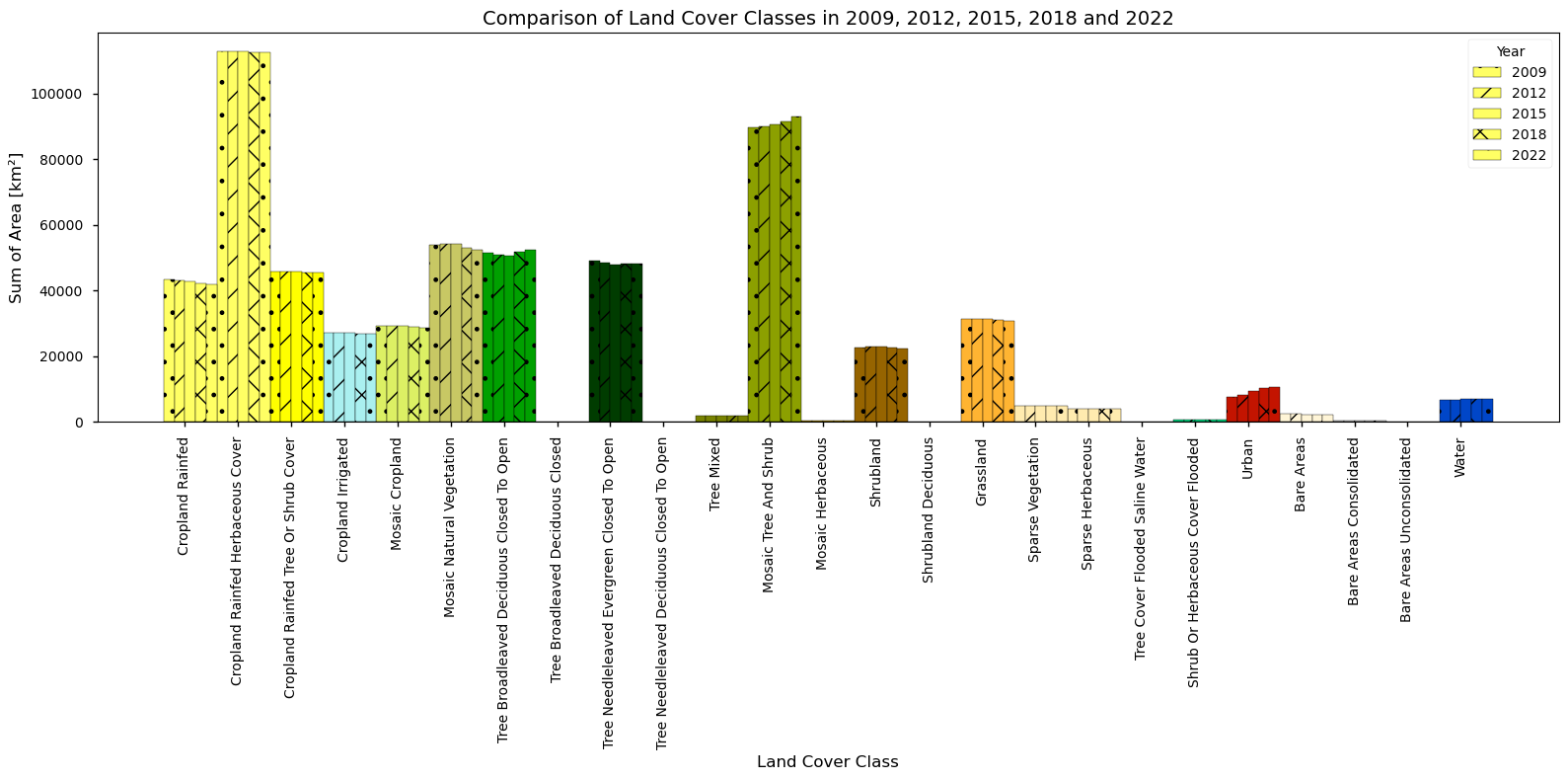
Bar Charts

Having the area calculated and the NUTS 2 regions assigned to each pixel, we can now proceed to create the plots of the LC areas per class, by year. First, let’s inspect the total area of each LC class in this AoI. We will use the original LC classes to highlight which ones show more changes.

Show code cell source

Hide code cell source

# Fuction to calculate class area with original classes
def calculate_area_by_class(ds, cell_area, year):
    # Select the data for the given year
    ds_year = ds.sel(year=year)
    
    # Initialize a dictionary to store the area for each land cover class
    area_by_class = {}
    
    # Loop over each unique land cover class (lccs_class)
    for lc_class in np.unique(ds_year['lccs_class'].values):
        # Create a mask for the current LC class
        mask = ds_year['lccs_class'] == lc_class
        
        # Calculate the total area for the current LC class
        total_area = cell_area.where(mask).sum().compute()  # Use .compute() to get the result
        area_by_class[lc_class] = total_area
    
    return area_by_class

# Calculate areas for 1992 and 2022
area_2009 = calculate_area_by_class(ds, ds["cell_area"], 2009)
area_2012 = calculate_area_by_class(ds, ds["cell_area"], 2012)
area_2015 = calculate_area_by_class(ds, ds["cell_area"], 2015)
area_2018 = calculate_area_by_class(ds, ds["cell_area"], 2018)
area_2022 = calculate_area_by_class(ds, ds["cell_area"], 2022)

Show code cell source

Hide code cell source

# Combine area dictionaries into a single dictionary
area_by_year = {
    2009: area_2009,
    2012: area_2012,
    2015: area_2015,
    2018: area_2018,
    2022: area_2022
}

# Ensure lc_classes excludes NaN
lc_classes = [lc_class for lc_class in np.unique(ds["lccs_class"].values) if not np.isnan(lc_class)]

# Prepare area lists for plotting
area_lists = {
    year: [area_by_year[year].get(lc_class, 0) for lc_class in lc_classes]
    for year in area_by_year
}

# Get class names and colors from the mapping dictionaries
numeric_to_name = {value[1]: key for key, value in lccs_dict.items()}
numeric_to_color = {value[1]: value[0] for key, value in lccs_dict.items()}
class_names = [numeric_to_name.get(int(lc_class), 'Unknown') for lc_class in lc_classes]
colors = [numeric_to_color.get(int(lc_class), '#000000') for lc_class in lc_classes]

# Bar plot settings
bar_width = 0.2
index = np.arange(len(lc_classes))
plt.figure(figsize=(16, 8))

# Unique hatching patterns for visual separation by year
hatch_patterns = {
    2009: '.',
    2012: '/',
    2015: '',
    2018: 'x',
    2022: '.'
}

# Plot bars for each year
for i, year in enumerate(sorted(area_by_year)):
    plt.bar(
        index + i * bar_width,
        area_lists[year],
        bar_width,
        label=str(year),
        color=colors,
        edgecolor='black',
        alpha=1,
        hatch=hatch_patterns[year]
    )

# Final plot customization
plt.xlabel('Land Cover Class', fontsize=12)
plt.ylabel('Sum of Area [km²]', fontsize=12)
plt.title('Comparison of Land Cover Classes in 2009, 2012, 2015, 2018 and 2022', fontsize=14)
plt.xticks(index + bar_width * 1.5, class_names, rotation=90)
plt.legend(title='Year')
plt.tight_layout()
plt.show()

Sankey Diagrams

In this section we take the land-cover maps for consecutive years and quantify how much area changes from one category to another. For each time step (e.g., 2009→2012, 2012→2015, 2015→2018), every grid cell is compared between the two years. If the class changes, we add that cell’s area (km²) to the corresponding “from → to” transition. This produces a table of transitions in km² for each period. The transitions are then aggregated to broader IPCC land-cover groups (e.g., Forest, Cropland, Grassland, Settlements, etc.) so the results are easier to interpret. Finally, these aggregated transitions are visualised as Sankey diagrams.

Each Sankey diagram corresponds to one period (for example 2009→2012). The left side lists the IPCC groups in the first year and the right side lists the IPCC groups in the second year. The ribbons represent land that changed from one group to another; the thickness of a ribbon is the area that changed (km²). Hovering a ribbon shows the same area in km² and also the percentage of the source group’s total change that went to that destination. Only changes between different groups are shown.

Show code cell source

Hide code cell source

# Weighted class transitions (km²) for consecutive years
def compute_pair_transitions_km2(
    ds,
    lccs_var="lccs_class",
    year_var="year",
    area_var="cell_area",
    nodata_code=0,
):
    """
    Compute weighted class→class transition matrices (km²) for each consecutive year pair.

    Returns
    -------
    transitions_km2 : dict[(y0,y1) -> xr.DataArray]
        Each matrix dims: (from_class, to_class), values in km²
    valid_classes : np.ndarray[int]
        Class codes included (nodata removed)
    year_pairs : list[tuple[int,int]]
        Consecutive year pairs
    """
    lccs = ds[lccs_var]
    years = ds[year_var].values.astype(int).tolist()
    year_pairs = list(zip(years[:-1], years[1:]))

    # Broadcast 1D or 2D area -> (lat, lon) like a single year slice
    area_km2_2d = ds[area_var].broadcast_like(lccs.isel({year_var: 0}))

    # Class codes from CF-style flags; exclude nodata_code
    all_codes = np.asarray(lccs.flag_values).astype(int)
    valid_classes = np.array(
        sorted([int(c) for c in all_codes if int(c) != int(nodata_code)]),
        dtype=np.int64,
    )
    nC = int(valid_classes.size)
    max_code = int(all_codes.max())

    # LUT: raw code -> contiguous [0..nC-1], else -1
    lut = -np.ones(max_code + 1, dtype=np.int16)
    lut[valid_classes] = np.arange(nC, dtype=np.int16)

    def _map_codes_to_idx(a_da):
        """Map raw class codes (float with NaNs possible) -> contiguous indices via LUT, dask-safe."""
        def _map_block(block, lut=lut, max_code=max_code):
            finite = np.isfinite(block)
            out = np.full(block.shape, -1, dtype=np.int16)
            if not finite.any():
                return out

            xi = np.empty(block.shape, dtype=np.int64)
            xi[finite] = block[finite].astype(np.int64, copy=False)

            valid = finite & (xi >= 0) & (xi <= max_code)
            if valid.any():
                out[valid] = lut[xi[valid]]
            return out

        return da.map_blocks(_map_block, a_da, dtype=np.int16)

    def _pair_matrix(y0, y1):
        a0 = lccs.sel({year_var: y0}).data
        a1 = lccs.sel({year_var: y1}).data
        w  = area_km2_2d.data

        idx0 = _map_codes_to_idx(a0)
        idx1 = _map_codes_to_idx(a1)

        valid = (idx0 >= 0) & (idx1 >= 0) & da.isfinite(w) & (w > 0)

        i0 = da.where(valid, idx0, -1).ravel()
        i1 = da.where(valid, idx1, -1).ravel()
        ww = da.where(valid, w, 0.0).ravel()

        flat = i0.astype(np.int64) * nC + i1.astype(np.int64)
        sel = i0 >= 0
        flat_valid = flat[sel]
        w_valid = ww[sel]

        bc = da.bincount(flat_valid, weights=w_valid, minlength=nC * nC)
        C = bc.reshape((nC, nC)).compute()  # km²

        return xr.DataArray(
            C,
            coords={"from_class": valid_classes, "to_class": valid_classes},
            dims=("from_class", "to_class"),
            name=f"transitions_{y0}_{y1}_km2",
        )

    transitions_km2 = {(y0, y1): _pair_matrix(y0, y1) for (y0, y1) in year_pairs}
    return transitions_km2, valid_classes, year_pairs


# Aggregate class→class transitions to IPCC groups

def aggregate_transitions_to_ipcc(
    transitions_km2,
    valid_classes,
    ipcc_dict,
    include_nodata_in_groups=False,
):
    """
    Aggregate class→class transition matrices into IPCC groups using membership matrix M.

    ipcc_dict expected shape:
        { group_name: (meta_or_color, [class_codes...]), ... }

    Returns
    -------
    transitions_km2_ipcc : dict[(y0,y1) -> xr.DataArray]
        dims: (from_group, to_group)
    group_order : list[str]
    class_to_group : dict[int -> str]
    """
    class_to_group = {}
    group_order = []

    for g, (_meta, codes) in ipcc_dict.items():
        if g == "No Data" and not include_nodata_in_groups:
            continue
        group_order.append(g)
        for c in codes:
            class_to_group[int(c)] = g

    nC = int(valid_classes.size)
    nG = int(len(group_order))

    code_to_idx = {int(c): i for i, c in enumerate(valid_classes)}

    # Membership matrix M: (nC x nG)
    M = np.zeros((nC, nG), dtype=np.float64)
    for j, g in enumerate(group_order):
        for c in ipcc_dict[g][1]:
            ci = code_to_idx.get(int(c))
            if ci is not None:
                M[ci, j] = 1.0

    def _agg(C_da):
        G_np = M.T @ C_da.values @ M
        return xr.DataArray(
            G_np,
            coords={"from_group": group_order, "to_group": group_order},
            dims=("from_group", "to_group"),
            name=C_da.name.replace("_km2", "_km2_ipcc"),
        )

    transitions_km2_ipcc = {k: _agg(v) for k, v in transitions_km2.items()}
    return transitions_km2_ipcc, group_order, class_to_group


#  Sankey: km² + ONLY % of source outflow; 

def plot_ipcc_sankey_outflow_pct(
    pair,
    transitions_km2_ipcc,
    ignore_self=True,
    min_value_km2=0.0,
    title_suffix="",
    show_source_totals_in_labels=False,  # <- CHANGED default: don't show totals
    disable_node_hover=True,            # <- NEW: no hover on lateral bars
    width=900,
    height=600,
):
    """
    Sankey for one (y0,y1) pair.

    - Link width: km² (area)
    - Link hover: km² + % of *source class outflow* (row-normalised)
    - Node hover disabled by default (no tooltips on lateral bars)
    - Totals in source labels disabled by default
    """
    y0, y1 = pair
    G = transitions_km2_ipcc.get(pair)
    if G is None:
        print(f"[warn] No matrix for pair {pair}")
        return None

    A = G.values.astype(float)  # km²
    rows = list(G.coords["from_group"].values)
    cols = list(G.coords["to_group"].values)
    n = len(rows)

    # Denominator for outflow %: sum of non-self transitions per source row (if ignore_self)
    A_den = A.copy()
    if ignore_self:
        np.fill_diagonal(A_den, 0.0)

    row_outflow = A_den.sum(axis=1, keepdims=True)  # (n,1)

    # Labels: optionally show totals for sources (outflow only)
    if show_source_totals_in_labels:
        src_labels = [
            f"{g}<br>{row_outflow[i,0]:,.0f} km² changed"
            for i, g in enumerate(rows)
        ]
    else:
        src_labels = rows

    labels = src_labels + cols

    sources, targets, values, hover = [], [], [], []

    for i, src in enumerate(rows):
        denom = float(row_outflow[i, 0])

        for j, dst in enumerate(cols):
            if ignore_self and src == dst:
                continue

            km2 = float(A[i, j])
            if (not np.isfinite(km2)) or (km2 <= float(min_value_km2)):
                continue

            pct_out = (km2 / denom * 100.0) if denom > 0 else 0.0

            sources.append(i)
            targets.append(n + j)
            values.append(km2)

            hover.append(
                f"{src} → {dst}<br>"
                f"{km2:,.1f} km²<br>"
                f"{pct_out:.1f}% of {src} outflow"
            )

    if not values:
        print(f"[warn] No transitions above {min_value_km2} km² for {pair}")
        return None

    # Node hover suppression (no tooltips on nodes)
    if disable_node_hover:
        node_dict = dict(
            label=labels,
            pad=15,
            thickness=20,
            line=dict(color="black", width=0.5),
            customdata=[""] * len(labels),
            hovertemplate="<extra></extra>",
        )
    else:
        node_dict = dict(
            label=labels,
            pad=15,
            thickness=20,
            line=dict(color="black", width=0.5),
        )

    fig = go.Figure(
        go.Sankey(
            arrangement="snap",
            node=node_dict,
            link=dict(
                source=sources,
                target=targets,
                value=values,
                customdata=hover,
                hovertemplate="%{customdata}<extra></extra>",
            ),
        )
    )

    title = f"LC Transitions {y0}→{y1}"
    if title_suffix:
        title += f" — {title_suffix}"

    fig.update_layout(title_text=title, font_size=12, width=width, height=height)
    return fig

Show code cell source

Hide code cell source

# Coloring graphs
def hex_to_rgba(hex_color, alpha=0.45):
    """Convert hex colour to rgba string for Sankey links."""
    hex_color = hex_color.lstrip("#")
    r = int(hex_color[0:2], 16)
    g = int(hex_color[2:4], 16)
    b = int(hex_color[4:6], 16)
    return f"rgba({r},{g},{b},{alpha})"


def get_ipcc_colors(ipcc_dict):
    """Extract IPCC class colours from ipcc_dict."""
    return {
        class_name: class_info[0]
        for class_name, class_info in ipcc_dict.items()
    }


def get_ipcc_class_from_label(label, ipcc_colors):
    """
    Match Sankey node labels to IPCC class names.
    Works for labels such as:
    - Forest
    - Forest 2009
    - 2009 Forest
    - Forest (2009)
    """
    label = str(label)

    for class_name in ipcc_colors:
        if class_name in label:
            return class_name

    return "Other"


def apply_ipcc_colors_to_sankey(fig, ipcc_dict):
    """Apply IPCC colours from ipcc_dict to Sankey nodes and links."""
    ipcc_colors = get_ipcc_colors(ipcc_dict)

    sankey = fig.data[0]
    labels = list(sankey.node.label)

    node_colors = [
        ipcc_colors.get(
            get_ipcc_class_from_label(label, ipcc_colors),
            ipcc_colors.get("Other", "#808080")
        )
        for label in labels
    ]

    link_colors = [
        hex_to_rgba(
            ipcc_colors.get(
                get_ipcc_class_from_label(labels[source_idx], ipcc_colors),
                ipcc_colors.get("Other", "#808080")
            ),
            alpha=0.45
        )
        for source_idx in sankey.link.source
    ]

    fig.update_traces(
        node=dict(color=node_colors),
        link=dict(color=link_colors),
        selector=dict(type="sankey")
    )

    return fig

Show code cell source

Hide code cell source

# Plot Sankey Diagrams

transitions_km2, valid_classes, year_pairs = compute_pair_transitions_km2(
    ds,
    lccs_var="lccs_class",
    year_var="year",
    area_var="cell_area",
    nodata_code=0,
)

transitions_km2_ipcc, ipcc_groups_order, class_to_group = aggregate_transitions_to_ipcc(
    transitions_km2,
    valid_classes,
    ipcc_dict,
    include_nodata_in_groups=False,
)

for pair in [(2009, 2012), (2012, 2015), (2015, 2018), (2018, 2022)]:
    fig = plot_ipcc_sankey_outflow_pct(
        pair,
        transitions_km2_ipcc,
        ignore_self=True,
        min_value_km2=0.0,
        show_source_totals_in_labels=False,
        disable_node_hover=True,
    )

    if fig:
        fig = apply_ipcc_colors_to_sankey(fig, ipcc_dict)

        fig.update_layout(
            autosize=False,
            width=700,
            height=450,
            margin=dict(l=20, r=20, t=40, b=20)
        )

        fig.show()

Bar chart and Sankey Diagrams Analysis

The land cover comparison across the selected years (2009, 2012, 2015, 2018 and 2022) shows a clear and persistent increase in urban area. The bar chart provides the net view of these changes, showing a steady rise in the Urban class across all years, while other classes change more gradually without abrupt or implausible shifts. This supports the interpretation that the observed urban growth is systematic over time rather than being driven by isolated anomalies.

The Sankey transition diagrams provide further evidence that the observed urban growth follows realistic land-use change pathways. When analysed using the percentage share of each source class outflow, Agriculture→Settlement transitions account for 64.46% (2009–2012) and 65.91% (2012–2015) of total agricultural change in the respective periods. In the later intervals, this proportion decreases to 23.26% (2015–2018) and 13.49% (2018–2022), indicating that although agriculture remains a major contributor to new Settlement area in absolute terms, a smaller share of overall agricultural transitions is directed toward urban expansion in the later years.

Forest→Settlement transitions represent a consistently smaller proportion of total forest outflow, accounting for 3.58%, 6.81%, 15.50%, and 0.87% across the four respective periods. These values indicate that only a limited fraction of forest change results in direct urban conversion. Grassland→Settlement transitions account for 64.72%, 74.35%, 13.46%, and 3.22% of total grassland outflow across the same periods, indicating that a larger share of grassland change was directed toward urban expansion in the earlier periods than in the later years.

These outflow-based transition patterns confirm that urban growth primarily interacts with agricultural and grassland dynamics, while forest areas play a comparatively minor direct role in settlement expansion. This behaviour aligns with Feranec et al. (2010), who show that urbanisation flows predominantly originate from agricultural classes at the European scale. Similarly, Bagan and Yamagata (2014) identify cropland as the principal donor class to urban growth in global city analyses. In the Iberian Peninsula, Fernández-Nogueira and Corbelle-Rico (2018) report that increases in artificial surfaces occurred alongside stable or increasing forest area, further supporting the interpretation that urban growth does not primarily proceed through direct forest conversion.

Overall, the combined bar chart and Sankey analysis indicates that the dataset captures urbanisation patterns that are coherent across time, internally consistent, and aligned with established land-use change processes documented in the literature.

5. Calculate the area percentage and the area percentage change for the most populated regions

Having identified general urbanisation trends in the Iberian Peninsula, we now focus on specific NUTS2 regions in greater detail. These regions were selected based on their inclusion of the largest urban areas in terms of population, according to the Urban Audit Indicators dataset from the European Commission (Eurostat).

The selected NUTS2 regions are:

• Comunidad de Madrid, which includes the city of Madrid (5,098,717 inhabitants in 2022), the capital of Spain;

• Cataluña, which includes Barcelona (3,755,512 inhabitants in 2022);

• Área Metropolitana de Lisboa, which includes Lisbon (1,872,036 inhabitants in 2022), the capital of Portugal;

• Comunitat Valenciana, which includes Valencia (1,417,464 inhabitants in 2022);

• Norte, which includes Porto (955,864 inhabitants in 2022).

For each of these regions, we analyse land cover dynamics in terms of area percentages by IPCC classes, in order to highlight broader, aggregated land cover changes. Additionally, we compare dataset results with EUROSTAT statistics to assess the consistency between datasets.

Calculation of the percentage area, absolute change, and relative percentage change for each IPCC class category

1. Area Percentage Coverage:
   Example: In 1992, forest land covered 35% of the total area, while urban areas occupied 10%. By 2022, forest coverage decreased to 30%, and urban areas expanded to 15%. This metric gives the proportion of the total land occupied by each land cover class.

2. Absolute Percentage Difference:
   Example: In 1992, 10% of the region was classified as agricultural land. By 2022, this had decreased to 8%. The absolute percentage difference in agricultural land coverage is −2% (from 10% in 1992 to 8% in 2022, representing a 2% decrease in total land area occupied by agriculture).

3. Relative Percentage Difference:
   Example: In 1992, 10% of the area was classified as wetlands. By 2022, wetlands accounted for 12% of the total area. The relative percentage difference is calculated as ((12−10)/10)∗100 = +20%. This means there was a 20% increase in wetland area relative to its size in 1992.

Show code cell source

Hide code cell source

# Filter the GeoDataFrame to include only the regions of interest
regions= ["Comunidad de Madrid", "Cataluña", "Área Metropolitana de Lisboa", "Comunitat Valenciana", "Norte"]

gdf_filtered = gdf[gdf['NUTS_NAME'].isin(regions)]
gdf_filtered = gdf_filtered.to_crs("EPSG:4326")

# Expand cell_area ONCE outside the loops
cell_area = ds["cell_area"].expand_dims({"longitude": ds.sizes["longitude"]}, axis=1)

# Prepare latitude and longitude grids ONCE
lat, lon = ds['latitude'].values, ds['longitude'].values
lon_grid, lat_grid = np.meshgrid(lon, lat)  # avoid recalculating inside mask function

Show code cell source

Hide code cell source

# Create region mask using shapely
def create_region_mask(region_geom, lon_grid, lat_grid):
    points = [shapely.geometry.Point(x, y) for x, y in zip(lon_grid.ravel(), lat_grid.ravel())]
    mask = np.array([region_geom.contains(pt) for pt in points]).reshape(lon_grid.shape)
    return xr.DataArray(mask, coords=[lat, lon], dims=["latitude", "longitude"])

# Calculate IPCC class % coverage for a given year and region
def calculate_ipcc_coverage(year, region_mask, cell_area, ipcc_dict, total_area):
    lccs = ds["lccs_class"].sel(year=year).where(region_mask)
    return {
        group: ((xr.where(np.isin(lccs, codes), 1, 0) * cell_area).sum().item() / total_area) * 100
        for group, (_, codes) in ipcc_dict.items()
    }

# Compute absolute and relative differences
def compute_differences(base, target):
    abs_diff = {k: target[k] - base[k] for k in base}
    rel_diff = {k: ((target[k] - base[k]) / base[k]) * 100 if base[k] else 0 for k in base}
    return abs_diff, rel_diff

# Padded y-axis limits
def padded_limits(values, pad=0.1):
    finite_vals = [v for v in values if np.isfinite(v)]
    if not finite_vals: return 0, 1
    min_v, max_v = min(finite_vals), max(finite_vals)
    return min_v, max_v + (max_v - min_v) * pad

Show code cell source

Hide code cell source

# Ploting fuctions 
def plot_coverage(ax, cov_2009, cov_2022, region, ymax):
    labels = [k for k in cov_2009 if k != 'No Data']
    x = np.arange(len(labels))
    width = 0.35
    colors = [ipcc_dict[k][0] for k in labels]
    y1 = [cov_2009[k] for k in labels]
    y2 = [cov_2022[k] for k in labels]

    ax.bar(x - width/2, y1, width, color=colors, edgecolor='black', label='2009')
    ax.bar(x + width/2, y2, width, color=colors, edgecolor='black', hatch='//', label='2022')
    ax.set_ylabel('Coverage Area (%)')
    ax.set_title(f'"{region}" NUTS2')
    ax.set_xticks(x)
    ax.set_xticklabels(labels, rotation=45, ha='right')
    ax.set_ylim(0, ymax)
    ax.grid(True, linestyle='--', alpha=0.6)
    ax.legend()

# Plot absolute and relative differences (side-by-side bars)
def plot_differences(ax1, ax2, abs_d, rel_d, region, lims_abs, lims_rel):
    labels = [k for k in abs_d if k != 'No Data']
    x = np.arange(len(labels))
    width = 0.35
    colors = [ipcc_dict[k][0] for k in labels]

    # Absolute difference
    ax1.bar(x, [abs_d[k] for k in labels], width, color=colors, edgecolor='black')
    ax1.set_ylabel('Absolute Change (%)')
    ax1.set_title(f'Abs Diff "{region}"')
    ax1.set_xticks(x)
    ax1.set_xticklabels(labels, rotation=45, ha='right')
    ax1.set_ylim(*lims_abs)
    ax1.grid(True, linestyle='--', alpha=0.6)

    # Relative difference
    ax2.bar(x, [rel_d[k] for k in labels], width, color=colors, edgecolor='black')
    ax2.set_ylabel('Relative Change (%)')
    ax2.set_title(f'Rel Diff "{region}"')
    ax2.set_xticks(x)
    ax2.set_xticklabels(labels, rotation=45, ha='right')
    ax2.set_ylim(*lims_rel)
    ax2.grid(True, linestyle='--', alpha=0.6)

Show code cell source

Hide code cell source

#Plot change
# Year to check
years_to_check = [2009, 2012, 2015, 2018,2022]
global_cov, global_abs, global_rel = [], [], []

# Storage dictionary for later reuse
all_coverages = {}  # (region, year) -> coverage dict

# Calculate everything
for region in regions:
    geom = gdf_filtered[gdf_filtered["NUTS_NAME"] == region].geometry.union_all()
    mask = create_region_mask(geom, lon_grid, lat_grid)
    total_area = (mask * cell_area).sum().item()
    if total_area == 0:
        continue

    for year in years_to_check:
        cov = calculate_ipcc_coverage(year, mask, cell_area, ipcc_dict, total_area)
        all_coverages[(region, year)] = cov

    # For plotting (only cov_2009 vs cov_2022)
    cov_2009 = all_coverages[(region, 2009)]
    cov_2022 = all_coverages[(region, 2022)]
    abs_d, rel_d = compute_differences(cov_2009, cov_2022)

    global_cov.extend(list(cov_2009.values()) + list(cov_2022.values()))
    global_abs.extend(abs_d.values())
    global_rel.extend(rel_d.values())

# Calculate global plot limits
lims_cov = padded_limits(global_cov)
lims_abs = padded_limits(global_abs)
lims_rel = padded_limits(global_rel)


# Plot results
for region in regions:
    cov_2009 = all_coverages[(region, 2009)]
    cov_2022 = all_coverages[(region, 2022)]
    abs_d, rel_d = compute_differences(cov_2009, cov_2022)

    fig, (ax1, ax2, ax3) = plt.subplots(1, 3, figsize=(18, 5))
    plot_coverage(ax1, cov_2009, cov_2022, region, lims_cov[1])
    plot_differences(ax2, ax3, abs_d, rel_d, region, lims_abs, lims_rel)
    plt.tight_layout()
    plt.show()

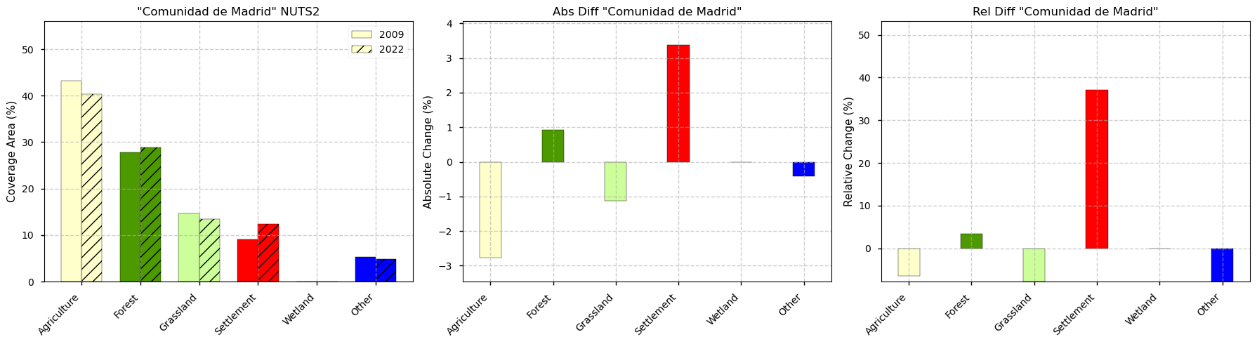
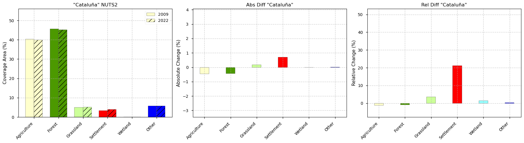
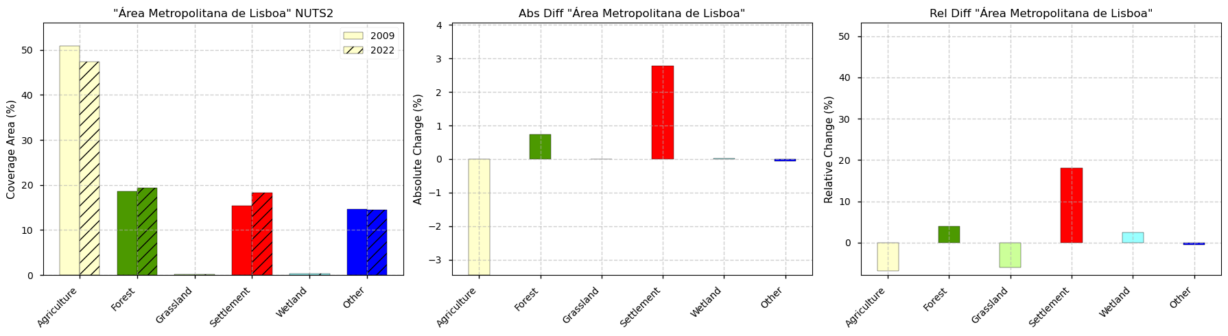
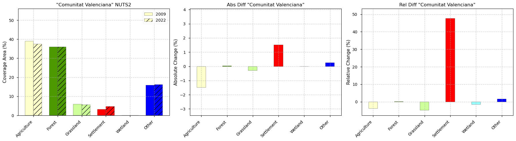
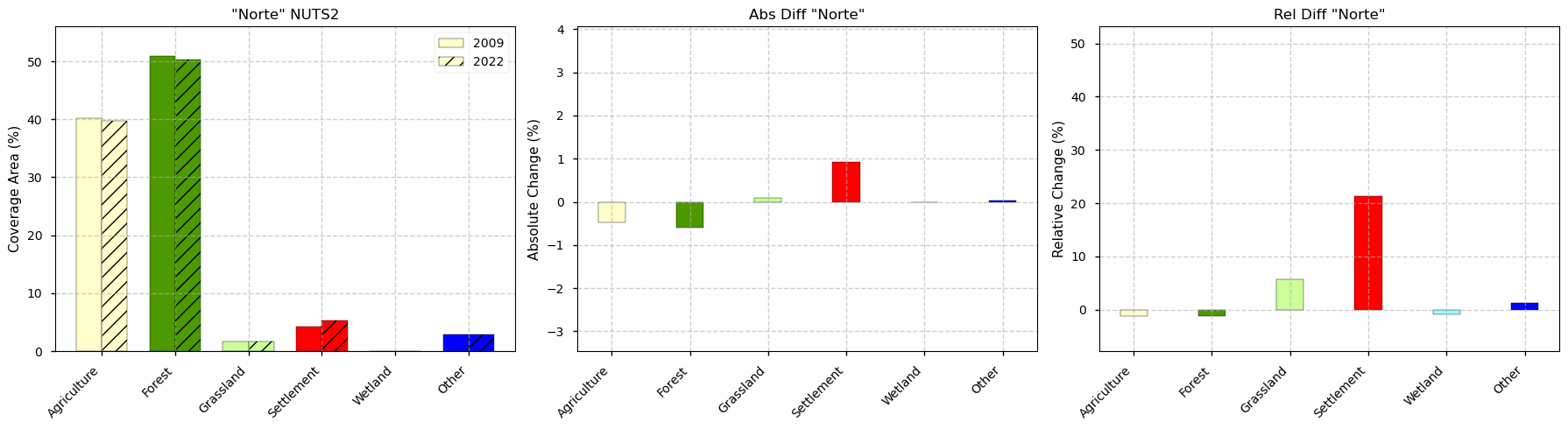
Bar Chart Analysis

Across the five most populated NUTS2 regions clear land cover change patterns are observed between 2009 and 2022, especially in relation to urban expansion and agricultural decline.

• Settlement/Urban areas show a consistent increase in all regions, with the most pronounced growth occurring in Área Metropolitana de Lisboa and Comunidad de Madrid.

• Agricultural land has decreased across all regions, with the sharpest reduction seen in Área Metropolitana de Lisboa. The decline appears moderate in Comunidad de Madrid, Cataluña, and Comunitat Valenciana, suggesting a gradual conversion of agricultural land to urban or other uses.

• Forest and grassland areas remained mostly stable in several regions, with small increases in Comunitat Valenciana and Cataluña, indicating preservation or limited natural regeneration in non‑urbanised areas. However, in Norte and Valencia, forest cover declined despite only a minimal change of agricultural land. This pattern suggests that the reduction in forest area is linked to the expansion of settlements.

• Wetlands and other land cover categories continue to represent a negligible share of total area. Their relative and absolute changes are minimal, with little to no impact on the overall land use structure of the regions.

Comparison with EUROSTAT Data

To validate the consistency of the C3S Land Cover dataset in the context of urbanisation, we compared the percentage of land classified as Settlement with EUROSTAT artificial land statistics for the five most populated NUTS2 regions in the Iberian Peninsula. In addition, key non-urban land cover classes—Forest, Grassland, and Agriculture—are included in the comparison to provide context for the land cover changes associated with urban expansion.

EUROSTAT land-cover and land-use statistics are based on the LUCAS survey, an in-situ survey in which field surveyors classify the observed land cover and visible land use at sampled points using harmonised LUCAS classifications. LUCAS explicitly separates land cover, meaning the physical cover of the Earth’s surface, from land use, meaning the socio-economic function of the land. The LUCAS land-cover classification is hierarchical and includes A00 Artificial land as one of the main land-cover categories.

In the LUCAS classification, the settlement/artificial-surface category is constructed from the following land-cover classes:

• A10 Roofed built-up areas, including buildings and greenhouses;

• A20 Artificial non built-up areas, including sealed area features such as yards, farmyards, cemeteries and car parking areas, as well as linear features such as streets, roads, railways and runways;

• A30 Other artificial areas, including bridges and viaducts, mobile homes, solar panels, power plants, electrical substations, pipelines, sewage plants and open dump sites.

The table below presents values for the five years for which EUROSTAT land cover data are available (2009, 2012, 2015, 2018 and 2022).

Show code cell source

Hide code cell source

# EUROSTAT reference values (percent)

eurostat_artificial = {
    ("Área Metropolitana de Lisboa", 2009): 14.6,
    ("Área Metropolitana de Lisboa", 2012): 15.4,
    ("Área Metropolitana de Lisboa", 2015): 15.8,
    ("Área Metropolitana de Lisboa", 2018): 18.9,
    ("Área Metropolitana de Lisboa", 2022): 17.7,
    ("Comunidad de Madrid", 2009): 9.7,
    ("Comunidad de Madrid", 2012): 10.1,
    ("Comunidad de Madrid", 2015): 10.6,
    ("Comunidad de Madrid", 2018): 11.7,
    ("Comunidad de Madrid", 2022): 11.5,
    ("Cataluña", 2009): 6.3,
    ("Cataluña", 2012): 6.4,
    ("Cataluña", 2015): 6.5,
    ("Cataluña", 2018): 5.3,
    ("Cataluña", 2022): 5.9,
    ("Comunitat Valenciana", 2009): 6.1,
    ("Comunitat Valenciana", 2012): 6.2,
    ("Comunitat Valenciana", 2015): 6.5,
    ("Comunitat Valenciana", 2018): 7.2,
    ("Comunitat Valenciana", 2022): 6.9,
    ("Norte", 2009): 6.8,
    ("Norte", 2012): 6.9,
    ("Norte", 2015): 7.0,
    ("Norte", 2018): 9.4,
    ("Norte", 2022): 8.0,
}

eurostat_woodland = {
    ("Área Metropolitana de Lisboa", 2009): 11.4,
    ("Área Metropolitana de Lisboa", 2012): 22.1,
    ("Área Metropolitana de Lisboa", 2015): 23.2,
    ("Área Metropolitana de Lisboa", 2018): 28.1,
    ("Área Metropolitana de Lisboa", 2022): 24.5,
    ("Comunidad de Madrid", 2009): 15.3,
    ("Comunidad de Madrid", 2012): 20.1,
    ("Comunidad de Madrid", 2015): 24.1,
    ("Comunidad de Madrid", 2018): 30.6,
    ("Comunidad de Madrid", 2022): 32.1,
    ("Cataluña", 2009): 41.5,
    ("Cataluña", 2012): 44.8,
    ("Cataluña", 2015): 44.8,
    ("Cataluña", 2018): 49.6,
    ("Cataluña", 2022): 48.2,
    ("Comunitat Valenciana", 2009): 23.4,
    ("Comunitat Valenciana", 2012): 29.2,
    ("Comunitat Valenciana", 2015): 29.8,
    ("Comunitat Valenciana", 2018): 35.5,
    ("Comunitat Valenciana", 2022): 34.0,
    ("Norte", 2009): 22.6,
    ("Norte", 2012): 24.1,
    ("Norte", 2015): 26.1,
    ("Norte", 2018): 28.9,
    ("Norte", 2022): 26.7,
}

eurostat_grassland = {
    ("Área Metropolitana de Lisboa", 2009): 21.4,
    ("Área Metropolitana de Lisboa", 2012): 25.7,
    ("Área Metropolitana de Lisboa", 2015): 22.7,
    ("Área Metropolitana de Lisboa", 2018): 16.5,
    ("Área Metropolitana de Lisboa", 2022): 22.2,
    ("Comunidad de Madrid", 2009): 25.3,
    ("Comunidad de Madrid", 2012): 24.4,
    ("Comunidad de Madrid", 2015): 24.9,
    ("Comunidad de Madrid", 2018): 20.4,
    ("Comunidad de Madrid", 2022): 17.9,
    ("Cataluña", 2009): 13.1,
    ("Cataluña", 2012): 12.8,
    ("Cataluña", 2015): 13.4,
    ("Cataluña", 2018): 8.9,
    ("Cataluña", 2022): 9.2,
    ("Comunitat Valenciana", 2009): 13.4,
    ("Comunitat Valenciana", 2012): 14.1,
    ("Comunitat Valenciana", 2015): 14.0,
    ("Comunitat Valenciana", 2018): 5.6,
    ("Comunitat Valenciana", 2022): 6.6,
    ("Norte", 2009): 17.7,
    ("Norte", 2012): 18.2,
    ("Norte", 2015): 16.9,
    ("Norte", 2018): 14.3,
    ("Norte", 2022): 13.3,
}

eurostat_cropland = {
    ("Área Metropolitana de Lisboa", 2009): 18.5,
    ("Área Metropolitana de Lisboa", 2012): 14.9,
    ("Área Metropolitana de Lisboa", 2015): 13.6,
    ("Área Metropolitana de Lisboa", 2018): 17.4,
    ("Área Metropolitana de Lisboa", 2022): 15.9,
    ("Comunidad de Madrid", 2009): 15.5,
    ("Comunidad de Madrid", 2012): 14.0,
    ("Comunidad de Madrid", 2015): 15.6,
    ("Comunidad de Madrid", 2018): 17.7,
    ("Comunidad de Madrid", 2022): 15.1,
    ("Cataluña", 2009): 21.7,
    ("Cataluña", 2012): 19.5,
    ("Cataluña", 2015): 18.4,
    ("Cataluña", 2018): 24.4,
    ("Cataluña", 2022): 19.9,
    ("Comunitat Valenciana", 2009): 11.4,
    ("Comunitat Valenciana", 2012): 14.0,
    ("Comunitat Valenciana", 2015): 12.2,
    ("Comunitat Valenciana", 2018): 25.8,
    ("Comunitat Valenciana", 2022): 25.6,
    ("Norte", 2009): 14.0,
    ("Norte", 2012): 12.2,
    ("Norte", 2015): 11.5,
    ("Norte", 2018): 18.0,
    ("Norte", 2022): 19.1,
}


# Combined table for all classes and years

def eu_get(d, region, year):
    return d.get((region, int(year)), None)

rows = []
for region in regions:
    for year in years_to_check:
        cov = all_coverages.get((region, year))
        if cov is None:
            continue

        row = {
            "Region": region,
            "Year": int(year),
            "C3S Settlement (%)": cov.get("Settlement"),
            "EUROSTAT Artificial (%)": eu_get(eurostat_artificial, region, year),
            "Δ Settlement (%)": None if (cov.get("Settlement") is None or eu_get(eurostat_artificial, region, year) is None)
                                else cov["Settlement"] - eu_get(eurostat_artificial, region, year),
            "C3S Forest (%)": cov.get("Forest"),
            "EUROSTAT Woodland (%)": eu_get(eurostat_woodland, region, year),
            "Δ Forest (%)": None if (cov.get("Forest") is None or eu_get(eurostat_woodland, region, year) is None)
                              else cov["Forest"] - eu_get(eurostat_woodland, region, year),
            "C3S Grassland (%)": cov.get("Grassland"),
            "EUROSTAT Grassland (%)": eu_get(eurostat_grassland, region, year),
            "Δ Grassland (%)": None if (cov.get("Grassland") is None or eu_get(eurostat_grassland, region, year) is None)
                                 else cov["Grassland"] - eu_get(eurostat_grassland, region, year),
            "C3S Agriculture (%)": cov.get("Agriculture"),
            "EUROSTAT Cropland (%)": eu_get(eurostat_cropland, region, year),
            "Δ Agriculture (%)": None if (cov.get("Agriculture") is None or eu_get(eurostat_cropland, region, year) is None)
                                  else cov["Agriculture"] - eu_get(eurostat_cropland, region, year),
        }
        rows.append(row)

df_combined = pd.DataFrame(rows).sort_values(["Region", "Year"]).reset_index(drop=True)

pd.set_option("display.max_rows", None)
print(df_combined.round(2).to_string(index=False))

                      Region  Year  C3S Settlement (%)  EUROSTAT Artificial (%)  Δ Settlement (%)  C3S Forest (%)  EUROSTAT Woodland (%)  Δ Forest (%)  C3S Grassland (%)  EUROSTAT Grassland (%)  Δ Grassland (%)  C3S Agriculture (%)  EUROSTAT Cropland (%)  Δ Agriculture (%)
                    Cataluña  2009                3.29                      6.3             -3.01           45.66                   41.5          4.16               4.98                    13.1            -8.12                40.30                   21.7              18.60
                    Cataluña  2012                3.49                      6.4             -2.91           45.52                   44.8          0.72               4.99                    12.8            -7.81                40.21                   19.5              20.71
                    Cataluña  2015                3.71                      6.5             -2.79           45.42                   44.8          0.62               5.01                    13.4            -8.39                40.08                   18.4              21.68
                    Cataluña  2018                3.93                      5.3             -1.37           45.51                   49.6         -4.09               5.04                     8.9            -3.86                39.79                   24.4              15.39
                    Cataluña  2022                3.98                      5.9             -1.92           45.23                   48.2         -2.97               5.16                     9.2            -4.04                39.84                   19.9              19.94
         Comunidad de Madrid  2009                9.09                      9.7             -0.61           27.87                   15.3         12.57              14.63                    25.3           -10.67                43.16                   15.5              27.66
         Comunidad de Madrid  2012                9.62                     10.1             -0.48           27.71                   20.1          7.61              14.55                    24.4            -9.85                42.83                   14.0              28.83
         Comunidad de Madrid  2015               10.30                     10.6             -0.30           27.44                   24.1          3.34              14.43                    24.9           -10.47                42.51                   15.6              26.91
         Comunidad de Madrid  2018               12.23                     11.7              0.53           28.62                   30.6         -1.98              13.65                    20.4            -6.75                40.58                   17.7              22.88
         Comunidad de Madrid  2022               12.47                     11.5              0.97           28.80                   32.1         -3.30              13.50                    17.9            -4.40                40.39                   15.1              25.29
        Comunitat Valenciana  2009                3.16                      6.1             -2.94           36.00                   23.4         12.60               5.96                    13.4            -7.44                38.93                   11.4              27.53
        Comunitat Valenciana  2012                3.46                      6.2             -2.74           35.29                   29.2          6.09               5.94                    14.1            -8.16                38.62                   14.0              24.62
        Comunitat Valenciana  2015                3.86                      6.5             -2.64           35.45                   29.8          5.65               5.90                    14.0            -8.10                38.19                   12.2              25.99
        Comunitat Valenciana  2018                4.58                      7.2             -2.62           35.66                   35.5          0.16               5.77                     5.6             0.17                37.54                   25.8              11.74
        Comunitat Valenciana  2022                4.67                      6.9             -2.23           36.03                   34.0          2.03               5.67                     6.6            -0.93                37.43                   25.6              11.83
                       Norte  2009                4.33                      6.8             -2.47           50.91                   22.6         28.31               1.63                    17.7           -16.07                40.17                   14.0              26.17
                       Norte  2012                4.68                      6.9             -2.22           50.32                   24.1         26.22               1.70                    18.2           -16.50                40.36                   12.2              28.16
                       Norte  2015                5.08                      7.0             -1.92           49.55                   26.1         23.45               1.79                    16.9           -15.11                40.62                   11.5              29.12
                       Norte  2018                5.14                      9.4             -4.26           50.07                   28.9         21.17               1.77                    14.3           -12.53                39.99                   18.0              21.99
                       Norte  2022                5.25                      8.0             -2.75           50.32                   26.7         23.62               1.73                    13.3           -11.57                39.70                   19.1              20.60
Área Metropolitana de Lisboa  2009               15.46                     14.6              0.86           18.62                   11.4          7.22               0.12                    21.4           -21.28                50.80                   18.5              32.30
Área Metropolitana de Lisboa  2012               16.58                     15.4              1.18           18.58                   22.1         -3.52               0.12                    25.7           -25.58                49.77                   14.9              34.87
Área Metropolitana de Lisboa  2015               17.66                     15.8              1.86           18.62                   23.2         -4.58               0.12                    22.7           -22.58                48.64                   13.6              35.04
Área Metropolitana de Lisboa  2018               18.12                     18.9             -0.78           19.02                   28.1         -9.08               0.11                    16.5           -16.39                47.82                   17.4              30.42
Área Metropolitana de Lisboa  2022               18.25                     17.7              0.55           19.35                   24.5         -5.15               0.11                    22.2           -22.09                47.34                   15.9              31.44

Across all regions, both datasets indicate a systematic increase in urban land over time, with comparable magnitudes and trajectories. Absolute differences in settlement/artificial land percentages are generally small, particularly in highly urbanised regions. For Comunidad de Madrid, differences remain below ±1% throughout the period, while Área Metropolitana de Lisboa shows differences mostly within ±2%, despite its higher overall urban fraction.

In regions with more dispersed or heterogeneous urban structures—such as Cataluña, Comunitat Valenciana, and Norte—C3S settlement values are consistently lower than EUROSTAT artificial land by approximately 1–3%. This offset is stable across years and likely reflects both definitional differences and differences in dataset construction, including spatial resolution. Because C3S is a satellite-derived 300 m gridded product, small or fragmented artificial surfaces may be represented differently from EUROSTAT/LUCAS artificial land, which is based on in-situ point observations aggregated statistically. Crucially, both datasets capture similar rates and directions of urban expansion, indicating that urbanisation dynamics are robustly identified despite these differences.

Between 2009 and 2022, urban land increased in all regions in both datasets, with comparable absolute changes. For example, in Comunidad de Madrid, C3S settlement increased by +3.38 percentage points (from 9.09% to 12.47%), while EUROSTAT artificial land increased by +1.8 percentage points (from 9.7% to 11.5%). Similarly, in Área Metropolitana de Lisboa, C3S reports an increase of +2.79 percentage points, compared to +3.1 percentage points in EUROSTAT. These comparable magnitudes indicate that both datasets capture a similar volume of land converted into urban use.

The land cover losses associated with this urban expansion are also consistent in direction. Across all regions, urban growth coincides primarily with reductions in agricultural and open land classes. For instance, in Cataluña, the cumulative increase in settlement between 2009 and 2022 (approximately +0.7 percentage points in C3S) corresponds to a decrease in agricultural land of around –0.5 percentage points, while EUROSTAT reports a comparable decline in cropland over the same period. Similar patterns are observed in Comunitat Valenciana and Norte, where modest but persistent urban gains are accompanied by declining agricultural shares in both datasets.

Although C3S and EUROSTAT differ in how agricultural, grassland, and mixed-use areas are classified, these differences do not alter the identification of urban-driven land take. Both datasets indicate that urban expansion primarily occurs at the expense of agricultural and open land, while forest areas remain comparatively stable. This agreement confirms that, in terms of urbanisation impact, the datasets provide equivalent signals of land cover loss.

Overall, the comparison demonstrates that the C3S Land Cover dataset is consistent with EUROSTAT in capturing the magnitude and evolution of urban expansion at the NUTS2 level. Minor systematic offsets in absolute values do not compromise the dataset’s suitability for analysing urban growth, land take, and associated land cover loss. For regional-scale monitoring of urbanisation processes, the C3S dataset therefore provides results that are comparable to official statistics, while offering the added benefit of spatially explicit, satellite-based observations.

6. Main Takeaways

• The dataset demonstrates physical consistency with official sources, aligning well with EUROSTAT statistics and previously reported European land-cover analyses (e.g. Feranec et al., 2010; Fernández-Nogueira & Corbelle-Rico, 2018). Between 2009 and 2022, urbanisation occurred across major NUTS2 regions, with settlement areas doubling in some cases. This expansion largely came at the expense of Agriculture and Grassland classes. The observed magnitude and direction of change are consistent with broader European urbanisation trends identified using the GHSL dataset (Alberti et al., 2019). Small discrepancies (<5%) with EUROSTAT artificial land statistics do not compromise the dataset’s reliability for identifying overall land-use change trends, though users focusing on very localised patterns should interpret results with caution.

• Urban expansion mainly replaced agricultural and open land, while Forest areas remained largely stable over the study period. Settlements increased their share of total land area across regions and remain a minority land cover class. These patterns are consistent with spatial trade-off dynamics reported in global urban land-cover change analyses, where urban growth frequently draws from agricultural land rather than direct forest conversion (Bagan & Yamagata, 2014).

• The use of both detailed and aggregated IPCC classes provided a comprehensive view of land cover dynamics, balancing precision and generalisation. Although class aggregation introduces some uncertainty (e.g. between Agriculture and Grassland), it enables clearer identification of dominant transitions such as urban expansion, consistent with structured land-cover change assessment approaches reported in the literature.

• Minor classification differences between datasets (e.g. coding of mixed-use or greenhouse areas) can introduce uncertainty. Nonetheless, the dataset maintains strong performance in identifying urban expansion trends, in line with consistency and accuracy assessments of global land-cover products (Zhao et al., 2023).

ℹ️ If you want to know more

Key resources

Some key resources and further reading were linked throughout this assessment.

The CDS catalogue entry for the data used were:

• Land cover classification gridded maps from 1992 to present derived from satellite observations: (https://cds.climate.copernicus.eu/datasets/satellite-land-cover?tab=overview)

• Product User Guide and Specification of the dataset version 2.1 and version 2.0

Additional resources:

• Eurostat NUTS (Nomenclature of territorial units for statistics)

Code libraries used:

• C3S EQC custom functions, c3s_eqc_automatic_quality_control, prepared by B-Open

References

Feranec, J., Jaffrain, G., Soukup, T., & Hazeu, G. (2010). Determining changes and flows in European landscapes 1990–2000 using CORINE land cover data. Applied geography, 30(1), 19-35.

Fernández-Nogueira, D., & Corbelle-Rico, E. (2018). Land use changes in Iberian Peninsula 1990–2012. Land, 7(3), 99.

Eurostat, Statistical Atlas

Bagan, H., & Yamagata, Y. (2014). Land-cover change analysis in 50 global cities by using a combination of Landsat data and analysis of grid cells. Environmental Research Letters, 9.

Alberti, V., Alonso Raposo, M., Attardo, C., Auteri, D., Ribeiro Barranco, R., Batista E Silva, F., Benczur, P., Bertoldi, P., Bono, F., Bussolari, I., Louro Caldeira, S., Carlsson, J., Christidis, P., Christodoulou, A., Ciuffo, B., Corrado, S., Fioretti, C., Galassi, M., Galbusera, L., Gawlik, B., Giusti, F., Gomez Prieto, J., Grosso, M., Martinho Guimaraes Pires Pereira, A., Jacobs, C., Kavalov, B., Kompil, M., Kucas, A., Kona, A., Lavalle, C., Leip, A., Lyons, L., Manca, A., Melchiorri, M., Monforti-Ferrario, F., Montalto, V., Mortara, B., Natale, F., Panella, F., Pasi, G., Perpiña Castillo, C., Pertoldi, M., Pisoni, E., Roque Mendes Polvora, A., Rainoldi, A., Rembges, D., Rissola, G., Sala, S., Schade, S., Serra, N., Spirito, L., Tsakalidis, A., Schiavina, M., Tintori, G., Vaccari, L., Vandyck, T., Vanham, D., Van Heerden, S., Van Noordt, C., Vespe, M., Vetters, N., Vilahur Chiaraviglio, N., Vizcaino, M., Von Estorff, U. and Zulian, G., The Future of Cities, Vandecasteele, I., Baranzelli, C., Siragusa, A. and Aurambout, J. editor(s), EUR 29752 EN, Publications Office of the European Union, Luxembourg, 2019, ISBN 978-92-76-03847-4, doi:10.2760/375209, JRC116711.

Zhao, T., Zhang, X., Gao, Y., Mi, J., Liu, W., Wang, J., Jiang, M., & Liu, L. (2023). Assessing the Accuracy and Consistency of Six Fine-Resolution Global Land Cover Products Using a Novel Stratified Random Sampling Validation Dataset. Remote. Sens., 15, 2285.