

4.6. Benefit and challenges of a multi-model approach to seasonal forecasts#
Production date: 07-05-2025
Produced by: Sandro Calmanti, Alessandro Dell’Aquila (ENEA)
🌍 Use case: Using multi-model ensembles for seasonal forecast sectoral applications#
❓ Quality assessment questions#
Can I improve the skill of seasonal forecasts by using a multi-model ensemble of climate predictions?
Are there robust strategies for creating multi-model ensembles?
C3S provides a multi-model ensemble of seasonal climate predictions produced by nine forecast centres in Europe, North America, Japan and Australia. The development of a European multi-model ensemble for seasonal forecasting has been supported throughout several research programs ( DEMETER / ENSEMBLES / EUROSIP) which have progressively contributed to the improvement of the underpinning climate models (e.g. [1], [2], [3] ). The multi-model ensemble available through C3S is therefore the outcome of a long lasting endeavour, enriched with similar predictions derived from other non-european forecasting centres.
In principle, it is possible to use the seasonal predictions from different centers as a single multi-model ensemble to increase the reliability and the overall value of the forecast.
However, handling multi-model ensembles to create climate information on a regular basis, is a complex and resource intensive task. This article summarises the significant experiences in working with multi-model ensembles with the objective of highlighting the potential added value, the challenges and limitations in the use of multi-model ensembles
📢 Quality assessment statement#
These are the key outcomes of this assessment
The multi-model ensemble (MME) approach consistently outperforms individual models in terms of skill metrics such as temporal correlation and probabilistic accuracy, particularly when the combined models are developed independently
The use of multi-model ensembles allows for a better assessment of forecast uncertainty and has been shown to support more informed decision-making, especially in hydrological and water resource applications.
The MME approach shows the greatest value in tropical regions, where model errors dominate over initial condition uncertainties, enabling effective bias compensation.
Sectoral applications can benefit from filtering or weighting the most skillful models for a specific region or variable of interest, such as in national wheat yield forecasting or malaria risk.
Bias adjustment and model recalibration are necessary post-processing steps that significantly enhance the reliability of multi-model forecasts, especially when outputs are used as input to impact models.
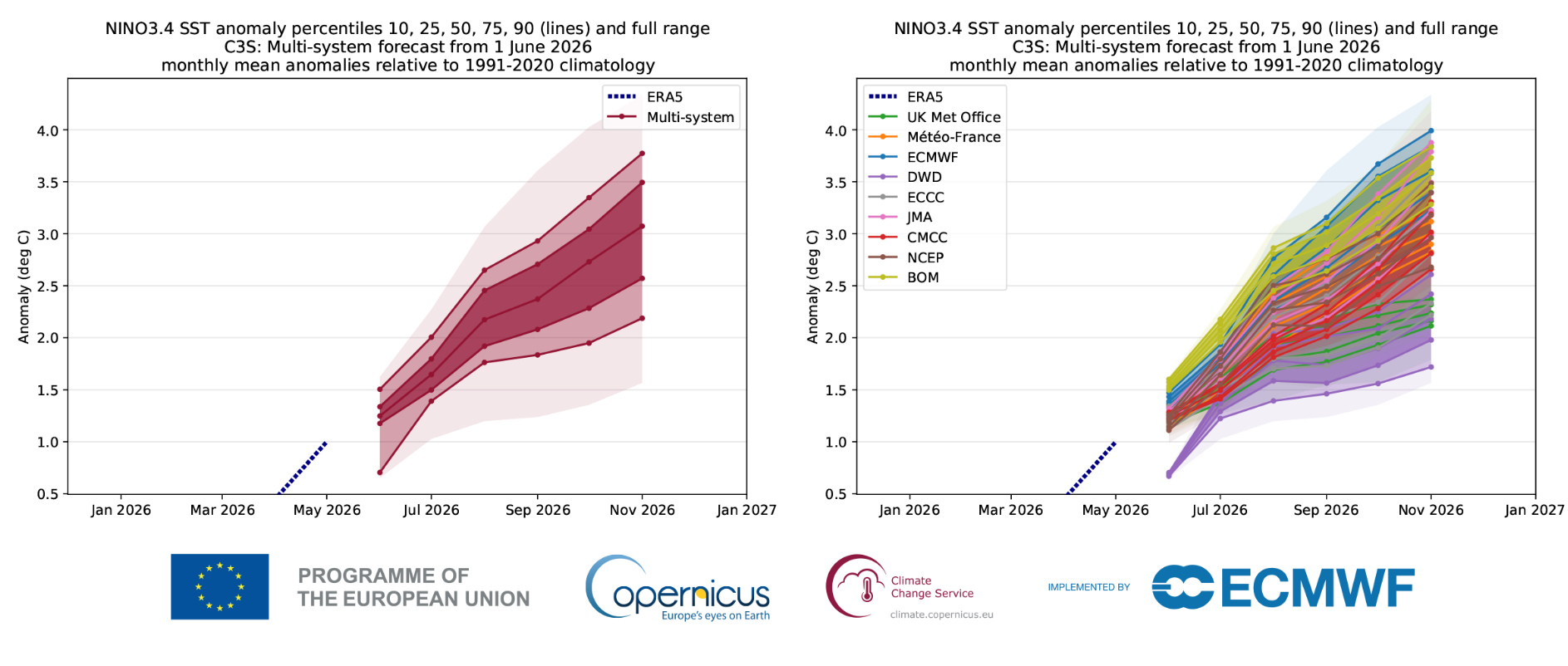
Fig. 4.6.1 The C3S multimodel June 2026 forecast of the of the NINO3.4 index highlighted the likelihood of a large El Nino event developing through the latter part of the year. 75% of members of the grand ensemble exceed 2.5°C amplitude in the Nino3.4 index at the end of the forecast period (November)#
Plume charts of NINO predictions are available on the C3S multi-model SST indices page. Correlation heatmaps for the SST indices from individual models are available here
📋 Methodology#
This notebook provides information on the use of seasonal forecast data available under different C3S catalogues, such as monthly statistics on single levels and and on pressure levels, subdaily data on single levels and on pressure levels, monthly anomalies on single levels and on pressure levels.
The notebook focuses on the review of selected scientific literature on the state-of-the art knowledge and practice in the use of multi-model ensembles.
The discussion is organized in the following sections:
1. Why the multi-model ensemble (MME)
Health
Agriculture
Water resource management
Energy
Disaster preparedness
High-impact events
3. Technical aspects in using the MME approach
Bias adjustment
Combination
📈 Analysis and results#
1. Why the multi-model ensemble (MME)#
There are two main sources of error which affect the performance of seasonal climate predictions in terms of reliability, accuracy and ultimately their usability and value for sectoral applications:
the initial condition uncertainties associated to the knowledge of the current state of the climate system, which is the starting point of a forecast [4];
the errors introduced by climate models, which describe the climate system by means of a finite number - albeit an incredibly large one - of interacting elements and by a set of empirical parametrizations and approximations of physical processes [5].
The first source of error is, to a large extent, unavoidable because it is associated with the limits of the global observing system and to the techniques adopted to extract information from observations. This limit is generally addressed by producing the largest possible ensembles of forecasts with similar initial conditions. The objective of producing large ensembles of forecasts is not necessarily, and only, the elimination or reduction of the forecast uncertainty. Instead, large ensembles aim at providing more robust statistics and produce the largest range of possible outcomes associated with uncertainty of the state of the climate system.
The second source of errors depends on the overall modelling approach, on the parameterizations adopted for some physical processes in the climate system, and on the specific solutions adopted for implementation of each climate modelling system. A fundamental goal of climate modelers is to reduce this kind of error as much as possible, in order to avoid the systematic misrepresentation of key features of the climate system (the so-called model bias), and the associated impact on essential climate variables such as precipitation intensity, temperature, or wind patterns.
The MME approach addresses the second source of error by leveraging the underlying assumption that seasonal predictions produced by different forecasting centers can be considered as the members of a single statistical ensemble. A further assumption is that the systematic errors produced by different climate models can partially compensate each other if the technical choices made for their development are sufficiently independent.
2. Use cases and user needs#
The MME approach to seasonal forecasting has already been tested in a number of applications to demonstrate the advantages over using a single modelling system.
Climate information is designed to meet specific user needs and a one-size-fits-all solution, rather than a systematic collection of existing applications, would be of limited use, if at all possible.
Therefore, a few examples of sectoral applications of the multi-model ensemble approach are provided with the purpose of illustrating real use cases and describe the potential added value of the MME approach.
Health#
An early assessment of the added value of the multi-model approach has been conducted by focusing on malaria early warnings for southern Africa, using the models participating in the DEMETER project which still constitute the core of the C3S multi-model [6] [7]. To generate the MME the difference in means and ratio of variances between each model and a reference dataset is computed and applied to the predictions of the target year. In the DEMETER multi system, the fact that the sub-grid parameterizations in the component models have, to a large extent, been developed independently, is explicitly mentioned as a varied source of model uncertainty associated with the numerical approximation to the underlying partial differential equations that govern climate models.
Agriculture#
At the global scale, two alternative approaches (average method and mosaic method) have been assessed for the forecasting of year-to-year variations in the global yield of key crop commodities such as maize, rice, wheat and soybean. The ROC score analysis of within-season national yield predictions for maize, rice, wheat, and soybean based on mosaic method indicate skillful within-season predictions, especially for maize and wheat [8].
The average method considers a simple average, with equal weights, over multiple forecasting systems for each location and cropping season. Within the mosaic method, the single best-performing forecasting system is selected for each location and cropping season, based on the corresponding grid-based skill score for yield variability. This study uses only one of the models available in C3S (NCEP) along with other SF available from other forecasting centres (APEC Climate Center, Korea; Meteorological Service of Canada; NASA; Pusan National University, Korea). For this application the mosaic method outperforms the average method and, by definition, it also outperforms the performance of individual forecasting systems. However, it may not be suitable for applications requiring large-scale consistency in forecasts, such as hydrological modeling (see below), where maintaining water mass conservation is essential for accurate streamflow predictions. In this case, the simple averaging of multi-model members has been adopted as a more relevant approach [9] .
On a more regional scale, a tailored multi-model ensemble has been developed to forecast national wheat yield in Argentina [10].
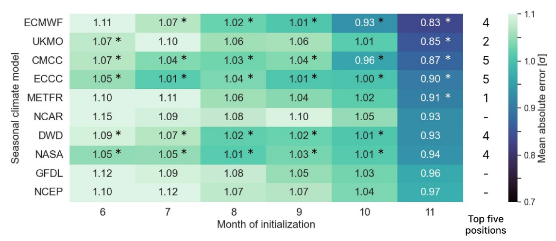
Fig. 4.6.2 Example of mean absolute error between forecasted and reanalysis climate indicators for different forecasting systems and month of initialization. Column-wise for each month of initialization, the mean absolute error is expressed in units of standard deviation (σ), given that all features underwent standardization during preprocessing. Reproduced from [Zachow et al. (2024] under [CC BY 4.0].#
This study considers all but one of the forecasting systems available at C3S and those available through the North-American-Multi-Model Ensemble (NMME). In this case, the multi-model ensemble is built by filtering out the group of three best-performing models for the region and for crop modelling application of interest. Interestingly, out of the initial set of 10 forecasting systems, the final best-performing subset of three systems is a mix of elements coming from both the C3S and of the NMME ensembles.
Water resource management#
C3S has supported the development of an End-to-end Demonstrator for Improved Decision Making in the water sector in Europe (EdgE, [11] ) based on the implementation of a multi-model prediction of streamflow at the European scale. In this case, four different climate modelling systems have been considered, in combination with four different approaches for the computation of the streamflow associated with the seasonal forecasts. This study emphasises how the multi-model approach allows for a better assessment of the uncertainty in the forecast and therefore a better framing of the value of the prediction for decision making.
Energy#
The multi-model seasonal forecast approach has been tested for applications in the energy sector, both for energy production from renewable energy [12] and to forecast energy demand [13] at the national level. It has been demonstrated that:
MME predictions indicate consistently higher performance than individual models in terms of different skill metrics such as temporal correlation coefficient (TCC) [14] and fair ranked probability skill score (FRPSS) [12];
the performance of a multi-model ensemble increases when using climate models which are as independent as possible from each other [13].
Disaster preparedness#
The use of multi-model seasonal forecasts has also emerged as a promising approach to enhance disaster preparedness and management efforts.
For example, advanced flood preparedness in Perù has leveraged multi-model seasonal climate predictions [15] by adopting a mix of best-performing climate model selection and model combination, starting from the North-America Multi-Model Ensemble NMME. The correlation between spring (FMA) precipitation and streamflow (the key impact indicator for this use case) is around 0.76 for individual models whereas it increases to 0.84 when averaging the outcome of the best-performing models from NMME.
A multi-model ensemble composed of 7 out of the 13 systems included in the NMME has been calibrated to enhance climate services in Ethiopia [16], whose National Meteorological Agency is particularly focused on issuing drought early warnings and supporting disaster preparedness and management. In this case, the multi-model ensemble is built by first correcting the bias in each model (i.e. calibration) and then creating a super-ensemble where each model is assigned the same weight independently of the predictive skill.
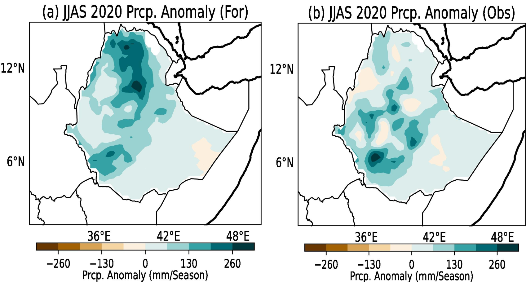
Fig. 4.6.3 JJAS (Kiremt rainy season) precipitation anomalies in Ethiopia for 2020 (a) forecasted (b) observed. Unit of precipitation anomaly is mm/season. Reproduced from Acharya et al. (2021) under CC BY-NC-ND 4.0.#
The analysis of the added value of the multi-model prediction compared to individual models is not explicitly reported. However the study emphasises the main source of predictability in the region is ENSO, whose prediction is known to benefit significantly from the multi-model approach [17].
High-impact events#
The prediction of tropical storm frequency also benefits from the adoption of the multi-model approach as demonstrated using seven models participating in the DEMETER project [18]. By adding all ensemble forecasts after calibration, this analysis demonstrates that over specific regions, combining several models leads to better forecasts than the best individual model.
The analysis conducted during the ENSEMBLES project has demonstrated that the skill in forecasting different indices for temperature and rainfall extremes improves with a multi-model approach, compared to any individual model [19]. This study makes limited, if any, reference to the added value for specific sectoral applications.
Also, the most significant improvements are mainly detected over the tropical ocean in the ENSO region. However, the study provides a key support for the development of applications that rely on the extracting information from the teleconnection between ENSO and local climate variables [17].
3. Technical aspects in using the MME approach#
The MME approach is designed to address multiple sources of climate model uncertainty, including not only differences in the numerical approximations to the governing physical equations, but also variations arising from ensemble size, sampling of initial condition uncertainty, data assimilation techniques, and other aspects of the modeling systems. By combining outputs from multiple models, the MME approach aims to provide more robust and reliable projections than single models alone.
Two main groups of post-processing approaches are adopted to implement the MME approach:
the bias adjustment and recalibration methods applied to the output of individual forecasting systems [20];
the combination of predictions issued with different forecasting systems [21] [22].
Bias adjustment#
Bias adjustment and recalibration methods have been tested systematically on the datasets available on the Copernicus Data Store [21].
On the other hand, the multi-model approach based on combining predictions from different systems assumes that climate models are sufficiently independent to improve or at least partially compensate for the respective errors.
It has been demonstrated, using both toy-models and actual climate model simulations, that multi-model ensembles can outperform a ‘best-model’ approach because multi-model combinations reduce the average ensemble mean error at the cost of widening the spread of the overall ensemble [23].
A systematic, effective approach for the creation of multimodel ensemble, tested on C3S includes, recalibration and the equally weighting of all members of the multi-model ensemble [24].
Combination#
In general, the multi-model approach is expected to bring much of its added value in the tropics, where the combination of models in a single grand-ensemble can offset errors affecting the predictable components of the climate system [25].
In extratropical regions, e.g. over Europe, the multi-model does not always perform better than the best single models, therefore it is advisable to test the single models for each application [26]. The figure below shows an example of how different models can be more skillful over different areas.
Seasonal forecasting studies employ different approaches to generate multi‐model ensembles. As examples:
Complementarity of bias adjustment and combination#
While bias correction and model combination are sometimes discussed separately, they are in fact complementary components of the multi-model ensemble framework rather than competing alternatives. Bias correction improves the performance of individual models, ensuring that each contributes more reliable information to the ensemble. Model combination, in turn, integrates the corrected forecasts from multiple systems to capture a broader range of plausible outcomes and reduce the influence of any single model’s systematic deficiencies.
This complementarity between bias correction and model combination is also supported by comparison of the predictive skill of individual seasonal forecasting systems, which varies substantially across regions, variables, and seasons, with different models achieving the highest anomaly correlation in different areas [26]. Such results highlight that no single forecasting system consistently outperforms all others. Consequently, combining forecasts from multiple models provides an opportunity to exploit the strengths of each system while mitigating their individual weaknesses. Within this framework, bias correction enhances the reliability of the forecasts produced by each model, whereas model combination synthesizes the corrected predictions to generate a more robust and skillful ensemble forecast. Together, these approaches may contribute to improving both forecast calibration and predictive performance.
The Signal to Noise Paradox#
The systematic analysis of climate forecasts has revealed the existence of the so-called Signal-to-Noise Paradox (SNP). This paradox refers to the unexpected situation in which seasonal forecast models can predict the observed climate anomalies more accurately than they can predict their own internal variability.
For example, in winter NAO forecasts, the ensemble mean can anticipate whether the season will be dominated by a positive or negative NAO phase (i.e. stronger or weaker westerly winds over the North Atlantic) even though the individual ensemble members within the same model vary so much from each other that, taken separately, they appear to have very little predictive power. The mismatch between good prediction of reality despite weak internal consistency defines the Signal-to-Noise Paradox. [29]
This is paradoxical because, in principle, if the model is realistic, the predictability within the model’s ensemble should be similar to that of the real world. The existance of a Signal-to-Noise Paradox suggests that the models are underestimating amplitude of their own predictable signal or overestimating internal noise, pointing to systematic deficiencies in the forecasting systems, which are still unclear. [30].
Nonetheless, it has been shown that, in a multi-model ensemble, the signal-to-noise ratio (SNR) can offer valuable insights into forecast reliability. In particular, years characterised by a high SNR tend to exhibit, on average, larger observed deviations from the mean than years with a low SNR, for both near-surface temperature (T2m) and precipitation. This suggests that forecast systems might be more reliable in predicting large anomalies (e.g., extremes) when there is greater coherence among ensemble members [31].
4. The MME approach at work for the C3S multi-model#
On a monthly basis, C3S issues seasonal forecast charts based on the multi-model data available here.
In this case, the seasonal outlook is not designed for specific applications. The multi-model ensemble (MME) forecast is calculated as a weighted average of the ensemble means from nine component models: ECMWF, Met Office, Météo-France, CMCC, DWD, NCEP, JMA, BOM and ECCC.
The weighting ensures that each component contributes equally to the overall variance of the multi-model during the common hindcast period. For each component model, ensemble mean anomalies are calculated relative to its own model climate.
When computing the multi-model mean, the weight assigned to each component is determined by dividing the square root of the average variance across all systems by the square root of the variance of the respective component.
A slightly different approach is adopted for the North American Multi-Model Ensemble (NMME). In this case, to calculate anomalies the forecast bias is removed and is calculated separately for each model using all ensemble members for that particular model. The grand ensemble mean, and other diagnostics such as tercile probabilities, are defined as by assuming assuming that each ensemble member of each model is equally probable .
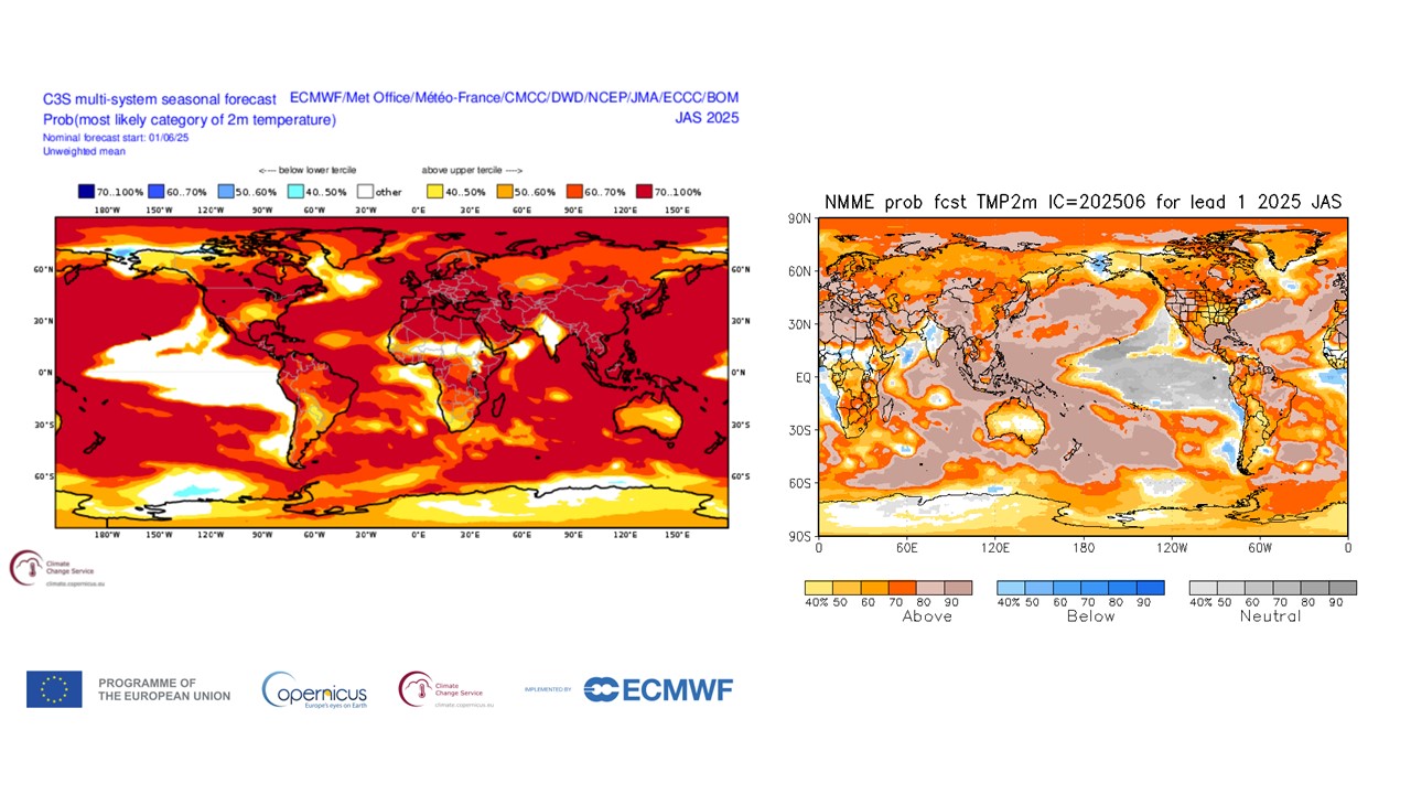
Fig. 4.6.4 Comparison of the July-August-Septmeber 2025 probabilities of above/below/neutral sea surface temperature anomalies forecasted in June 2025, according to the C3S MME (left) and to the NMME (right) methodologies. Note the differences in the respective probabilities as well as the similarities in terms of the overall patterns of global anomalies.#
5. Challenges and Limitations#
The use of a multi-model approach is case specific and there is no evidence of a single standard approach to be adopted as an all-purpose solution.
For example, bias adjustment is essential when preparing the (usually daily based) input for downstream impact models, such as crop models or energy production models. In such circumstances, the added value of a multi-model approach may be off-set by the computational demand of the processing chain. On the other hand, recalibration approaches improve the overall reliability of seasonal indicators by building on the temporal correspondence between the ensemble mean predictions and the corresponding observations [21].
ℹ️ If you want to know more#
Key resources#
Explore the C3S Seasonal Forecast Products
Explore the North American Multi-Model Ensemble products
PyCPT - a tool calibrate and verify multi-model seasonal forecasts of precipitation based on the NOAA North American Multi-Model Ensemble (NMME) and European Copernicus Climate Change Service (C3S) databases.
References#
[1] Hagedorn, R., Doblas-Reyes, F. J., & Palmer, T. N. (2006). DEMETER and the application of seasonal forecasts. Predictability of weather and climate, 674-692.
[2] Vitart, F., Huddleston, M. R., Déqué, M., Peake, D., Palmer, T. N., Stockdale, T. N., … & Weisheimer, A. (2007). Dynamically‐based seasonal forecasts of Atlantic tropical storm activity issued in June by EUROSIP. Geophysical Research Letters, 34(16).
[3] Rajeevan, M., Unnikrishnan, C.K. & Preethi, B. Evaluation of the ENSEMBLES multi-model seasonal forecasts of Indian summer monsoon variability. Clim Dyn 38, 2257–2274 (2012).
[4] Molteni, F., Buizza, R., Palmer, T. N., & Petroliagis, T. (1996). The ECMWF ensemble prediction system: Methodology and validation. Quarterly journal of the royal meteorological society, 122(529), 73-119.
[5] Palmer, T. N. (2001). A nonlinear dynamical perspective on model error: A proposal for non‐local stochastic‐dynamic parametrization in weather and climate prediction models. Quarterly Journal of the Royal Meteorological Society, 127(572), 279-304.
[6] Thomson, M., Doblas-Reyes, F., Mason, S. et al. Malaria early warnings based on seasonal climate forecasts from multi-model ensembles. Nature 439, 576–579
[7] Morse, A. P., Doblas-Reyes, F. J., Hoshen, M. B., Hagedorn, R., & Palmer, T. N. (2005). A forecast quality assessment of an end-to-end probabilistic multi-model seasonal forecast system using a malaria model. Tellus A: Dynamic Meteorology and Oceanography, 57(3), 464–475. https://doi.org/10.3402/tellusa.v57i3.14668
[8] Iizumi, T., Shin, Y., Kim, W., Kim, M., & Choi, J. (2018). Global crop yield forecasting using seasonal climate information from a multi-model ensemble. Climate Services, 11, 13-23.
[9] Thébault, C., Perrin, C., Andréassian, V., Thirel, G., Legrand, S., & Delaigue, O. (2023). Multi-model approach in a variable spatial framework for streamflow simulation. EGUsphere, 2023, 1-34.
[10] , Maximilian Zachow, Harald Kunstmann, Daniel Julio Miralles and Senthold Asseng (2024) Multi-model ensembles for regional and national wheat yield forecasts in Argentina Environ. Res. Lett. 19 084037
[11]Wanders, N., S. Thober, R. Kumar, M. Pan, J. Sheffield, L. Samaniego, and E. F. Wood, 2019: Development and Evaluation of a Pan-European Multimodel Seasonal Hydrological Forecasting System. J. Hydrometeor., 20, 99–115, https://doi.org/10.1175/JHM-D-18-0040.1 .
[12] Lee, D. Y., Doblas-Reyes, F. J., Torralba, V., & Gonzalez-Reviriego, N. (2019). Multi-model seasonal forecasts for the wind energy sector. Climate Dynamics, 53, 2715-2729.
[13] Alessandri, A., Felice, M.D., Catalano, F. et al. Grand European and Asian-Pacific multi-model seasonal forecasts: maximization of skill and of potential economical value to end-users . Clim Dyn 50, 2719–2738 (2018).
[14] Mendoza, P. A., Rajagopalan, B., Clark, M. P., Cortés, G., & McPhee, J. (2014). A robust multimodel framework for ensemble seasonal hydroclimatic forecasts. Water Resources Research, 50(7), 6030-6052.
[15] Keating, C., Lee, D., Bazo, J., and Block, P.: Leveraging multi-model season-ahead streamflow forecasts to trigger advanced flood preparedness in Peru, Nat. Hazards Earth Syst. Sci., 21, 2215–2231,
[16] N. Acharya, M.A. Ehsan, A. Admasu, A. Teshome, K.J.C. Hall (2021) On the next generation (NextGen) seasonal prediction system to enhance climate services over Ethiopia Clim. Serv., 24 (2021), 10.1016/j.cliser.2021.100272
[17] Tippett, M. K., & Barnston, A. G. (2008). Skill of multimodel ENSO probability forecasts. Monthly Weather Review, 136(10), 3933-3946.
[18] Vitart, F. (2006), Seasonal forecasting of tropical storm frequency using a multi-model ensemble. Q.J.R. Meteorol. Soc., 132: 647-666. https://doi.org/10.1256/qj.05.65
[19] Acacia S. Pepler, Leandro B. Díaz, Chloé Prodhomme, Francisco J. Doblas-Reyes, Arun Kumar, The ability of a multi-model seasonal forecasting ensemble to forecast the frequency of warm, cold and wet extremes (2015) , Weather and Climate Extremes, https://doi.org/10.1016/j.wace.2015.06.005 .
[20] Manzanas, R., Gutiérrez, J.M., Bhend, J. et al. Bias adjustment and ensemble recalibration methods for seasonal forecasting: a comprehensive intercomparison using the C3S dataset. Clim Dyn 53, 1287–1305 (2019). https://doi.org/10.1007/s00382-019-04640-4
[21] Krishnamurti, T. N., Kishtawal, C. M., LaRow, T. E., Bachiochi, D. R., Zhang, Z., Williford, C. E., … & Surendran, S. (1999). Improved weather and seasonal climate forecasts from multimodel superensemble. Science, 285(5433), 1548-1550.
[22] Hagedorn, R., Doblas-Reyes, F. J., & Palmer, T. N. (2005). The rationale behind the success of multi-model ensembles in seasonal forecasting — I. Basic concept. Tellus A: Dynamic Meteorology and Oceanography, 57(3), 219–233. https://doi.org/10.3402/tellusa.v57i3.14657
[23] Weigel, A. P., Liniger, M. A., & Appenzeller, C. (2008). Can multi‐model combination really enhance the prediction skill of probabilistic ensemble forecasts?. Quarterly Journal of the Royal Meteorological Society: A journal of the atmospheric sciences, applied meteorology and physical oceanography, 134(630), 241-260.
[24] Hemri, S., Bhend, J., Liniger, M.A. et al. How to create an operational multi-model of seasonal forecasts?. Clim Dyn 55, 1141–1157 (2020). https://doi.org/10.1007/s00382-020-05314-2
[25] Doblas-Reyes, F. J., Hagedorn, R., & Palmer, T. N. (2005). The rationale behind the success of multi-model ensembles in seasonal forecasting – II. Calibration and combination. Tellus A: Dynamic Meteorology and Oceanography, 57(3), 234–252.
[26] Mishra N, Prodhomme C, Guemas V (2018) Multi-model skill assessment of seasonal temperature and precipitation forecasts over Europe. Clim Dyn.
[27] Robertson, A. W., Lall, U., Zebiak, S. E., & Goddard, L. (2004). Improved combination of multiple atmospheric GCM ensembles for seasonal prediction. Monthly Weather Review, 132(12), 2732-2744.
[28] Barnston, A. G., Mason, S. J., Goddard, L., DeWitt, D. G., & Zebiak, S. E. (2003). Multimodel ensembling in seasonal climate forecasting at IRI. Bulletin of the American Meteorological Society, 84(12), 1783-1796.
[29] Scaife, A. A., & Smith, D. (2018). A signal-to-noise paradox in climate science. npj Climate and Atmospheric Science, 1(1), 28.
[30] Weisheimer, A., Baker, L. H., Bröcker, J., Garfinkel, C. I., Hardiman, S. C., Hodson, D. L., … & Sutton, R. T. (2024). The signal-to-noise paradox in climate forecasts: revisiting our understanding and identifying future priorities. Bulletin of the American Meteorological Society, 105(3), E651-E659.
[31] Acosta Navarro, J. C., & Toreti, A. (2023). Exploiting the signal-to-noise ratio in multi-system predictions of boreal summer precipitation and temperature. Weather and Climate Dynamics, 4(3), 823-831.