

1.6.6. Long-term global Eddy Kinetic Energy trends from satellite observations#
Production date: 4-11-2025
Produced by: Joan Armajach and Blanca Fernández-Álvarez - IMEDEA (CSIC-UIB) [webpage]
🌍 Use case: Evaluation of long-term Eddy Kinetic Energy trends#
❓ Quality assessment questions#
Can we assess the long-term variability of global ocean Eddy Kinetic Energy using satellite altimetry?
Global ocean circulation is both a cause and consequence of fluid interactions occurring across a wide range of spatial scales, from millimetres to more than 10,000 km [1]. For ocean circulation, most of the available energy is expressed as kinetic energy (KE), which is a suitable index for measuring the intensity of ocean currents [2]. Mesoscale variability, which ranges from tens to hundreds of kilometers depending on latitude [3], contains nearly all of the ocean’s KE and represents the dominant signal in ocean circulation [4]. About 90% of the total KE is associated with the mesoscale activity, called Eddy Kinetic Energy (EKE) [1, 5]. Meanders, eddies, fronts and jets are examples of mesoscale features that contribute a large part of the transport of heat, mass and chemical constituents in seawater [6]. Consequently, the dynamics of mesoscale features has a notable impact on the surface circulation and oceanic biogeochemistry, spanning local and global scales [7]. To study the evolution of the EKE, gridded satellite sea level anomaly (SLA) products are widely used [8]. Over the last two decades, satellite altimetry has significantly improved our ability to observe and understand ocean circulation at the mesoscale, providing global, high-resolution, and regular monitoring capabilities [9, 10]. At present, over 30 years of altimetric EKE time series are available, and several studies have reported a strengthening trend per decade in some energetic regions (e.g., [5, 11, 12]). In long-term studies from satellite observations, we need to consider that gridded energy levels can vary depending on the data processing and the number of the altimeter missions [13]. As highlighted in [13], a consistent sampling over time from the 2-satellite configuration is recommended for the evaluation of long-term EKE.
This notebook aims to assess the performance of sea level data from satellite observations to estimate the global EKE trends over 1993-2022, following Barceló-Llull et al. (2025).
📢 Quality assessment statement#
These are the key outcomes of this assessment
At the global level, mesoscale activity has intensified over the last decade. Most of this strengthening is consistently concentrated in regions characterized by high Eddy Kinetic Energy (EKE) in both the vDT2021 and vDT2024 datasets.
When comparing the sea level products distributed through the Climate Data Store (CDS), the vDT2021 dataset produces higher EKE both in the global ocean and in high-EKE regions throughout the studied period. Nevertheless, in regions such as the Kuroshio Extension (KExt), these differences between versions are much smaller. This demonstrates that a two-satellite constellation can properly capture mesoscale activity. A constellation with a stable number of satellites ensures the long-term stability of the data record, as is the case for this product, making it a suitable tool for this type of study.
In general, we recommend using the vDT2024 version, as it incorporates new input L2P (Level-2 Plus) altimeter standards compared to the older version (vDT2021). The L2P products serve as the main input for the altimeter-derived sea level production system, providing the necessary information to compute the along-track Sea Level Anomalies (SLA), while applying the same updated corrections and models for the altimeter missions.
📋 Methodology#
Satellite Altimerty based sea level datasets are distributed by the Copernicus Marine Environment Monitoring Service (CMEMS) and the Copernicus Climate Change Service (C3S). In this assessment, we use the Sea level gridded data from satellite observations provided by the CDS. This product is designed for climate applications and is based on a consistent and stable altimeter constellation to ensure the long-term stability of the ocean observing system. The constellation of the C3S product comprises more than 10 satellites, configured to ensure that two altimeters are always active. Of the satellites, one is always the active reference altimetry mission. Although there are changes over time, each replacement mission follows the same orbit, ensuring consistency. The other, known as the secondary mission, is a complementary satellite that provides significant information for estimating mesoscale signals. All the necessary information can be found in the Product User Guide and Specification (PUGS).
As previously mentioned, we follow the same methodology as in [5] to estimate EKE time series and trends over the global ocean. In addition, we quantify EKE in regions of high mesoscale activity, as performed in that study. The authors used the vDT2018 and vDT2021 two-satellite products from C3S to compare them with the vDT2021 all-satellite product provided by CMEMS. The latter uses all available satellites, ranging from 2 to 7 over the altimetric period.
In this study, the vDT2024 version of the satellite gridded sea level observations available in the Climate Data Store is compared with the vDT2021, in order to evaluate how the new version resolves the EKE relative to the previous one. The TOPEX-A instrument drift correction for 1993-1998, which has been quantified in many studies (e.g., [14]), has not yet been computed in the vDT2024 data. In contrast, the vDT2021 product implements this correction as a separate variable (not directly included in the SLA estimate).
The analysis and results are organised in the following steps, which are detailed in the sections below:
Set up the python environment and import required libraries
Define the startup parameters
Define request for satellite altimetry, using both vDT2021 and vDT2024 datasets available from CDS
2. Eddy Kinetic Energy (EKE) computation
3. Definition of high EKE regions
4. EKE time series and trends computation
5. Plotting and discussion of results
High EKE regions
Area-weighted mean EKE time series
EKE trends
📈 Analysis and results#
1. Data selection and setup#
Import required libraries#
First we import the necessary packages.
Define startup parameters#
For this study, we select the period from 1993 to 2022. Moreover, we apply a mask to include only latitudes between 65°S and 65°N, ensuring that satellite observations remain consistent and are not affected by sea ice.
Define data request for satellite altimetry (vDT2021 and vDT2024)#
Here, we define the data request for the global gridded daily sea level products for each version (vDT2021 and vDT2024) using the CDS API client.
2. Eddy Kinetic Energy (EKE) computation#
To compute EKE, we apply the specific formula:
where \(u_a^2\) and \(v_a^2\) refer to the zonal and meridional components of the geostrophic velocity anomalies, respectively. These variables are derived from the gridded SLA field. The computation is based on a 9-point stencil width [15] for latitudes outside the ±5°N band. In the equatorial band, the Lagerloef method [16] is applied, using the β plane approximation.
In this part, we download the datasets according to the request, integrating the function that computes EKE once all the data are available. Chunks are necessary to manage large volumes of information. Finally, we concatenate the EKE data along the dimension “version”.
3. Definition of high EKE regions#
As described in [5], specific areas with high mesoscale activity due to their ocean dynamics are referred to as high EKE regions. To identify these high-intensity regions, the 90th spatial percentile of the mean EKE over the full period (1993-2022) is computed.
Once we have identified the areas with high EKE activity, we define these regions using the latitude and longitude bounds for each region. These regions are: Brazil-Malvinas Confluence (BMC), Loop Current (LC), Gulf Stream (GS), Great Whirl and Socotra Eddy (GWSE), Agulhas Current (AC), Kuroshio Extension (KExt), and East Australian Current (EAC).
For the regions with high EKE, we apply a function that fills holes, removes small regions using a threshold, and smooths contours. This results in well-defined regions and the minimisation of the spurious inclusion of small patches.
We create a dataset with the masks of all individual high EKE regions, previously defined as “regions”. First, we generate a binary global mask based on the mean EKE, where values of 1 mean that the threshold (90th percentile) is exceeded, and values of 0 represent otherwise. Once done, we extract the high EKE regions and apply the smoothing function. Then, we concatenate all the regional masks along the dimension named “region” to differentiate each one.
Additionally, we integrate new masks, one composed of all high EKE regions combined (named “high EKE”), another representing the global mask without NaN values of EKE (named “no ice”), and finally a mask representing the tropical band (named “tropical”), excluding the regions that are already included in “high EKE” mask.
4. EKE time series and trends computation#
In this section, we calculate the area-weighted mean for the spatial averages using latitude weighting. This process is applied to all the masks.
Here, we define the regions used in the test (no ice, high EKE, KExt, and GS) and the dictionaries to store the original time series and a 12-month rolling mean over a continuous period to smooth fluctuations in the data.
For the computation of EKE trends, we implement the Theil-Sen estimator, a non-parametric method for fitting a line to sample points. This regression algorithm is more robust to outliers compared to ordinary least-squares regression, which is sensitive to them. To assess the significance of trends, we use the Mann-Kendall test. However, the presence of serial correlation in time series can affect the results [17]. Therefore, we employ the modified Mann-Kendall test proposed by [17], which accounts for this autocorrelation.
Furthermore, we convert the trends, initially in cm² s⁻² month⁻¹ to cm² s⁻² year⁻¹ using a factor to facilitate the comparison of the results.
In this case, we calculate the trends over different periods of the EKE time series, starting each trend in a different year between 1993 and 2013 (inclusive) and ending in the last year of the study (2022). The MK test is applied to each EKE time series for every region and version. As before, we create new dictionaries to store all trends and p-values.
5. Plotting and discussion of results#
Before plotting and describing the results, we define a couple of functions to customise the graphs, including both their structure and style.
High EKE regions#
Here, we prepare the high EKE and tropical masks as binary masks for proper visualisation. For the tropical mask, we apply “add_cyclic_point” to avoid discontinuity at 180° longitude. We also exclude these masks when graphing to represent only the individual high EKE regions.
Once the masks have been treated, we display the corresponding graphs in a layout of two subplots.
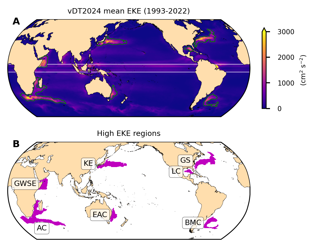
This figure shows a global map of the temporal mean EKE at each grid point over 1993-2022, using only the vDT2024 dataset. The green contours delimit the regions with high EKE activity (over the 90th percentile), and the blue line marks the tropical band. These areas contain most of the mesoscale activity, which averages zero in the remainder part of the globe.
In the other global map, we represent the exact high EKE regions (covering 5% of the global ocean) along with their corresponding acronyms. As a first observation, the largest regions (in terms of area) with high mesoscale activity occur in AC, KExt, and GS. In contrast, LC and EAC are the smallest regions.
Area-weighted mean EKE time series#
In this section, we plot the EKE time series (in cm² s⁻²) over the global ocean and the high EKE regions, including the Kuroshio Extension and the Gulf Stream, covering the altimeter period 1993 to 2022.
Global region#
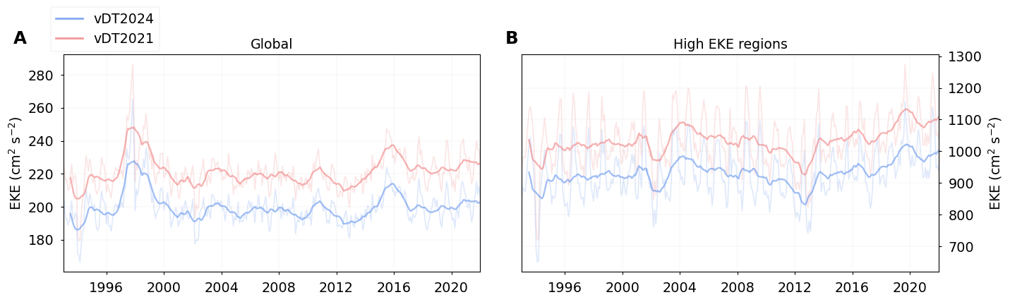
The two subplots show the evolution of EKE in the global and high EKE regions. The color blue represents the vDT2024 version and the color red the vDT2021 version. The thinner lines show the raw (untreated) data, whilst the thicker lines indicate the data after applying an annual rolling mean. Regarding the results, notable differences are observed when comparing the two versions. For both the global ocean and high EKE regions, vDT2021 exhibits higher values throughout the entire period than vDT2024. One possible reason is the methodology used in producing each version, including the metrics, procedures, and equations implemented, resulting in more accurate data in the current version (vDT2024), as mentioned in the Algorithm Theoretical Basis Document. For the global region, the rolling mean values are around 190-250 cm² s⁻² approximately. However, focusing on the high EKE regions, the values increase markedly, reaching up to 1150 cm² s⁻². These regions, as observed, demonstrate high mesoscale activity.
Mesoscale High-Activity Regions#
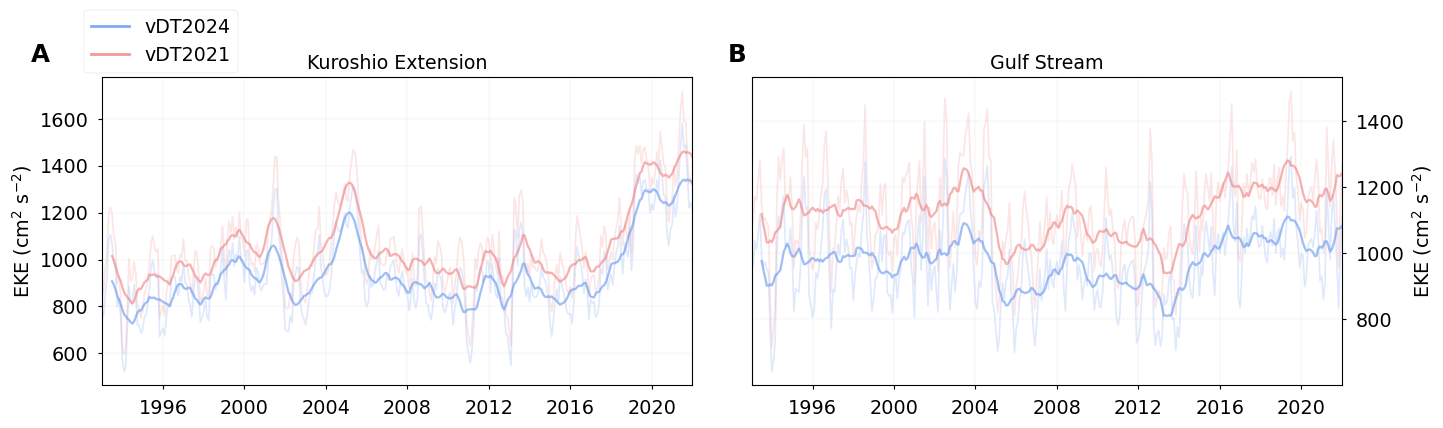
Following [5], two specific areas were selected and compared: the KExt and the GS. Similarly to the previous plot, we have two timeseries for each version (red for the vDT2021 and blue for the vDT2024), with the older version showing higher energy than the newer one. The difference is larger in the GS than in the KExt. When we compare the energy in both areas, both versions point towards an increase in EKE in the KExt. Both versions also capture the variability in the timeseries, with higher seasonal variability in the GS.
EKE trends#
For these plots, we first defined a specific marker and text style to distinguish non-significant trends in the bar plots. Non-significant trends are shown in italics, with oblique grey hatching.
Global region#
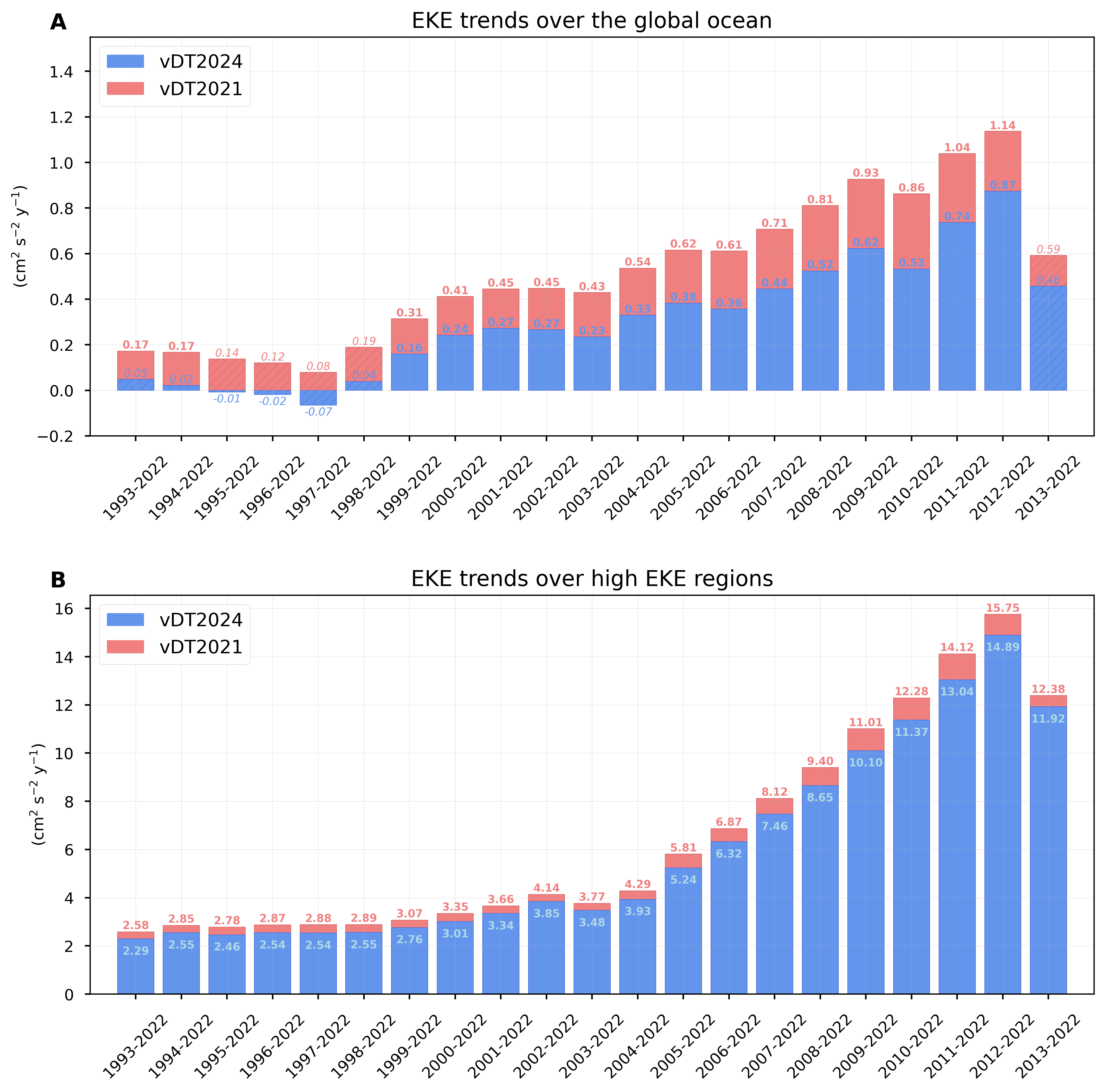
In this case, we can observe the EKE trends over different periods, progressively shortening the intervals to study the trends. For the global ocean, the trends are larger over shorter timescales, reaching a maximum trend of 0.87 cm² s⁻² year⁻¹ (vDT2024) and 1.14 cm² s⁻² year⁻¹ (vDT2021) from 2012 to 2022. Looking in more detail, the initial trends computed with a starting year prior to 2000 show a slight decrease, resulting in non-significant trends for both datasets and even negative trends in the case of vDT2024, for which, if we consider the whole period, the EKE trend is not significant (whereas it is for vDT2021). This behaviour changes drastically after 2000, with a constant increase, revealing an intensification of the mesoscale activity globally.
For the high EKE regions, we can clearly see a substantial increase throughout the full period for both datasets. In this case, all trends are significant, although vDT2021 displays larger values than vDT2024. For the older version, the trend over 2012-2022 is 6.1 times larger than the trend during 1993-2022, increasing from 2.58 cm² s⁻² year⁻¹ to 15.75 cm² s⁻² year⁻¹. However, for the latest version, the trend is 6.5 times larger, from 2.29 cm² s⁻² year⁻¹ to 14.89 cm² s⁻² year⁻¹. This suggests that over the last two decades, EKE activity has become stronger and more energetic, especially in the high EKE regions, with a particularly high rate of increase in the most recent periods.
In [5], the vDT2021 all-sat product from CMEMS is used to compare with the vDT2021 two-sat product from C3S. That study suggests that differences in trends between the two products are partly related to the number of satellites included in the all-sat product.
Mesoscale High-Activity Regions#
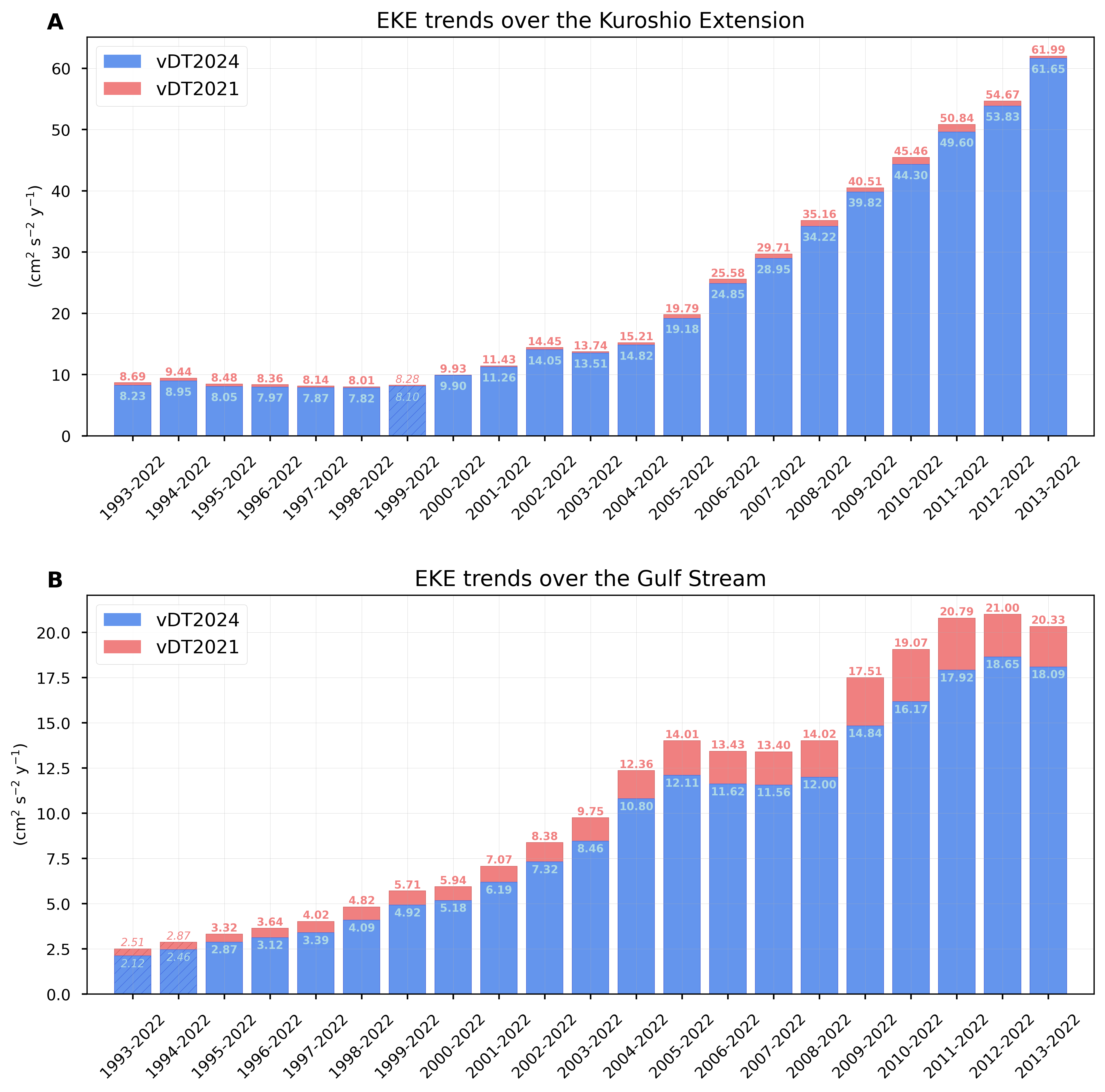
Here, we focus on the regions where the mesoscale activity exhibits more significant positive EKE trends. This intensification is concentrated mainly in the Kuroshio Extension (KExt) and the Gulf Stream (GS). Regarding the KExt region, the computed trends show a progressive increase for both datasets. The vDT2021 presents higher values than vDT2024, but these differences are small compared with the other regions. Only the trend over 1999-2022 is not statistically significant for either version. As mentioned before, this fast increase occurs primarily in the last decade. For the period 2013-2022, the EKE trend for vDT2024 is 61.65 cm² s⁻² year⁻¹ and for vDT2021 is 61.99 cm² s⁻² year⁻¹, while over the entire 30-year period the trends are 8.23 cm² s⁻² year⁻¹ and 8.69 cm² s⁻² year⁻¹, respectively. This region is crucial for ocean circulation and mid-latitudes air-sea interactions and is one of the major western boundary currents [18]. As reported by [19], the decadal variability of EKE in this region is linked to the Pacific Decadal Oscillation (PDO).
In the Gulf Stream (GS), the general trend shows a gradual increase. Over the 30 years, the EKE trends are 2.12 cm² s⁻² year⁻¹ for vDT2024 and 2.51 cm² s⁻² year⁻¹ for vDT2021, both of which are statistically non-significant. In the most recent decade, the trends have increased notably, reaching 18.09 cm² s⁻² year⁻¹ and 20.33 cm² s⁻² year⁻¹, respectively. This corresponds to an increase in the EKE trend of 8.5 and 8.1 times faster than over the entire 30-year period. The GS plays an important role due to its contribution to the Atlantic Meridional Overturning Circulation (AMOC) [20]. [21] reported that the path of the GS is associated with the strength of the AMOC.
ℹ️ If you want to know more#
Key resources#
[5] Barceló-Llull, B., Rosselló, P., Combes, V., Sánchez-Román, A., Pujol, M. I., and Pascual, A. (2025). Kuroshio Extension and Gulf Stream dominate the Eddy Kinetic Energy intensification observed in the global ocean. Scientific Reports, 15(1), 21754. doi: 10.1038/s41598-025-06149-9
CDS entry: Sea level gridded data from satellite observations for the global ocean from 1993 to present.
All the documentation for each version is available here.
Further information:
C3S EQC custom functions,
c3s_eqc_automatic_quality_control, prepared by B-Open.
References#
[1] Ferrari, R., & Wunsch, C. (2009). Ocean circulation kinetic energy: Reservoirs, sources, and sinks. Annual Review of Fluid Mechanics, 41(1), 253-282. doi: 10.1146/annurev.fluid.40.111406.102139
[2] Hu, S., Sprintall, J., Guan, C., McPhaden, M. J., Wang, F., Hu, D., & Cai, W. (2020). Deep-reaching acceleration of global mean ocean circulation over the past two decades. Science advances, 6(6), eaax7727. doi: 10.1126/sciadv.aax7727
[3] Chelton, D. B., DeSzoeke, R. A., Schlax, M. G., El Naggar, K., & Siwertz, N. (1998). Geographical variability of the first baroclinic Rossby radius of deformation. Journal of Physical Oceanography, 28(3), 433-460. doi: 10.1175/1520-0485(1998)028<0433:GVOTFB>2.0.CO;2
[4] Pascual, A., Faugère, Y., Larnicol, G., & Le Traon, P. Y. (2006). Improved description of the ocean mesoscale variability by combining four satellite altimeters. Geophysical Research Letters, 33(2). doi: 10.1029/2005GL024633
[5] Barceló-Llull, B., Rosselló, P., Combes, V., Sánchez-Román, A., Pujol, M. I., & Pascual, A. (2025). Kuroshio Extension and Gulf Stream dominate the Eddy Kinetic Energy intensification observed in the global ocean. Scientific Reports, 15(1), 21754. doi: 10.1038/s41598-025-06149-9
[6] Chelton, D. B., Schlax, M. G., Samelson, R. M., & de Szoeke, R. A. (2007). Global observations of large oceanic eddies. Geophysical Research Letters, 34(15). doi: 10.1029/2007GL030812
[7] Le Vu, B., Stegner, A., & Arsouze, T. (2018). Angular momentum eddy detection and tracking algorithm (AMEDA) and its application to coastal eddy formation. Journal of Atmospheric and Oceanic Technology, 35(4), 739-762. doi: 10.1175/JTECH-D-17-0010.1
[8] Amores, A., Jordà, G., & Monserrat, S. (2019). Ocean eddies in the Mediterranean Sea from satellite altimetry: Sensitivity to satellite track location. Frontiers in Marine Science, 6, 703. doi: 10.3389/fmars.2019.00703
[9] Abdalla, S., Kolahchi, A. A., Ablain, M., Adusumilli, S., Bhowmick, S. A., Alou-Font, E., … & Hamon, M. (2021). Altimetry for the future: Building on 25 years of progress. Advances in Space Research, 68(2), 319-363. doi: 10.1016/j.asr.2021.01.022
[10] Morrow, R., & Le Traon, P. Y. (2012). Recent advances in observing mesoscale ocean dynamics with satellite altimetry. Advances in Space Research, 50(8), 1062-1076. doi: 10.1016/j.asr.2011.09.033
[11] Hargous, P., Combes, V., Barceló-Llull, B., & Pascual, A. (2025). Eddy Kinetic Energy Variability From 30 Years of Altimetry in the Mediterranean Sea. EGUsphere, 2025, 1-22. doi: 10.5194/egusphere-2025-4651
[12] Martínez-Moreno, J., Hogg, A. M., England, M. H., Constantinou, N. C., Kiss, A. E., & Morrison, A. K. (2021). Global changes in oceanic mesoscale currents over the satellite altimetry record. Nature Climate Change, 11(5), 397-403. doi: 10.1038/s41558-021-01006-9
[13] Morrow, R., Fu, L. L., Rio, M. H., Ray, R., Prandi, P., Le Traon, P. Y., & Benveniste, J. (2023). Ocean circulation from space. Surveys in Geophysics, 44(5), 1243-1286. doi: 10.1007/s10712-023-09778-9
[14] Watson, C. S., White, N. J., Church, J. A., King, M. A., Burgette, R. J., & Legresy, B. (2015). Unabated global mean sea-level rise over the satellite altimeter era. Nature Climate Change, 5(6), 565-568. doi: 10.1038/NCLIMATE2635
[15] Arbic, B. K., Scott, R. B., Chelton, D. B., Richman, J. G., & Shriver, J. F. (2012). Effects of stencil width on surface ocean geostrophic velocity and vorticity estimation from gridded satellite altimeter data. Journal of Geophysical Research: Oceans, 117(C3). doi: 10.1029/2011JC007367
[16] Lagerloef, G. S., Mitchum, G. T., Lukas, R. B., & Niiler, P. P. (1999). Tropical Pacific near‐surface currents estimated from altimeter, wind, and drifter data. Journal of Geophysical Research: Oceans, 104(C10), 23313-23326. doi: 10.1029/1999JC900197
[17] Yue, S., & Wang, C. (2004). The Mann-Kendall test modified by effective sample size to detect trend in serially correlated hydrological series. Water resources management, 18(3), 201-218. doi: 10.1023/B:WARM.0000043140.61082.60
[18] Xiaodong, M., Lei, Z., Weishuai, X., Qinghong, L., & Maolin, L. (2024). Analysis and prediction of mesoscale eddy kinetic energy variations in the Kuroshio extension. Dynamics of Atmospheres and Oceans, 108, 101497. doi: 10.1016/j.dynatmoce.2024.101497
[19] Yang, C., Yang, H., Chen, Z., Gan, B., Liu, Y., & Wu, L. (2023). Seasonal variability of eddy characteristics and energetics in the Kuroshio Extension. Ocean Dynamics, 73(8), 531-544. doi: 10.1007/s10236-023-01565-9
[20] Buckley, M. W., & Marshall, J. (2016). Observations, inferences, and mechanisms of the Atlantic Meridional Overturning Circulation: A review. Reviews of Geophysics, 54(1), 5-63. doi: 10.1002/2015RG000493
[21] Joyce, T. M., & Zhang, R. (2010). On the path of the Gulf Stream and the Atlantic meridional overturning circulation. Journal of Climate, 23(11), 3146-3154. doi: 10.1175/2010JCLI3310.1