Sea ice drift from satellite observations: resolution and uncertainty of Arctic sea ice drift for large-scale sea ice transport analysis

1.3.11. Sea ice drift from satellite observations: resolution and uncertainty of Arctic sea ice drift for large-scale sea ice transport analysis#

Production date: 30-04-2026

Dataset version: 1.0

Produced by: Yoni Verhaegen and Philippe Huybrechts (Vrije Universiteit Brussel)

🌍 Use case: Quantifying sea ice transport out of the Arctic Ocean through Fram Strait#

❓ Quality assessment question#

“Is the C3S sea ice drift dataset sufficiently adequate in terms of its spatio-temporal resolution, extent and uncertainty to quantify sea ice volume fluxes through Fram Strait?”

Sea ice drift derived from satellite observations is a fundamental parameter for monitoring changes in polar sea ice dynamics and understanding the impact of climate variability on the Arctic and Antarctic regions. Coinciding with the Arctic warming ratio, which is about 4 times the global average, Arctic sea ice is in decline. In this context, the ‘Sea ice drift daily gridded data derived from satellite observations’ on the Climate Data Store (CDS), provided by the Ocean and Sea Ice Satellite Application Facility (OSI SAF), offers daily sea ice drift vectors and their associated uncertainties for both hemispheres on a 75 km equal area projection grid. They can be interpreted as sea ice motion: the displacement of sea ice within a certain time period [1].

The Fram Strait, situated between Greenland and Svalbard, is the principal gateway through which sea ice exits the Arctic Ocean into the North Atlantic. It is widely recognized as the dominant pathway of freshwater export from the Arctic: approximately 90% of the total sea ice outflow occurs through this strait. On average, the annual Fram Strait export corresponds to roughly 10-15% of the total Arctic sea ice mass [2, 3]. It therefore has a central role in the sea ice mass balance and in modulating ocean-climate interactions between the central Arctic and the North Atlantic Ocean. In this notebook, we will investigate whether the quality of the C3S sea ice drift data, in terms of its spatial/temporal resolution and uncertainty, is sufficient to accurately determine the sea ice volume export through Fram Strait. More specifically, we will check the compliance of the quality indices with GCOS standards and also compare the calculated sea ice volume export with those from independent data. For that, we use the dataset version 1.0 on the CDS.

🚨 Although this notebook deals with the Arctic sea ice only, sea ice drift data for the Antarctic region are also available.

📢 Quality assessment statements#

These are the key outcomes of this assessment

The C3S sea ice drift product offers year-round daily sea ice drift vectors for both hemispheres on a 75 km equal-area projection grid and also includes pixel-level quality flags, as well as quantitative uncertainty estimates. The uncertainty magnitudes generally meet internationally recommended GCOS standards and the daily temporal resolution of the dataset, as well as the year-round and hemispheric extent, are furthermore excellent for many applications and analyses. However, the 75 km spatial resolution remains relatively coarse with respect to the minimum GCOS requirement of 50 km.
With respect to the use case, the C3S sea ice drift product is found to be highly suitable to derive sea ice volume export fluxes through Fram Strait, provided that (i) the data are supplemented with sea ice thickness and sea ice concentration data that have been regridded and resampled to a common aligned grid, and (ii) the sea ice drift vectors are rotated to obtain drift components that are expressed relative to the orientation of the gate before computing the sea ice volume flux. Due to constraints of the other C3S products and the validation data, the volume fluxes were only calculated for the winter months during the 2010-2020 period. The calculated volume fluxes align well with values from independent data over the overlapping period, and their uncertainty bounds are of a similar magnitude when compared to reported values from silimar datasets in the literature. This adds credibility to the product and supports the quality-richness of the C3S data.

📋 Methodology#

Dataset description#

The C3S OSI SAF product combines data from (1) multiple microwave radiometers using feature-tracking techniques to estimate the displacement of sea ice patterns between consecutive satellite images in the winter season, and (2) model-driven sea ice drift fields using ERA5 10 m wind data and a tuned free-drift model in the summer season. The corresponding displacements are converted into drift vectors representing sea ice motion over the time interval between satellite images. Post-processing involves, amongst others, gap-filling by interpolation. To ensure temporal consistency, data from different sensors are homogenized and merged into a continuous data record covering several decades (1991-2020). The dataset provides the zonal and meridional components of sea ice drift on an equal area projection grid, as well as their uncertainty estimates (provided as 1-sigma errors). Data are delivered in NetCDF format and include additional relevant information such as rejection and quality flags. All data follow a consistent projection with drift values expressed in km per day [1].

To calculate sea ice volume export through Fram Strait, the C3S OSI SAF sea ice drift data are in this notebook combined with C3S sea ice thickness and sea ice concentration estimates. For that, we follow the procedure outlined in Ricker et al. (2018) [2] to calculate sea ice volume export through a defined flux gate. Therefore, all data have to be aligned to a common grid and time period. Based on constraints of the other C3S sea ice data, we choose to only calculate monthly sea ice volume export values for the winter months (October to April) of the 2010-2020 period on a 75 km grid. Later on in the notebook, we also calculate the corresponding uncertainties and compare the calculated sea ice volume export values and their uncertainties with independent CMST (Combined Model and Satellite sea ice Thickness) data from Min et al. (2019) [3].

Structure and (sub)sections#

1. Data preparation and processing

1.1 Import packages
1.2 Define request and download
1.3 Display and inspect data

2. Patterns of sea ice motion and its uncertainty

2.1 Average sea ice drift velocities
2.2 Sea ice drift uncertainty

3. Calculating the winter sea ice volume export through Fram Strait between 2010-2020

3.1 Defining the location of the Fram Strait gate
3.2 Calculating winter sea ice export through the Fram Strait
3.3 Sea ice volume export uncertainty

4. Comparison of Fram Strait volume fluxes with independent data

4.1 Comparison of sea ice volume export with CMST data
4.2 Comparison of sea ice volume export uncertainty with CMST data

5. Short summary and take-home messages

📈 Analysis and results#

1. Data preparation and processing#

1.1 Import packages#

First we load the packages:

1.2 Define request and download#

Then we define the parameters, i.e. for which years the data should be downloaded:

Then we define requests for download from the CDS and download and transform the sea ice data. We regrid and resample the data so the temporal and resolution of all datasets are aligned:

Here, we define a function that resamples all data to a common grid (75 km) and time period (monthly data):

Finally, we download the data and apply the transformation function:

collection_id = 'satellite-sea-ice-drift'

100%|██████████| 11/11 [00:00<00:00, 23.07it/s]

collection_id = 'satellite-sea-ice-thickness'

100%|██████████| 11/11 [00:00<00:00, 13.19it/s]

collection_id = 'satellite-sea-ice-concentration'

100%|██████████| 11/11 [00:00<00:00, 15.67it/s]

Downloading done.

1.3 Display and inspect data#

We can read and inspect the data. Let us print out the data to inspect its structure:

<xarray.Dataset> Size: 70MB
Dimensions:                       (time: 77, yc: 144, xc: 144)
Coordinates:
  * time                          (time) datetime64[ns] 616B 2010-01-01 ... 2...
  * yc                            (yc) float64 1kB 5.362e+03 ... -5.362e+03
  * xc                            (xc) float64 1kB -5.362e+03 ... 5.362e+03
    latitude                      (yc, xc) float32 83kB dask.array<chunksize=(144, 144), meta=np.ndarray>
    longitude                     (yc, xc) float32 83kB dask.array<chunksize=(144, 144), meta=np.ndarray>
Data variables:
    Lambert_Azimuthal_Equal_Area  (time) float64 616B dask.array<chunksize=(7,), meta=np.ndarray>
    t0                            (time, yc, xc) datetime64[ns] 13MB dask.array<chunksize=(7, 144, 144), meta=np.ndarray>
    t1                            (time, yc, xc) datetime64[ns] 13MB dask.array<chunksize=(7, 144, 144), meta=np.ndarray>
    lat1                          (time, yc, xc) float32 6MB dask.array<chunksize=(7, 144, 144), meta=np.ndarray>
    lon1                          (time, yc, xc) float32 6MB dask.array<chunksize=(7, 144, 144), meta=np.ndarray>
    dX                            (time, yc, xc) float32 6MB dask.array<chunksize=(7, 144, 144), meta=np.ndarray>
    dY                            (time, yc, xc) float32 6MB dask.array<chunksize=(7, 144, 144), meta=np.ndarray>
    status_flag                   (time, yc, xc) float64 13MB dask.array<chunksize=(7, 144, 144), meta=np.ndarray>
    uncert_dX_and_dY              (time, yc, xc) float32 6MB dask.array<chunksize=(7, 144, 144), meta=np.ndarray>
Attributes: (12/42)
    title:                     Global Sea Ice Drift Climate Data Record Versi...
    summary:                   This climate data record of sea ice drift vect...
    topiccategory:             Oceans ClimatologyMeteorologyAtmosphere
    keywords:                  GCMDSK:Earth Science > Cryosphere > Sea Ice > ...
    keywords_vocabulary:       GCMDSK:GCMD Science Keywords:https://gcmd.eart...
    geospatial_lat_max:        90.0
    ...                        ...
    tracking_id:               3bb67a09-5c29-4945-8c3b-7e629280aaef
    naming_authority:          int.eumetsat
    Conventions:               CF-1.7,ACDD-1.3
    standard_name_vocabulary:  CF Standard Name Table (Version 78, 21 Septemb...
    product_name:              osi_saf_sea_ice_drift_climate_data_record
    doi:                       10.15770/EUM SAF OSI 0012

Here, the downloaded set of the C3S OSI SAF sea ice drift data provides daily satellite and model-derived sea ice drift vectors \(D\) on a 75 km Lambert Azimuthal Equal Area grid covering the entire Arctic. The subset of the dataset used here spans the winter months only (October-April) during the 2010–2020 period with 77 time steps, as data were aggregated (averaged) from a daily to a monthly basis. Sea ice drift components (dX, dY) are provided in grid coordinates together with corresponding latitude/longitude fields and uncertainty estimates (uncert_dX_and_dY). The total drift speed (and its direction) can be computed as the Euclidean norm of (dX, dY):

\(D = \sqrt{D_x^2 + D_y^2}\)

where \(D_x\) and \(D_y\) are the zonal and meridional components of the sea ice drift (in km/day) respectively, defined within the projected grid. In this case, we also downloaded the sea ice thickness and sea ice concentration fields to use them later in this notebook for calculating the total sea ice volume export through Fram Strait. We regridded and resampled these data into a common spatial (i.e. a 75 km spatial resolution) and temporal (i.e. a monthly temporal resolution) frame so that all data align. A variable status_flag further indicates the quality of the data (see the Product User Guide).

2. Patterns of sea ice motion and its uncertainty#

2.1 Average sea ice drift velocities#

We begin by plotting the sea ice drift vectors averaged between the beginning and end period that we selected for the sea ice drift data (i.e. the winter months between 2010-2020) with a defined plotting function. Let us therefore first define a plotting function that uses the displacement components dX and dY to define a vector field:

Show code cell source

Hide code cell source

def plot_mean_drift_arrows(ds, step=1, suptitle=None, cmap="rainbow", scale=100, vmin=2, vmax=16):

    # Time mean of projected drift components (km/day) 
    dX_mean = ds["dX"].mean(dim="time", skipna=True)
    dY_mean = ds["dY"].mean(dim="time", skipna=True)

    # Subsample in grid space 
    U = dX_mean[::step, ::step].values      # km/day along x
    V = dY_mean[::step, ::step].values      # km/day along y

    # Speed for coloring
    S = np.hypot(U, V)

    # Coordinates in LAEA (m)
    x = ds["xc"][::step].values*1000
    y = ds["yc"][::step].values*1000
    XX, YY = np.meshgrid(x, y)

    # Colormap 
    norm = mcolors.Normalize(vmin=vmin, vmax=vmax)
    cmap_obj = plt.colormaps[cmap]

    # Projection 
    proj = ccrs.LambertAzimuthalEqualArea(central_longitude=0, central_latitude=90)

    fig, ax = plt.subplots(figsize=(7.5,7.5),
                           subplot_kw={"projection": proj})

    # Background land/ocean
    ax.add_feature(cfeature.OCEAN, facecolor="lightblue", zorder=0)
    ax.add_feature(cfeature.LAND, facecolor="0.9", edgecolor="black", zorder=1)
    ax.coastlines(linewidth=0.8, zorder=2)
    ax.gridlines(draw_labels=False, linewidth=0.4, linestyle="--",
                 color="gray", alpha=0.5)
    
    # Extent in lon/lat 
    lon_min, lon_max = -30, 90
    lat_min, lat_max = 72.5, 85

    proj = ccrs.LambertAzimuthalEqualArea(central_longitude=0, central_latitude=90)

    xy_min = proj.transform_point(lon_min, lat_min, src_crs=ccrs.PlateCarree())
    xy_max = proj.transform_point(lon_max, lat_max, src_crs=ccrs.PlateCarree())

    xmin, ymin = xy_min
    xmax, ymax = xy_max
    ax.set_extent([xmin, xmax, ymin, ymax], crs=proj)

    # Quiver
    q = ax.quiver(
        XX, YY, U, V, S,
        transform=proj,        # same CRS as axes
        cmap=cmap_obj,
        norm=norm,
        scale=scale,
        width=0.005,
        headwidth=4,
        headlength=4,
        headaxislength=3,
        zorder=3,
    )

    # Colorbar
    cb = fig.colorbar(q, ax=ax, shrink=0.65, pad=0.04, extend="both")
    cb.set_label("Mean drift speed (km/day)")

    # Add some text
    ax.text(-7.5, 79.5, "Fram Strait", transform=ccrs.PlateCarree(), fontsize=11, bbox=dict(facecolor="white", edgecolor="black", alpha=0.6, pad=2))
    ax.text(-35, 79, "Greenland", transform=ccrs.PlateCarree(), fontsize=11, bbox=dict(facecolor="white", edgecolor="black", alpha=0.6, pad=2))
    ax.text(12, 79, "Svalbard", transform=ccrs.PlateCarree(), fontsize=11, bbox=dict(facecolor="white", edgecolor="black", alpha=0.6, pad=2))

    # Add title
    ax.set_title("Mean sea ice drift vectors (winter 2010-2020)", fontsize=14)
    if suptitle:
        fig.suptitle(suptitle, fontsize=16)

    # Plotting
    plt.tight_layout()
    plt.show()

With this function, let us plot the data:

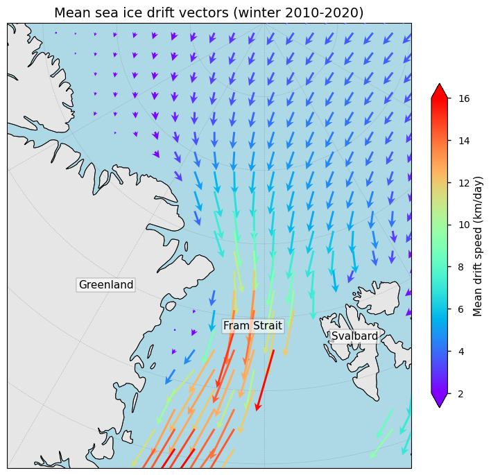
../../_images/d331957d0929d02aa19acfcaf73695334fb8f15c7e01c5fbe8d224b2447f6d77.png

Figure 1. Average sea ice drift vectors across the Fram Strait region (i.e. a subset of the entire domain) during the winter months (October to April) of the 2010-2020 period from the C3S data.

The figure above illustrates the mean winter (October–April) sea ice drift field for 2010–2020, showing the dominant southward export of sea ice through Fram Strait. Drift speeds accelerate markedly as the Transpolar Drift Stream approaches the strait and sea ice gets squeezed in between Greenland and Svalbard. This persistent outflow illustrates Fram Strait’s role as the primary pathway for Arctic sea ice export towards the North Atlantic [2, 3].

2.2 Sea ice drift uncertainty#

Let us now investigate the uncertainties of the sea ice drift data. We begin by plotting a time series of the reported uncertainties within the data uncert_dX_and_dY. The total error of a sea ice drift estimate is theoretically given by both a precision (random) and an accuracy (systematic) error. For the sea ice drift data, the product only deals with precision errors in the form of 1 standard deviation. In this case, the uncertainty can be expressed as \(\sigma_D\).

A time series of the spatially averaged (arithmetic mean) errors reveals the following overall values:

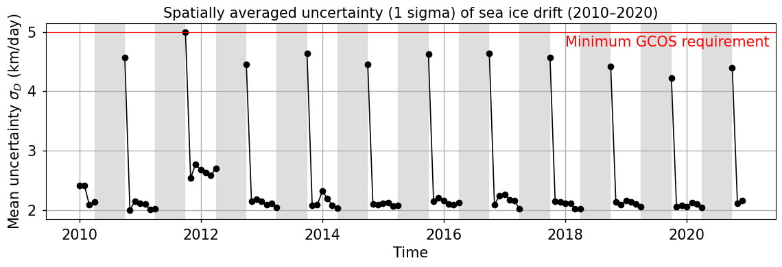
../../_images/26452929a45598e86957a041772da0c9d0f53541f4e92a639d5c4dec88254016.png

Figure 2. Spatially averaged (over the entire Arctic domain) sea ice drift uncertainty (expressed as 1 sigma precision errors) of the winter months (October-April) between 2010-2020 of the C3S data. Shaded intervals indicate the summer months, during which data are not calculated.

The uncertainty assessment shows that overall errors are in the order of 2 to 2.5 km/day for the winter months. Given that the recommended GCOS “threshold” value (i.e. the minimum requirement to be met to ensure that data are useful) is 5 km/day in terms of 1 sigma, the data meet this requirement [5]. However, a characteristic that catches the eye in the above figure is the consistently higher uncertainty for the month October (in the order of 4-5 km/day). This is because the sea ice drift from satellite motion tracking may still be less reliable due to surface melting and increased atmospheric wetness [1]. Let us now calculate the 2D field of these uncertainties:

Show code cell source

Hide code cell source

def plot_mean_field(ds, varname, title=None, cmap=None, vmin=None, vmax=None):

    # Time-mean field 
    da = ds[varname].mean(dim="time", skipna=True)

    # Coordinates (km to m)
    x = ds["xc"].values * 1000
    y = ds["yc"].values * 1000

    # Colormap 
    if vmin is None:
        vmin = float(da.min())
    if vmax is None:
        vmax = float(da.max())

    norm = mcolors.Normalize(vmin=vmin, vmax=vmax)

    # Projection 
    proj = ccrs.LambertAzimuthalEqualArea(central_longitude=0, central_latitude=90)

    fig, ax = plt.subplots(figsize=(8, 8), subplot_kw={"projection": proj})

    # Geographic extent
    lon_min, lon_max = -30, 90
    lat_min, lat_max = 70, 85

    xy_min = proj.transform_point(lon_min, lat_min, src_crs=ccrs.PlateCarree())
    xy_max = proj.transform_point(lon_max, lat_max, src_crs=ccrs.PlateCarree())
    ax.set_extent([xy_min[0], xy_max[0], xy_min[1], xy_max[1]], crs=proj)

    # Background
    ax.add_feature(cfeature.OCEAN, facecolor="lightblue", zorder=0)
    ax.add_feature(cfeature.LAND, facecolor="0.9", edgecolor="black", zorder=1)
    ax.coastlines(linewidth=0.8, zorder=2)

    # Plot gridded field 
    im = ax.pcolormesh(
        x, y, da.values,
        cmap=cmap,
        norm=norm,
        transform=proj,
        shading="auto",
        zorder=3,
    )

    ax.gridlines(draw_labels=False, linewidth=0.4, linestyle="--",
                 color="gray", alpha=0.5, zorder=100)

    # Colorbar 
    cb = fig.colorbar(im, ax=ax, shrink=0.65, pad=0.04, extend='both')
    cb.set_label("Mean drift uncertainty (km/day)")

    # Labels on map 
    ax.text(-9, 79.5, "Fram Strait", transform=ccrs.PlateCarree(), fontsize=11,
            bbox=dict(facecolor="white", edgecolor="black", alpha=0.6, pad=2))
    ax.text(-35, 79, "Greenland", transform=ccrs.PlateCarree(), fontsize=11,
            bbox=dict(facecolor="white", edgecolor="black", alpha=0.6, pad=2))
    ax.text(12, 79, "Svalbard", transform=ccrs.PlateCarree(), fontsize=11,
            bbox=dict(facecolor="white", edgecolor="black", alpha=0.6, pad=2))

    # Title 
    if title is None:
        title = f"Mean {varname}"
    ax.set_title(title, fontsize=14)

    plt.tight_layout()
    plt.show()

Let us now plot the 2D field of uncertainties with the above function:

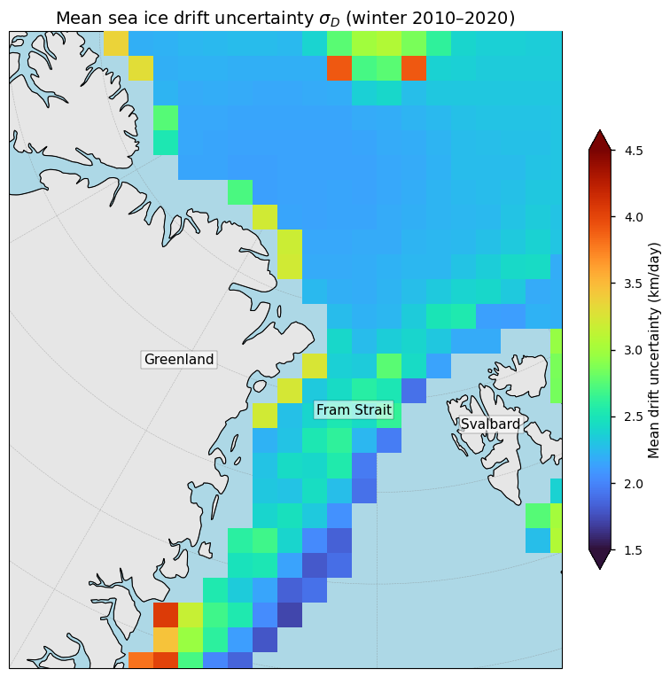
../../_images/11b7ca1826975b0f64b6ebdf1c690b32206a70cad300c623d4021fb6728c8aaf.png

Figure 3. Time-averaged sea ice drift uncertainty of the winter months (October-April) near the Fram Strait area between 2010-2020 of the C3S data.

The above figure shows the spatial pattern of the time-averaged uncertainty related to the sea ice drift data near the Fram Strait area. Uncertainties are lowest north of Fram Strait over closed sea ice, but clearly increase toward the dynamically active export region with peak values along the Greenland margin and near the sea ice edge. Let us plot some statistics (i.e. its minimum, maximum and average value) of the error variable over the entire domain:

uncert_dX_and_dY -> mean: 2.3066 km/day, min: 1.5718 km/day, max: 12.8355 km/day

This shows that a substantial variation is present in the uncertainty values data, but that the overall error meets the GCOS threshold of 5 km/day, as discussed before [5]. With this in mind, we can proceed to calculate the winter sea ice volume export through Fram Strait and its corresponding uncertainty.

3. Calculating the winter sea ice volume export through Fram Strait between 2010-2020#

3.1 Defining the location of the Fram Strait gate#

We define the gate as follows, which is a location similar to that of Ricker et al. (2018) [2]. The meridional gate is located along 82°N between 12°W and 20°E. The zonal part is located along 20°E between 80.5°N and 82°N. Let us define a function that extracts pixels that define the gate:

Show code cell source

Hide code cell source

def get_gate_pixels(ds):
    lat = ds["latitude"].values
    lon = ds["longitude"].values

    gate_mask_lat = (
        np.isclose(lat, 82.0, atol=0.4) &   # use wide tolerance for debugging
        (lon >= -14.0) &
        (lon <= 20.0)
    )
    gate_mask_lon = (
        (np.isclose(lon, 20.0, atol=2.0) | np.isclose(lon, 21.0, atol=2.0))
        &
        (lat >= 80.5) &
        (lat <= 82.0)
    )
        
    proj = ccrs.LambertAzimuthalEqualArea(central_longitude=0,
                                          central_latitude=90)

    fig, ax = plt.subplots(figsize=(8, 8), subplot_kw={"projection": proj})

    # Extent in lon/lat
    lon_min, lon_max = -30, 80      # degrees
    lat_min, lat_max = 75, 85       # degrees

    proj = ccrs.LambertAzimuthalEqualArea(central_longitude=0, central_latitude=90)

    xy_min = proj.transform_point(lon_min, lat_min, src_crs=ccrs.PlateCarree())
    xy_max = proj.transform_point(lon_max, lat_max, src_crs=ccrs.PlateCarree())

    xmin, ymin = xy_min
    xmax, ymax = xy_max
    ax.set_extent([xmin, xmax, ymin, ymax], crs=proj)

    # Land/ocean
    ax.add_feature(cfeature.OCEAN, facecolor="lightblue", zorder=0)
    ax.add_feature(cfeature.LAND, facecolor="0.9", edgecolor="black", zorder=1)
    ax.coastlines(linewidth=0.8, zorder=2)
    ax.gridlines(draw_labels=False, linewidth=0.4, linestyle="--",
                 color="gray", alpha=0.4)

    ax.scatter(
        lon[gate_mask_lat], lat[gate_mask_lat],
        transform=ccrs.PlateCarree(),
        color="red", s=60, zorder=10
    )
    ax.scatter(
        lon[gate_mask_lon], lat[gate_mask_lon],
        transform=ccrs.PlateCarree(),
        color="blue", s=60, zorder=10
    )

    #  Plot Fram Strait Gate: create geographic coordinate arrays
    lon_meridional = np.linspace(-12, 20, 200)    # 12°W to 20°E
    lat_meridional = np.full_like(lon_meridional, 82.0)  # constant 82°N
    lat_zonal = np.linspace(80.5, 82.0, 200)      # 80.5°N to 82°N
    lon_zonal = np.full_like(lat_zonal, 20.0)     # constant 20°E

    # Plot thick black lines
    ax.plot(
        lon_meridional, lat_meridional,
        color='black', linewidth=3,
        transform=ccrs.PlateCarree(), zorder=10
    )

    ax.plot(
        lon_zonal, lat_zonal,
        color='black', linewidth=3,
        transform=ccrs.PlateCarree(), zorder=10
    )

    # Construct legend
    meridional_proxy = plt.Line2D([], [], color='red', marker='o', linestyle='None',
                                  markersize=10, label='Meridional gate pixels')
    zonal_proxy = plt.Line2D([], [], color='blue', marker='o', linestyle='None',
                             markersize=10, label='Zonal gate pixels')

    # Add some text
    ax.text(-5, 81.25, "Fram Strait", transform=ccrs.PlateCarree(), fontsize=11, bbox=dict(facecolor="white", edgecolor="black", alpha=0.6, pad=2))
    ax.text(-35, 79, "Greenland", transform=ccrs.PlateCarree(), fontsize=11, bbox=dict(facecolor="white", edgecolor="black", alpha=0.6, pad=2))
    ax.text(12, 79, "Svalbard", transform=ccrs.PlateCarree(), fontsize=11, bbox=dict(facecolor="white", edgecolor="black", alpha=0.6, pad=2))
    
    ax.legend(handles=[meridional_proxy, zonal_proxy],
              loc="upper right",
              fontsize=11,
              frameon=True,
              facecolor="white",
              edgecolor="black")

    plt.title("Gate pixels Fram Strait", fontsize=14)
    plt.show()

    return gate_mask_lat, gate_mask_lon

Now we can plot those pixels:

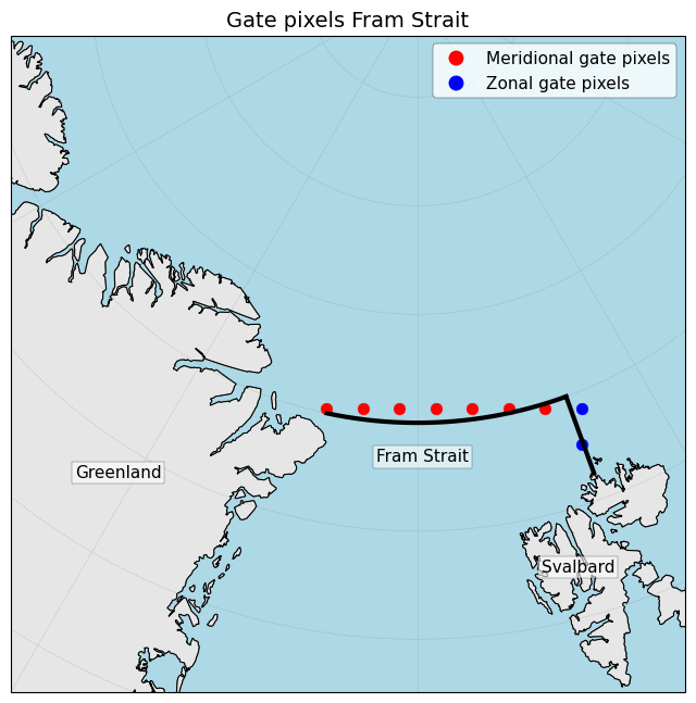
../../_images/2748fc33adcb0e27c28d873e83e9f98b1bdde4b6351daa1439ab0bdef7458441.png

Figure 4. The pixels that define the gate through which the sea ice volume flux is calculated. Note that the gate pixels and the actual gate are not aligned, implying that a correction has to be applied to the data to calculate the fluxes. The black lines follow the 82°N parallel and 20°E meridian, while the points denote the corresponding pixels that define the gate within the equal area projection grid.

These gate pixels are similar to the gate defined in Ricker et al. (2018) and Min et al. (2019) [2, 3]. We can now calculate the sea ice volume export through this gate by combining the C3S sea ice drift data with C3S ice thickness and ice concentration data.

3.2 Calculating winter sea ice export through the Fram Strait#

The sea ice volume flux transported through the defined gate is calculated by addressing the zonal and meridional part of the gate, similar to the procedure in Ricker et al. (2018) [2].

For the meridional part, this implies:

\( Q_V = L * H * C * D_V \)

where:

\(L\) = the length along the gate [km],

\(H*C\) = the effective sea ice thickness, as the product of the sea ice thickness \(H\) and sea ice concentration \(C\) [km],

\(D_V\) = the meridional component of the sea ice drift [km/day].

The procedure is similar for the zonal component \(Q_U\):

\( Q_U = L * H * C * D_U \)

It is important to note that the sea ice drift vector components provided in the satellite drift products are expressed relative to the native equal area grid projection rather than to true geographic directions. As a result, the reported X and Y components do not correspond directly to zonal (east-west) or meridional (north-south) motion in geographical space. To obtain physically meaningful drift components, a coordinate transformation must be applied that accounts for the grid projection geometry. Hence, the sea ice drift vectors must be rotated so that their components are expressed relative to the orientation of the gate (which is defined along a line of constant latitude and longitude) [7]:

\(D_V = D_x * sin(\lambda) - D_y * cos(\lambda)\), and

\(D_U = D_x * cos(\lambda) + D_y * sin(\lambda)\)

Also the gate length has to be corrected:

\(L = \dfrac{\Delta y}{cos(\lambda)}\) = \(\dfrac{\Delta x}{cos(\lambda)}\)

Here, \(\lambda\) is the longitude of the grid cell. The final total monthly export is then calculated as:

\(Q_{gate} = \sum\limits^{time} \sum\limits^{gate} Q_V + \sum\limits^{time} \sum\limits^{gate} Q_U\) [km\(^3\)/month]

Let us now perform this calculation:

Show code cell source

Hide code cell source

# Define variables
ds_drift = datasets["satellite-sea-ice-drift"]
ds_sit   = datasets["satellite-sea-ice-thickness"]
ds_conc  = datasets["satellite-sea-ice-concentration"]

# Align in time and space 
ds_drift, ds_sit, ds_conc = xr.align(ds_drift, ds_sit, ds_conc, join="inner")

# Monthly displacements along the x,y directions (km/month)
Dx = ds_drift["dX_sum"]      # (time, yc, xc)
Dy = ds_drift["dY_sum"]

# Sea ice concentration (fraction 0–1)
C  = ds_conc["ice_conc"] / 100.0

# Sea ice thickness (m)
H  = ds_sit["sea_ice_thickness"] / 1000.0   # m to km

# Effective thickness H*C in km
H_eff_km = (H * C) 

# Geographic longitude (degrees) and radians
lon_deg = ds_drift["longitude"]
lam = np.deg2rad(lon_deg)     # longitude in radians, same shape as grid

# Grid spacing in km (from xc,yc)
dx_nom = float(ds_drift["xc"].diff("xc").mean())   # km
dy_nom = float(ds_drift["yc"].diff("yc").mean())   # km

# Meridional (v) and zonal (u) components in geographic space, km/month
Dv = Dx * np.sin(lam) - Dy * np.cos(lam)
Du = Dx * np.cos(lam) + Dy * np.sin(lam)

# Avoid division by zero 
coslam = np.cos(lam)
coslam = xr.where(coslam == 0, np.nan, coslam)

# Grid cell lengths
Lv = dy_nom / coslam    # km, meridional gate segments
Lu = dx_nom / coslam    # km, zonal gate segments

# Volume fluxes
Qv_cell = Lv * H_eff_km * Dv    # (time, yc, xc) km³/month
Qu_cell = Lu * H_eff_km * Du

# Get gates
gate_mask_lat = xr.DataArray(
    gate_mask_lat, 
    dims=("yc", "xc"),
    coords={"yc": ds_drift.yc, "xc": ds_drift.xc}
)

gate_mask_lon = xr.DataArray(
    gate_mask_lon, 
    dims=("yc", "xc"),
    coords={"yc": ds_drift.yc, "xc": ds_drift.xc}
)

gate_mask_lat = gate_mask_lat.expand_dims(time=ds_drift.time).transpose("yc", "xc", "time")
gate_mask_lon = gate_mask_lon.expand_dims(time=ds_drift.time).transpose("yc", "xc", "time")

# Meridional part (only gate_mask_lat pixels)
Qv_gate = Qv_cell.where(gate_mask_lat).sum(dim=("yc", "xc"), skipna=True)

# Zonal part (only gate_mask_lon pixels)
Qu_gate = Qu_cell.where(gate_mask_lon).sum(dim=("yc", "xc"), skipna=True)

# Total export through Fram Strait gate
Q_total = Qv_gate + Qu_gate       # 1D over time, km³/month

With the calculation performed, we can now plot the data as a time series:

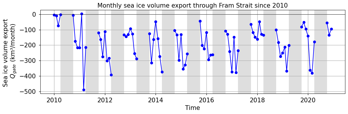
../../_images/885f42a7aa9e94551964178826768f3056853de735c8c1ad0fa253192b2056ad.png

Figure 5. Monthly sea ice volume export through Fram Strait obtained with C3S sea ice data. Here, we define negative values as outflow or export by convention. Shaded intervals indicate the summer months, during which data are not calculated.

The monthly sea ice volume export through Fram Strait derived from the C3S dataset exhibits substantial variability over the 2010–2020 period, with typical winter outflow rates ranging between approximately −100 and −400 km³ per month (with negative values indicating outflow or export by convention). Occasional extreme events occur, such as during March 2011, reflecting periods of strong ice drift and enhanced sea ice transport. The time series, in this notebook only spanning 10 years, shows some clear variability but no obvious long term trend, indicating that short-term atmospheric/oceanic forcing and seasonal ice conditions dominantly control the volume flux through Fram Strait during this time frame.

3.3 Sea ice volume export uncertainty#

To calculate the uncertainty with respect to the sea ice volume export, we follow the procedure in Ricker et al. (2018) [2]. This study expresses the pixel-by-pixel volume flux error estimate according to the law of error propagation. For a certain pixel, this implies:

\({\sigma_{Q}} = L \sqrt{(HC{\sigma_D})^2 + (HD\sigma_C)^2 + (DC\sigma_H)^2}\)

with \(L\) the gate length (km), \(H\) the sea ice thickness (km), \(C\) the sea ice concentration (-), and \(D\) the sea ice drift on a monthly basis (km/month). These symbols are also used as a subscript to express their corresponding uncertainty \(\sigma\).

We furthermore assume that the errors are uncorrelated in neither space nor time. This implies that, in order to calculate the monthly uncertainties of the sea drift data from the daily values, we take the square root of the sum of squares across all days within a month in a certain pixel:

\({\sigma_D} = \sqrt{\sum\limits^{N}_{d=1}{(\sigma_{D,d})^2}}\)

with \(N\) the number of days in a month and \(\sigma_{D,d}\) is the uncert_dX_and_dY variable for a certain day (km/day). Because a single uncertainty estimate is given per vector, we assume that \(\sigma_{D_V} = \sigma_{D_U}\).

We then calculate the total monthly volume flux uncertainty through all pixels of the gate as:

\({{\sigma_Q}_{gate}} = \sqrt{\sum\limits^{M}_{i=1}{(\sigma_{Q})^2}}\)

where \(M\) is the number of gate pixels.

Let us plot a time series of this data:

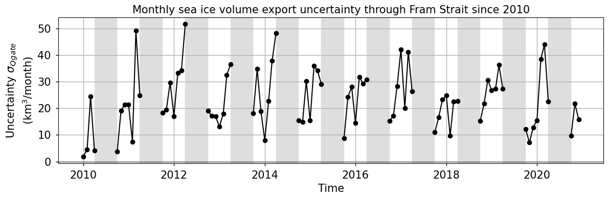
../../_images/ac99fb2ad24784bdb7e25c8372acf3b2df337752154c192b16e651f54178b22b.png

Figure 6. Monthly sea ice volume export uncertainties through Fram Strait obtained with C3S sea ice data. Shaded intervals indicate the summer months, during which data are not calculated.

Or when plotted as error bars on top of the actual data:

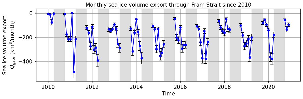
../../_images/93cd5dffbb316d73c168a855cdb909bb6a485bfcb7a459055814cf027e2697bf.png

Figure 7. Monthly sea ice volume export magnitudes through Fram Strait, together with their uncertainties shown as error bars, as obtained with the C3S sea ice data. Shaded intervals indicate the summer months, during which data are not calculated.

The error bars in the time series above illustrate the month-to-month uncertainty in the estimated sea ice volume export. Uncertainties typically range between roughly 10 and 50 km³ month⁻¹. The uncertainty varies over the record, which reflects changes in the quality of the underlying satellite observations. Overall, the magnitude of the error bars indicates that uncertainty represents a significant but not dominant fraction of the export signal, and that the C3S sea ice dataset quality is hence satisfactory. Moreover, since the uncertainty of the sea ice drift data are within acceptable GCOS bounds, as discussed earlier, the resulting volume export estimates can be considered robust. The error magnitude is not large enough to alter the overall variability or seasonal pattern of the export time series.

4. Comparison of Fram Strait volume fluxes with independent data#

4.1 Comparison of sea ice volume export with CMST data#

To evaluate the robustness of our calculated sea ice volume export, we compare our results with an independent dataset. Specifically, we use sea ice volume fluxes derived from the CMST product of Min et al. (2019) [3]. The CMST dataset generates spatio-temporal sea ice thickness fields in the Arctic and is produced with an Arctic regional ice–ocean model that assimilates remote sensing-derived values of sea ice thickness and concentration. In this system, grid cell-averaged sea ice thickness evolves according to the modelled thermodynamic growth and melt of sea ice and the sea ice flux divergence. Sea ice drift is needed to calculate these flux divergences, and is hence a byproduct of the model output. It is determined by the balance of internal ice stresses and wind and oceanic forcing [4]. Because the CMST framework provides modelled fields of ice drift, thickness, and concentration, its sea ice volume flux through Fram Strait offers an independent reference against which we compare our OSI SAF–based estimates.

Let us plot the comparison with data extracted from Min et al. (2019):

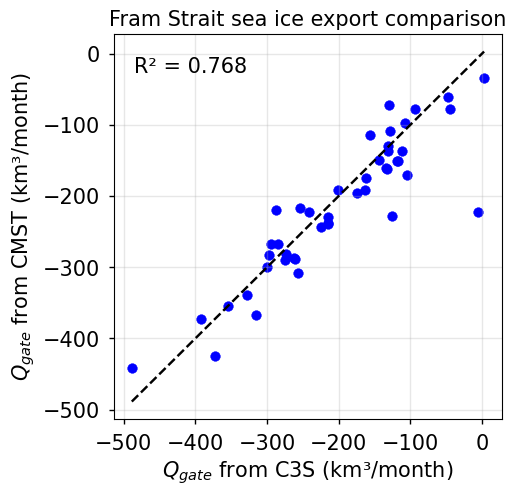
../../_images/7a3afc3544f869cb5c49efebf5af91ce15ca5698b6c813e5dba6cba9feaa2201.png

Figure 8. Comparison of C3S monthly sea ice volume export through Fram Strait with estimates from CMST data. The dashed line is the 1:1 line.

The comparison between monthly sea ice volume export through Fram Strait derived from C3S and CMST data shows a strong relationship, with an R\(^2\) = 0.768. Most data points cluster close to the 1:1 line, indicating that both products capture the variability and magnitude of the export fluxes quite well. The overall agreement demonstrates that the C3S retrievals provide a robust representation of monthly sea ice-related variables.

4.2 Comparison of sea ice volume export uncertainty with CMST data#

To check the credibility of the sea ice volume export uncertainties, we again compare the uncertainty estimates with those from an independent dataset. Specifically, we use sea ice volume flux uncertainties derived from the CMST product of Min et al. (2019) [3]. In CMST, uncertainties are quantified by the ensemble spread, that is, the standard deviation across ensemble members (i.e. 1 sigma precision errors, similar to our data). Let us plot the comparison with data extracted from Min et al. (2019):

Show code cell source

Hide code cell source

# Monthly uncertainty time series
sigma_monthly = sigma_Q_total.resample(time="1MS").mean()

# Mask only winter months (Oct–Apr)
winter_mask = sigma_monthly["time"].dt.month.isin([10, 11, 12, 1, 2, 3, 4])
sigma_winter = sigma_monthly.where(winter_mask)

# CMST data 
vals2 = np.array([
    np.nan, np.nan, np.nan, np.nan, np.nan, np.nan, np.nan, np.nan, np.nan,
    21, 23, 41, 14, 69, 15, 49,
    np.nan, np.nan, np.nan, np.nan, np.nan,
    24, 18, 42, 24, 39, 18, 21,
    np.nan, np.nan, np.nan, np.nan, np.nan,
    13, 16, 23, 12, 35, 22, 18,
    np.nan, np.nan, np.nan, np.nan, np.nan,
    16, 25, 34, 20, 15, 14, 13,
    np.nan, np.nan, np.nan, np.nan, np.nan,
    4, 17, 26, 31, 25, 31, 12,
    np.nan, np.nan, np.nan, np.nan, np.nan,
    18, 23, 24, 23, 12, 11, 8,
    np.nan, np.nan, np.nan, np.nan, np.nan,
    14, 13, 48
])

n = sigma_monthly.sizes["time"]
if len(vals2) < n:
    vals2 = np.pad(vals2, (0, n - len(vals2)), constant_values=np.nan)
else:
    vals2 = vals2[:n]

sigma_external = xr.DataArray(
    vals2,
    coords={"time": sigma_monthly["time"]},
    dims=["time"],
    name="sigma_external"
)

# Prepare plot
fig, ax = plt.subplots(figsize=(12, 4))

# Original series
sigma_winter.plot(ax=ax, color="black", marker="o", lw=1.5, label="C3S uncertainty")

# External series on top
sigma_external.plot(ax=ax, color="red", marker="s", lw=1.2, label="CMST uncertainty")

ax.set_ylabel(
    r"Uncertainty ${\sigma_Q}_{gate}$" "\n" r"(km$^3$/month)",
    fontsize=15
)
ax.set_xlabel("Time", fontsize=15)
ax.set_title("Monthly sea ice volume export uncertainty through Fram Strait since 2010", fontsize=15)

# Shade summer periods (May–September)
time_index = sigma_monthly["time"].to_index()
year_start = time_index.min().year
year_stop  = time_index.max().year

for year in range(year_start, year_stop + 1):
    ax.axvspan(
        pd.to_datetime(f"{year}-04-01"),
        pd.to_datetime(f"{year}-10-01"),
        color="lightgrey",
        alpha=0.75,
        zorder=0
    )

ax.axhline(0, color="k", lw=0.6)
ax.grid(True)
ax.tick_params(axis="both", labelsize=15)
ax.legend(fontsize=12)

plt.tight_layout()
plt.show()

../../_images/c963bf2eaa97f11783a84a440c76d61b163dd24e40cafcfec4f332187307766f.png

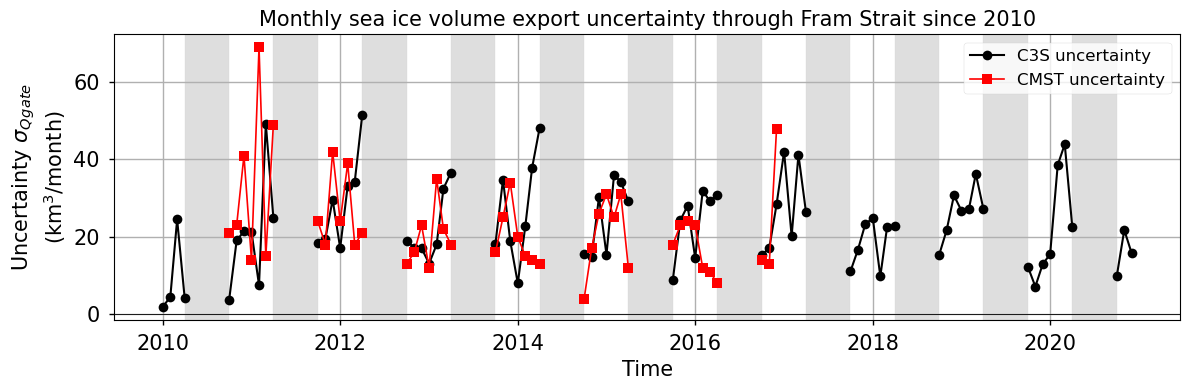
Figure 9. Monthly sea ice volume export uncertainties through Fram Strait obtained with C3S and CMST data. Shaded intervals indicate the summer months, during which data are not calculated.

The order of magnitude of the uncertainty estimate derived here is broadly consistent with the uncertainty reported by Min et al. (2019). For months where both estimates are available, the two methods yield uncertainties of the same order of magnitude (typically 15–35 km³ month⁻¹). Differences between the two estimates are generally within 5–15 km³ month⁻¹, corresponding to relative differences of approximately 20–40%. Let us quantify the exact values of the order of magnitude of the uncertainties over their overlapping period:

Mean C3S uncertainty: 24.37 km³/month
Mean CMST uncertainty: 22.98 km³/month

The uncertainty of the C3S data therefore appears consistent with independent uncertainty estimates for Fram Strait sea ice export and suggests that the overall uncertainty of the C3S monthly volume export is credible. This further supports the quality richness of the C3S data that are available on the CDS.

5. Short summary and take-home messages#

To be able to label a sea ice-related dataset as “quality rich” and for climate change analysis/monitoring to become reliable and possible, the dataset should at least exhibit a comprehensive spatial coverage (i.e. hemispheric), a long and continuous temporal coverage (> 30 years), quantified and transparent pixel-by-pixel uncertainty estimates that meet international proposed thresholds, a validation effort or a comparison to (theoretical) models, and an adequate spatio-temporal resolution (cfr. the “Maturity Matrix” [6]).

In that regard, the C3S sea ice drift dataset provides daily, pixel-by-pixel estimates of sea ice drift, together with associated quality flags and quantitative uncertainty estimates in the form of 1-sigma precision errors for both the Arctic and Antarctic region. In this notebook, the dataset was combined with C3S satellite-derived sea ice concentration and sea ice thickness products to compute the monthly winter sea ice volume export through Fram Strait. For that, all data were regridded and resampled to a common spatial and temporal frame, which limited the time period with valid data to the winter months of 2010-2020. Quality-wise, it can be stated that the spatial/temporal extent, the temporal resolution and the uncertainty characteristics of the sea ice drift product meet proposed GCOS requirements, implying a quality-rich dataset with respect to those aspects [5]. However, the spatial resolution of 75 km remains slightly too coarse with respect to internationally proposed thresholds: for GCOS, for example, the minimum threshold is 50 km. Despite this minor limitation, the resulting sea ice volume export estimates and their uncertainties show a good agreement with independent CMST-derived fluxes, indicating that the C3S sea ice drift product is sufficiently robust and credible for large-scale sea ice transport studies.

We further note, however, that this notebook deals with only a specific subset of the sea ice drift data, i.e. for the Fram Strait region and for the winter months of 2010-2020. This was done due to constraints of other C3S sea ice products, as well as to align the data with the temporal window of independent data reported in the literature [3]. The full dataset spans a broader spatial and temporal extent.

ℹ️ If you want to know more#

Key resources#

“Sea ice drift daily gridded data derived from satellite observations” on the CDS
Documentation on the CDS (Copernicus Knowledge Base).
Copernicus climate change indicators: sea ice
C3S EQC custom functions, c3s_eqc_automatic_quality_control prepared by B-Open.

References#

[1] Lavergne, T. and Down, E. (2023). A climate data record of year-round global sea-ice drift from the EUMETSAT Ocean and Sea Ice Satellite Application Facility (OSI SAF), Earth Syst. Sci. Data, 15, 5807–5834, https://doi.org/10.5194/essd-15-5807-2023
[2] Ricker, R., Girard-Ardhuin, F., Krumpen, T., and Lique, C. (2018). Satellite-derived sea ice export and its impact on Arctic ice mass balance, The Cryosphere, 12, 3017–3032, https://doi.org/10.5194/tc-12-3017-2018
[3] Min, C., Mu, L., Yang, Q., Ricker, R., Shi, Q., Han, B., Wu, R., and Liu, J. (2019). Sea ice export through the Fram Strait derived from a combined model and satellite data set, The Cryosphere, 13, 3209–3224, https://doi.org/10.5194/tc-13-3209-2019
[4] Mu, L., Losch, M., Yang, Q., Ricker, R., Losa, S. N., and Nerger, L. (2018). Arctic-Wide Sea Ice Thickness Estimates From Combining Satellite Remote Sensing Data and a Dynamic Ice-Ocean Model with Data Assimilation During the CryoSat-2 Period, J. Geophys. Res-Oceans, 123, 7763–7780, https://doi.org/10.1029/2018JC014316
[5] GCOS (Global Climate Observing System) (2022). The 2022 GCOS ECVs Requirements (GCOS-245). World Meteorological Organization: Geneva, Switzerland. doi: https://library.wmo.int/idurl/4/58111
[6] Yang, C. X., Cagnazzo, C., Artale, V., Nardelli, B. B., Buontempo, C., Busatto, J., Caporaso, L., Cesarini, C., Cionni, I., Coll, J., Crezee, B., Cristofanelli, P., de Toma, V., Essa, Y. H., Eyring, V., Fierli, F., Grant, L., Hassler, B., Hirschi, M., Huybrechts, P., Le Merle, E., Leonelli, F. E., Lin, X., Madonna, F., Mason, E., Massonnet, F., Marcos, M., Marullo, S., Muller, B., Obregon, A., Organelli, E., Palacz, A., Pascual, A., Pisano, A., Putero, D., Rana, A., Sanchez-Roman, A., Seneviratne, S. I., Serva, F., Storto, A., Thiery, W., Throne, P., Van Tricht, L., Verhaegen, Y., Volpe, G., and Santoleri, R. (2022). Independent Quality Assessment of Essential Climate Variables: Lessons Learned from the Copernicus Climate Change Service, B. Am. Meteorol. Soc., 103, E2032–E2049, https://doi.org/10.1175/Bams-D-21-0109.1
[7] Lavergne, T. (2023). Transformation and Rotation of OSI SAF Sea Ice Drift vectors (v1.0.0). Zenodo. https://doi.org/10.5281/zenodo.8398399

Sea ice drift from satellite observations: resolution and uncertainty of Arctic sea ice drift for large-scale sea ice transport analysis

Contents

1.3.11. Sea ice drift from satellite observations: resolution and uncertainty of Arctic sea ice drift for large-scale sea ice transport analysis#

🌍 Use case: Quantifying sea ice transport out of the Arctic Ocean through Fram Strait#

❓ Quality assessment question#

📢 Quality assessment statements#

📋 Methodology#

Dataset description#

Structure and (sub)sections#

📈 Analysis and results#

1. Data preparation and processing#

1.1 Import packages#

1.2 Define request and download#

1.3 Display and inspect data#

2. Patterns of sea ice motion and its uncertainty#

2.1 Average sea ice drift velocities#

2.2 Sea ice drift uncertainty#

3. Calculating the winter sea ice volume export through Fram Strait between 2010-2020#

3.1 Defining the location of the Fram Strait gate#

3.2 Calculating winter sea ice export through the Fram Strait#

3.3 Sea ice volume export uncertainty#

4. Comparison of Fram Strait volume fluxes with independent data#

4.1 Comparison of sea ice volume export with CMST data#

4.2 Comparison of sea ice volume export uncertainty with CMST data#

5. Short summary and take-home messages#

ℹ️ If you want to know more#

Key resources#

References#