

1.1.1. Cloud type determination for climate studies#
Production date, after final revision: 2026-06-02.
🌍 Use case: Monitoring cloud amount and relative occurrence of specific cloud types#
❓ Quality assessment question#
How well are the decadal changes in high-level cloud types represented in the CLARA-A3 satellite dataset ?
Clouds are fundamental regulators of the Earth’s climate system, significantly influencing the hydrological cycle, the atmospheric circulation and the Earth’s heat balance. These factors, in turn, play a crucial role in shaping ecosystems, agriculture, water resources, and weather patterns. The overall impact of clouds on Earth’s climate is determined by their physical properties, including their amount, their height, and their opacity (how much the cloud blocks sunlight and traps heat). The following notebook essentially focuses on the occurrence of high-level clouds, easiest observed from space, and which have important atmospheric radiative effects: they strongly trap outgoing longwave radiation from the Earth’s surface. While high opaque clouds strongly reflect solar radiation, thin cirrus allow most solar radiation to pass. The net radiative effect of high-level clouds therefore depends on their opacity, given by the optical thickness. Furthermore, a change in the geographical patterns of their relative occurrence leads to changes in the atmospheric circulation and thus in precipitation patterns.
This analysis uses cloud observations from the dataset Cloud properties global gridded monthly and daily data from 1979 to present derived from satellite observations, available in the Climate Data Store (CDS). Two complementary Thematic Climate Data Records of cloud properties are provided by two product families: CLARA-A3 (CMSAF cLoud, Albedo and surface Radiation) based on measurements by the Advanced Very High Resolution Radiometers (AVHRR), and CCI (Climate Change Initiative), based on measurements by the (Advanced) Along-Track Scanning Radiometers ((A)ATSR). The latter record has been extended in time using measurements by the Sea and Land Surface Temperature Radiometers (SLSTR). The data of these two product families differ in temporal sampling, horizontal resolution and methods to retrieve cloud properties.
In order to define cloud types according to height and opacity, this notebook uses Joint Cloud Histograms (JCH). These provide monthly cloud occurrence statistics within 13 x 15 two-dimensional intervals in Cloud Optical Thickness (COT) and Cloud-Top Pressure (CTP), averaged over grid cells of 1° latitude x 1° longitude. At the moment of creating this notebook, the CDS provides JCHs only for CLARA-A3. When JCHs are also available for CCI, these can be used similarly.
This notebook gives examples how these JCHs can be used to study the relative occurrence of specific cloud types. We first compare the geographical cloud type distributions of CLARA-A3 with those obtained from other cloud retrievals. Then, the interannual variability of the tropical relative occurrence of three different high-level cloud types (high opaque, cirrus and thin cirrus) is shown, and finally we explore their geographical anomaly patterns with respect to global surface temperature changes.
In this notebook, we define high-level clouds as clouds with a cloud-top pressure < 310 hPa. This corresponds to a height of about 10 km in the tropics and 8.5 - 9 km in the midlatitudes. They are then further distinguished as thin cirrus, cirrus and high opaque clouds, using COT thresholds of 1.3 and 9.4, respectively. This cloud type identification corresponds to the one applied in the updated Global Energy and Water Exchanges (GEWEX) cloud assessment [3], which has recently inter-compared 11 publicly available global cloud data records derived from measurements of multi-spectral imagers, IR sounders, and lidar.
The CLARA-A3 cloud detection relies on a Bayesian approach, by linking measurements from all AVHRR channels to the cloud detection from the Cloud-Aerosol Lidar and Infrared Pathfinder Satellite Observation mission (CALIPSO)[1] as a reliable reference. CTP is retrieved based on a neural network approach, trained on CALIPSO cloud-top height observations. In a second step, it is transformed to cloud-top height and temperature by applying atmospheric profiles from meteorological reanalyses. Ice clouds are distinguished from liquid clouds by considering spectral infrared brightness temperature differences. COT is only retrieved during daytime, using look-up tables (LUTs) based on visible and near-infrared reflectances and radiative transfer [2]. Therefore, the JCHs are also only available during daytime.
📢 Quality assessment statement#
It is important to note that passive remote sensing has limitations: it provides a top-down perspective, which does not account for hidden cloud layers, and classical retrievals, based on radiative transfer, estimate a ‘radiative’ cloud height. This radiative height can be several kilometers below the actual cloud top, especially in cases where clouds have diffuse tops, with optical depth gradually increasing from the top down over a significant vertical range. This phenomenon is relevant for approximately 70% of high clouds in the tropics and 30-40% of high clouds in the midlatitudes [4].
To overcome this problem, recent retrievals, such as the one developed for CLARA-A3, directly obtain the cloud-top height by using neural networks which have been trained on the cloud-top height derived by active lidar (CALIOP).
One has also to keep in mind that the retrieved optical thickness depends on the footprint of the initial measurement, since for the cloud property retrieval the whole footprint is assumed to be completely cloud-covered. Therefore, smaller instrument footprints should in general lead to larger Cloud Optical Thickness. This has an influence on the relative distribution between high opaque, cirrus and thin cirrus clouds.
These are the key outcomes of this assessment
Over the tropics, according to CLARA-A3, high-level clouds make up about 55% of all clouds over ocean and 65% over land. These values are in agreement with active lidar retrievals by the CALIPSO Science Team. However, one has to keep in mind that active lidar is more sensitive to thin cirrus clouds than passive instruments.
When CLARA-A3 classifies these tropical high-level clouds by opacity, over ocean (land) about 20 (30) % of them are opaque, while 45 (55) % of them are cirrus clouds while 35 (15) % of them are thin cirrus clouds. These results are similar to the ones retrieved from the MODIS continuity retrieval. In contrast, other satellite datasets do not show a difference in thin cirrus coverage between land and ocean. This reflects the difficulty of detecting thin cirrus over land.
The tropical annual mean time series over the whole period (1980-2020) are only stable for maritime high opaque clouds. For other high-level cloud types, stable records only exist for 2003-2015, when observation times are coherent, with two daytime measurements at around 10 AM and 1:30 PM local time. Outside this period, changes in observation times reduce temporal stability. Even over the coherent observation time period 2003-2015, CLARA-A3 shows a slight relative increase of all high-level cloud types, which is not confirmed by other cloud data records. The present data provide statistics merged over all available daytime observation times. For monitoring purposes, using single consistent overpasses (e.g., 1:30 PM +/-1 h) are easier to interprete.
During the period of consistent observation times (2003-2015), spatial patterns of cloud type changes in response to surface temperature anomalies show increases near the equator in the tropical Pacific and decreases over Indonesia, consistent with El Nino-Southern Oscillation (ENSO) effects. Thin cirrus amounts also increase near the equator alongside high opaque clouds, reflecting the growth of tropical mesoscale convective systems and their surrounding cirrus. These results are in agreement with the ones using other datasets.
📋 Methodology#
The analysis comprises the following steps:
Choose the parameters to use and setup code
Import the relevant libraries.
Define the parameters of the analysis and set the dataset requests.
Prepare the datasets for the analysis, first aggregating statistics of liquid and ice clouds, then grouping the initial CTP and COT intervals of the JCHs into three each. This leads to nine cloud types based on the cloud optical thickness (COT) and cloud Top Pressure (CTP).
Download the CLARA-A3 monthly mean JCHs and the reanalysis ERA5 land sea mask available on CDS.
Download the Southern Oscillation Index (SOI) obtained from National Centers for Environmental Information.
Plot geographical maps (60°N-60°S) of the normalized occurrence frequency of these nine cloud types, averaged over the period 2008-2015.
Split sea and ocean data using a land sea mask.
Plot time series of tropical cloud amount, relative proportion of high-level clouds (CTP < 310 hPa) and of thin cirrus, cirrus and high opaque clouds, separately over ocean and land.
Plot time series of SOI and global mean surface temperature anomalies.
Compute, per 1° grid cell, linear regression slopes of deseasonalized monthly mean anomalies in relative amount of thin cirrus, cirrus and high opaque clouds with respect to deseasonalized global mean surface temperature anomalies, for the period 2003-2015 over 40°N-40°S. The surface temperature anomalies are given by GISTEMP Team 2023 [5].
Plot their geographical distributions.
📈 Analysis and results#
Choose the parameters to use and setup code#
This section includes the library imports and the parameter settings for the analysis.
Import libraries#
Set parameters#
Define request#
two datasets are requested from the CDS:
Joint Cloud Histogram (JCH)
Land Sea Mask (LSM)
One dataset is requested from the NASA website:
Southern Oscillation Index (SOI)
Define functions to cache#
Download and transform#
collection_id='satellite-cloud-properties'
100%|██████████| 41/41 [00:21<00:00, 1.91it/s]
collection_id='reanalysis-era5-single-levels'
100%|██████████| 1/1 [00:00<00:00, 12.83it/s]
Results#
For a better comparison with results of the updated GEWEX cloud assessment [3], we have grouped the JCH statistics of the original 13 x 15 COT-CTP intervals into 3 x 3 COT-CTP intervals. These intervals correspond to nine cloud types classified according to opacity (COT thresholds 1.3 and 9.4) and height (CTP thresholds 310 hPa and 680 hPa).
Relative Occurrence of Specific Cloud Types#
Figure 1 presents the normalized occurrence frequencies of the nine cloud types obtained by dividing the statistics of the grouped JCHs by the statistics summed over all JCH intervals, for each 1° grid cell. These maps allow to quickly visualise specific geographical patterns such as tropical thin cirrus (top left, cloud type interval (1.1)), tropical cirrus anvils (top center, cloud type interval (2.1)) or Stratocumulus (bottom center, cloud type interval (2.3)) regions off the Western coasts.
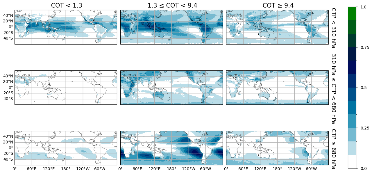
Figure 1: Geographical distributions (60°N-60°S) of normalized occurrence frequency of nine cloud types from CLARA-A3, distinguished by Cloud Optical Thickness (COT), with thresholds at 1.3 and 9.4, and Cloud Top Pressure (CTP), with thresholds at 310 and 680 hPa. Statistics averaged over day-time from 2008 to 2015.
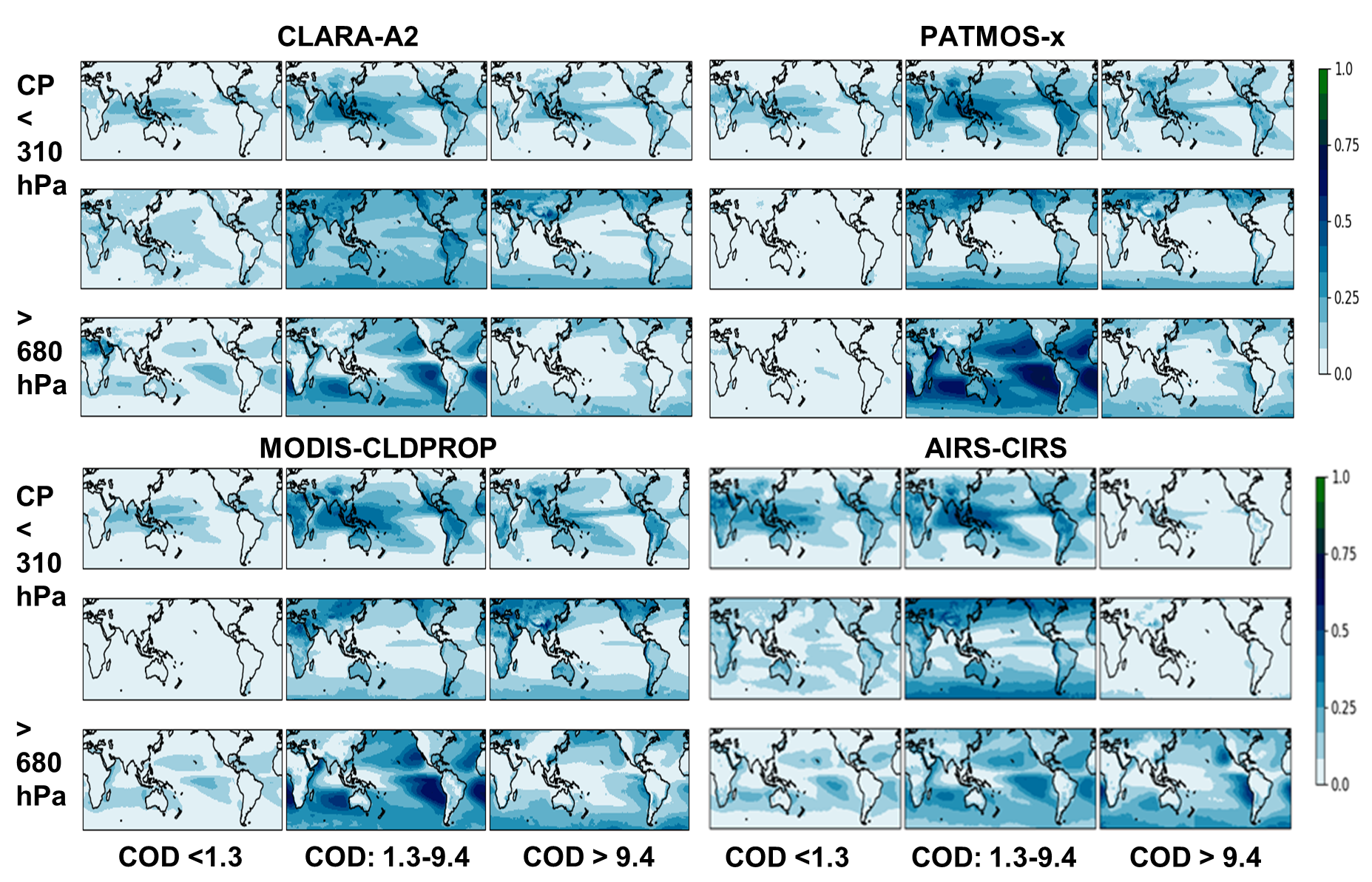
Figure 2 : Geographical distributions (60°N-60°S) of normalized occurrence frequency of nine cloud types distinguished by COD (horizontal axis) and CP (vertical axis) from CLARA-A2, PATMOS-x, MODIS-CLDPROP and AIRS-CIRS. Statistics averaged over 1:30PM LT from 2008 to 2015. Subset of panels extracted from Figure 10 of Stubenrauch et al. 2024 [3]
The comparison of Figure 1 with the maps of four datasets presented in Figure 10 of [3], and extracted as Figure 2 in this notebook, leads to the following assessment of CLARA-A3: Compared to CLARA-A2 (V2.0), CLARA-A3 provides more high-level and less mid-level clouds. This can be easily explained by the fact that the CLARA-A3 neural network retrieval, trained on lidar data, estimates the cloud top, while the classical CLARA-A2 retrieval estimates the lower ‘radiative’ cloud height. Another difference can be noticed for the Stratocumulus clouds off the Western coasts, which seem to have a more structured occurrence, again due to the new neural network approach linked to lidar height.
The geographical patterns of the normalized occurrence of tropical thin cirrus given by CLARA-A3 are similar to the ones given by AIRS-CIRS [6], though with less thin cirrus over land. This shows an improvement compared to CLARA-A2, as IR sounders such as AIRS identify thin cirrus reliably.
The geographical patterns of cirrus are similar to those of PATMOS-x [7] using the same AVHRR measurements, MODIS-CLDPROP [8] using the MODIS Science Team cloud property continuity retrieval, and AIRS-CIRS, with maxima of cirrus anvils above the most convective regions, above Indonesia, South America and Africa. However, CLARA-A3 presents more of these higher thicker clouds in the midlatitudes. This can be explained again by the fact that the neural network retrieval places the high-level clouds close to the tropopause, while the retrievals based on radiative transfer place the clouds lower (see also the notebook ‘Intercomparison of cloud-top pressure distributions derived from satellite observations’).
Interannual variability#
The JCHs also include the cloud area fraction for each 1° grid cell. Since the JCHs include only cloudy statistics, this variable can be used as a weight in order to transform relative occurrences into absolute occurrences. In the following, we consider time series of total cloud amount and relative cloud type amounts, separately over ocean and over land.
The upper panels of Figure 3 present time series of the tropical annual mean cloud amount (CA), computed as the average over the latitude band 25N-25S of the annual mean fractional cloud cover per 1° grid. These curves can be directly compared to the results of the updated GEWEX cloud assessment reproduced in Figure 4.
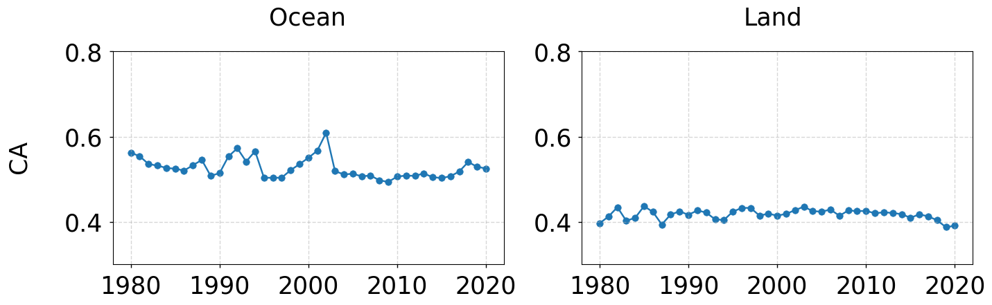
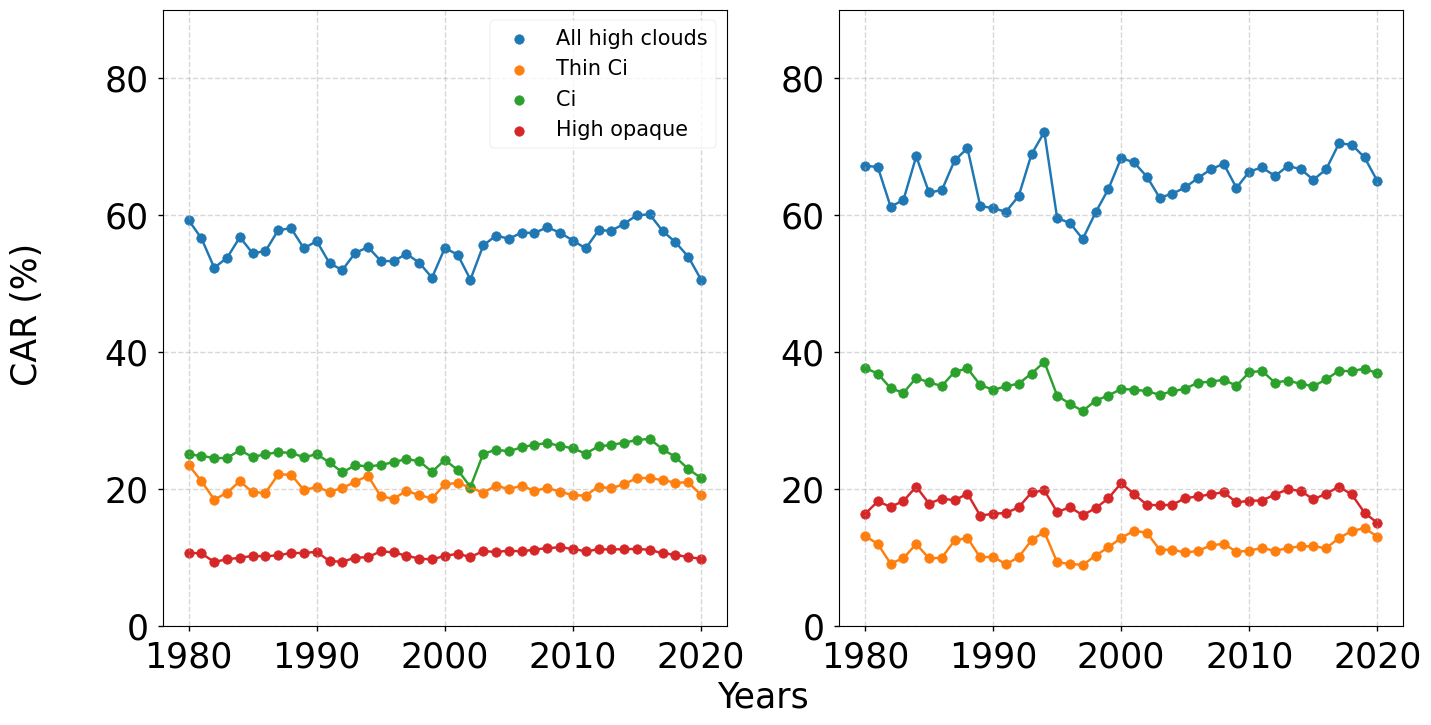
Figure 3: Time series of annual means of (top) tropical cloud amount and (bottom) relative proportion of all high-level clouds (CTP < 310 hPa, blue), thin cirrus (Thin Ci, orange), cirrus (Ci, green) and high opaque clouds (red), separately over ocean (left) and over land (right). Statistics averaged over 25N – 25S, for 1980 - 2020, during daytime. Only during the period 2003-2015, two observation times are used homogeneously at around 10AM and 1:30PM local time. Before that period, only afternoon observations are used, which have been less stable in time, and afterwards only morning observations, as the afternoon observations strongly drifted in time.
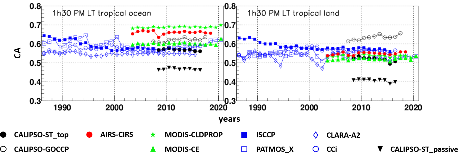
Figure 4: Time series of cloud amount, over tropical ocean (left) and tropical land (right). Statistics at 1:30PM LT over 25N-25S. The colours correspond to specific instrument types (black: active lidar, red: IR sounders, green: advanced multi-spectral imagers, blue: multi-spectral imagers). Subset of panels extracted from Figure 12 of Stubenrauch et al. 2024 [3]
The time series of tropical CA shown on the upper panel of Figure 3, is more stable over land than over ocean, the latter showing two significant increases in the early 1990’s and in 2002. These increases over ocean also appear in the tropical CA of PATMOS-x (Figure 4), while other data records, including CLARA-A2, do not show this behaviour. This can be explained by the fact that PATMOS-x and CLARA-A3 use a similar cloud detection method. The tropical CA of CLARA-A3 over ocean (Figure 3 upper panels) is about 0.1 higher than over land, in agreement with AIRS-CIRS, CALIPSO-ST (retrieval by CALIPSO Science Team) and MODIS-CE (retrieval by MODIS CERES Science Team, [15]. However, while CLARA-A3 and CLARA-A2 (V2.1) provide a similar cloud cover in the tropical latitude bands in the notebook ‘Satellite cloud cover validation for Climate modelling’, the cloud amount of CLARA-A3 over tropical land seems to be slightly underestimated, with about 0.4, compared to about 0.5 from CLARA-A2 (V2.0) and all other retrievals using AVHRR measurements. It is interesting to note that the CA over tropical land of CALIPSO-ST_passive, which simulates a CA of clouds with COT > 0.3, is also only 0.4. This indicates that CLARA-A3 has problems to detect / identify thin clouds over land.
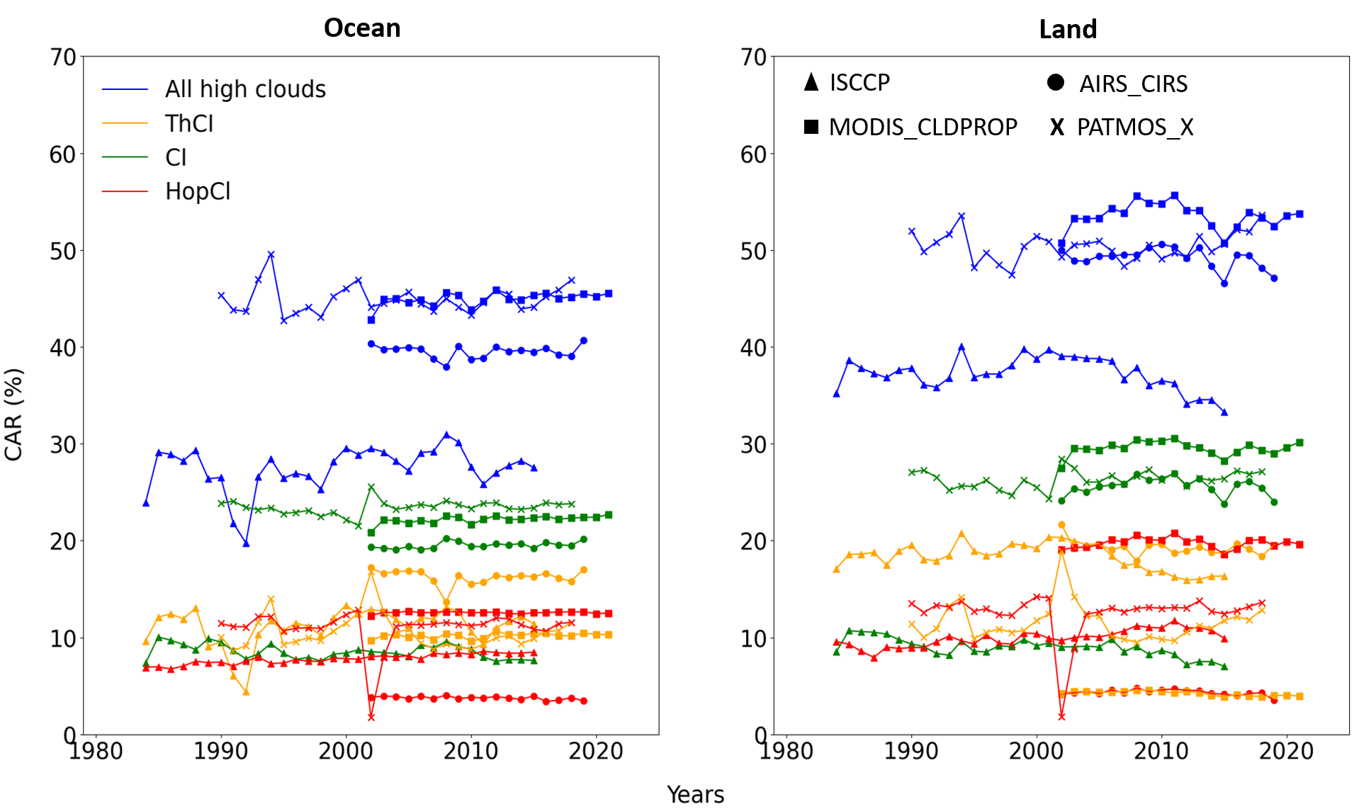
Figure 5: Time series of relative proportion of all high-level clouds (CTP < 310 hPa, blue), thin cirrus (Thin Ci, orange), cirrus (Ci, green) and high opaque clouds (red), separately over ocean (left) and over land (right). Statistics averaged over 25N – 25S, for 1980 - 2020, during daytime. The markers correspond to the following datasets AIRS-CIRS, ISCCP, MODIS-CLDPROP and PATMOS-x. Data from updated GEWEX cloud assessment database (available at https://gewexca.aeris-data.fr/datasets/ ).
The lower panels of Figure 3 present time series of the tropical annual mean amount of all high-level clouds (blue), as well as of thin cirrus (orange), cirrus (green) and high opaque clouds (red), relative to all clouds, again separately over ocean and over land. The threshold of 310 hPa corresponds in the tropics to a height of about 10 km. The relative amount of high-level clouds from CLARA-A3 is relatively large and compares well with the one of CALIPSO-ST, with about 60% and 70% respectively. However, the interannual variability has not the same behaviour. It was already pointed out in [3] that it is very difficult to observe cloud trends within latitudinal bands using currently available cloud data records. Furthermore, the AVHRR cloud products, existing over a 40-year period, are more stable after 2003. The CLARA-A3 time series also show differences in behaviour between the periods before and after 2003 (Figure 3 lower panels). This can be explained by the observation times which have been used to create the CLARA-A3 JCHs: Only during the period 2003-2015, two observation times are used homogeneously at around 10AM and 1:30PM local time. Before that period, only afternoon observations are used, which have been less stable in time, and afterwards only morning observations, as the afternoon observations strongly drifted in time.
For a comparison of the time series of the three high-level cloud type occurrences, we have analysed the JCHs of the updated GEWEX cloud assessment database, by applying the same CTP and COT thresholds as for this analysis and the results are shown in Figure 5.
The most stable CLARA-A3 relative amount is the one of maritime tropical high opaque clouds, of about 11% (Figure 3 lower left panel). The continental tropical relative high opaque cloud amount is nearly twice as large (about 18%) and less stable (Figure 3 lower right panel). The largest relative amount is the one of tropical cirrus, with 25% over ocean and 35% over land. The relative amount of tropical thin cirrus shows an opposite behaviour, with 20% over ocean and only 10% over land. These results are similar to the ones of MODIS-CLDPROP, though with larger absolute values, as the high-level cloud amount is about 15% larger for CLARA-A3. However, PATMOS-x, also based on AVHRR measurements, does not show any difference between tropical ocean and land for thin cirrus and high opaque clouds (Figure 5).
According to CLARA-A3, the relative amount of all three high-level cloud types slightly increases since the 2000’s (Figure 3 lower panels). However, this behaviour is not observed in the other datasets (PATMOS-x, MODIS-CLDPROP and AIRS-CIRS, Figure 5).
Anomaly Patterns linked to the Global Surface Temperature#
As it is difficult to observe cloud trends, in particular over a time period which is short for climate change attribution, we explore in this part of the notebook how regional patterns change with respect to interannual global surface temperature variability.
The global surface temperature reflects global warming, but large interannual changes are related to episodes of El Niño (warm) and La Niña (cool), as is illustrated in Figure 6, which presents the time series of deseasonalised global mean surface temperature anomalies (black curve, left axis) and the Southern Oscillation Index (SOI, right axis, with red and blue indicating El Niño and La Niña episodes, respectively). These data are obtained from the GISS Surface Temperature Analysis (for global mean surface temperature anomalies) and the NOAA website (for the SOI).
It is interesting to note that during the period before 2003 the global surface temperature anomalies are all negative, in particular between 1982 and 1992. Indeed, there has been a climate warming during the last four decades, but these negative anomalies may be partly explained by aerosol dimming [16] and the Mount Pinatubo eruption in 1991.
For the following analysis of regional cloud type variability patterns with respect to inter-annual global mean surface temperature anomalies, we concentrate on the period 2003-2015, for which the observation times of the CLARA-A3 JCHs are coherent.
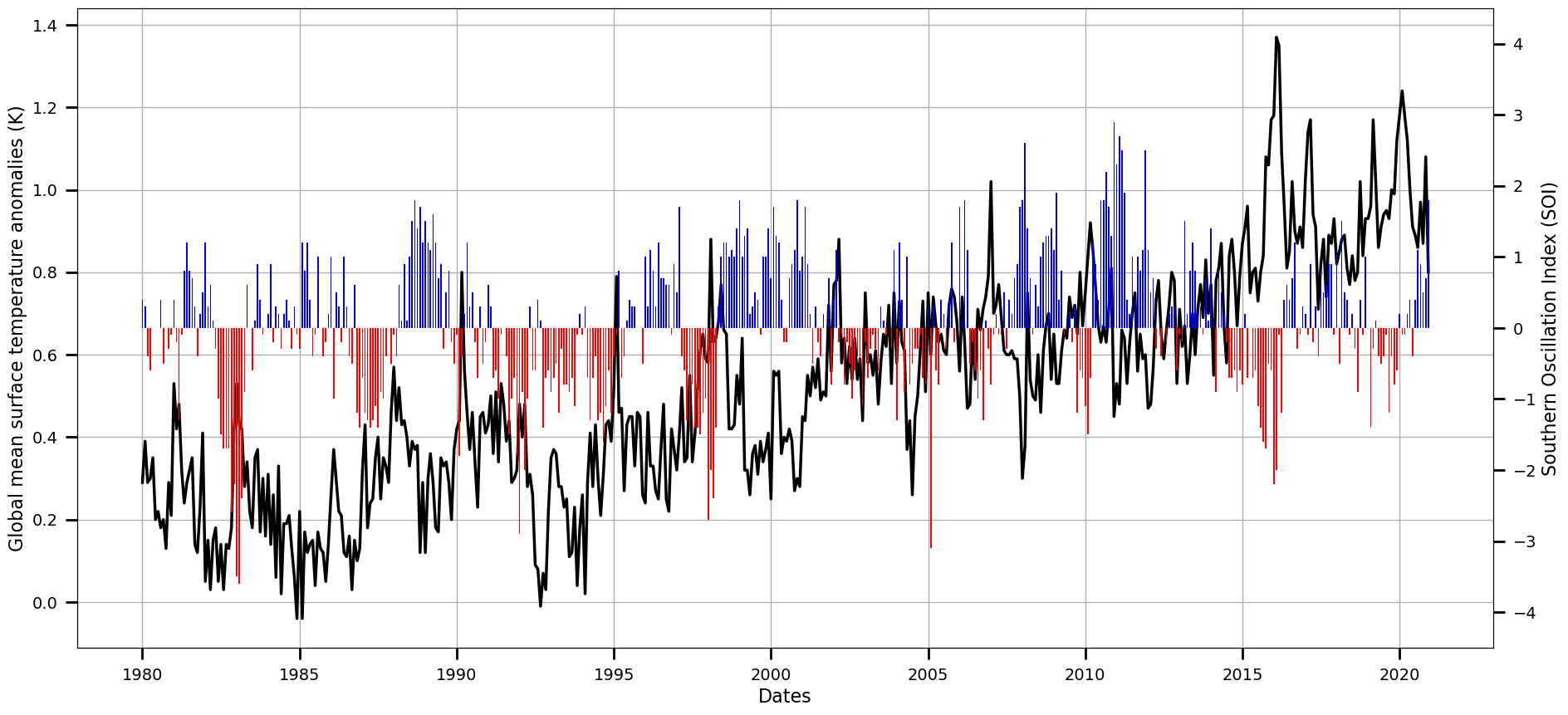
Figure 6: Time series of deseasonalised global mean surface temperature anomalies (black, left axis) and Southern Oscillation Index (SOI) (right axis), made with available data on NOAA website. The colors red and blue correspond to El Niño and La Niña episodes, respectively.
The monthly deseasonalized 1° x 1° relative cloud type amount anomalies and global surface temperature anomalies are obtained by subtracting the monthly mean (at 1° resolution and global, respectively) over the whole period, 2003 – 2015.
Then, we determine geographical change patterns in amount of these cloud types, relative to all clouds, with respect to global surface temperature change by calculating the linear regression slopes of the ratio between relative cloud type amount anomaly and global surface temperature anomaly, per grid cell.
We use the same method as was used in the updated GEWEX cloud assessment, so that the results presented in Figure 7 can be directly compared to Figure 13 of [3], copied to Figure 8 of this notebook. Indeed, one could have used a more sophisticated statistical method, but these figures serve just as an illustration.
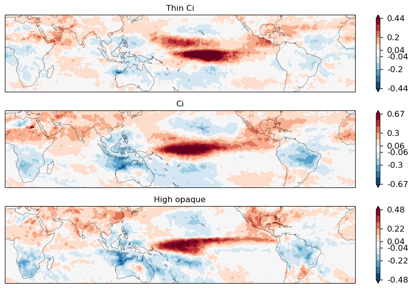
Figure 7: Geographical maps of linear regression slopes between monthly mean anomalies in amount of thin cirrus (left), cirrus (middle) and high opaque clouds (right), relative to all clouds, and global mean surface temperature anomalies, during the period 2003-2015, over 40°N-40°S. Units are in fractional change per °C warming. The global mean surface temperatures are given by the GISS Surface Temperature Analysis [9].
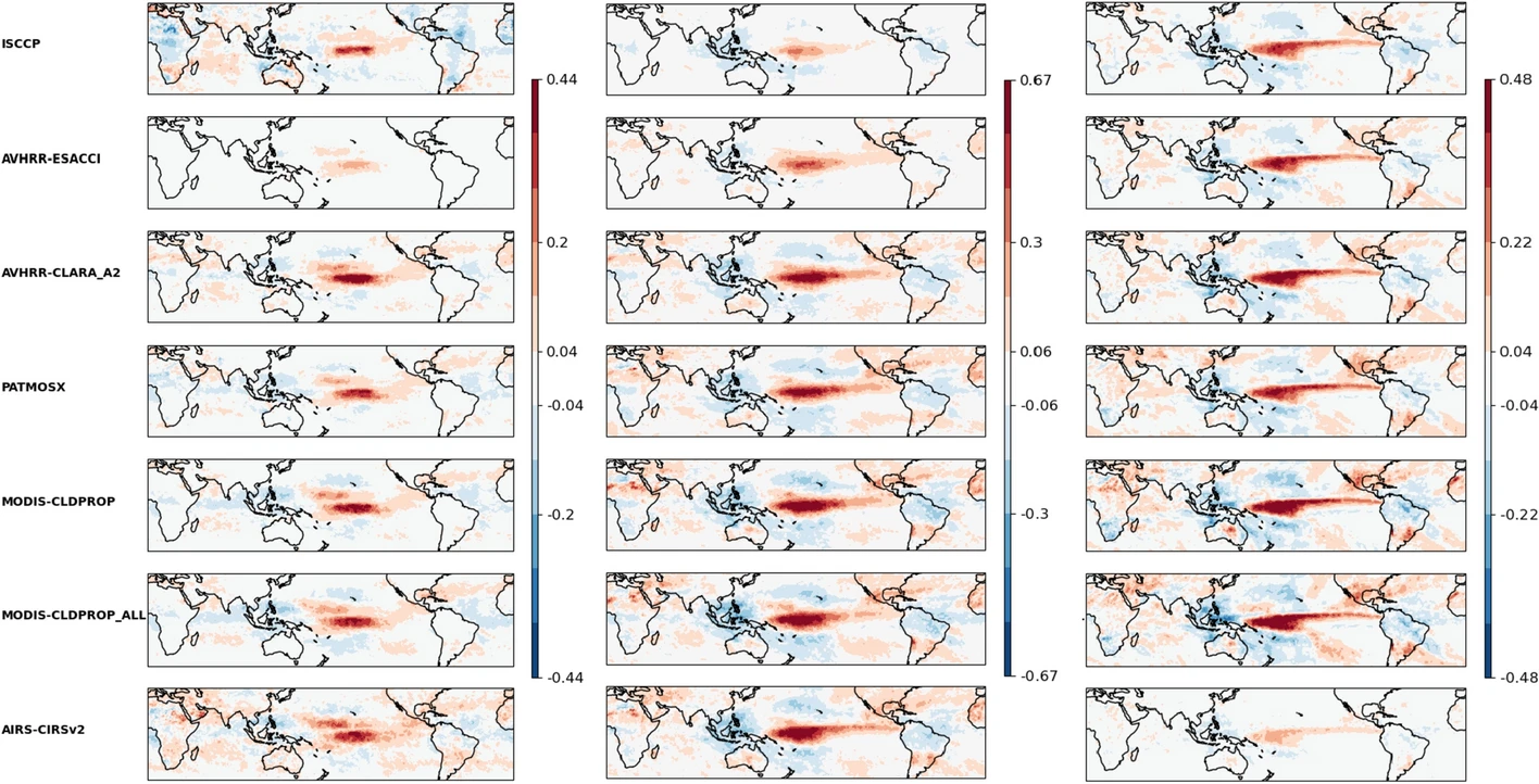
Figure 8: Geographical maps of linear regression slopes between monthly mean anomalies in amount of thin cirrus (left), cirrus (middle) and high opaque clouds (right), relative to all clouds, and global mean surface temperature anomalies. Units are in fractional change per °C warming. Cloud data are from ISCCP, AVHRR-Cloud_cci, AVHRR-CLARA (CLARA-A2), PATMOS-x, MODIS-CLDPROP_ALL, MODIS-CLDPROP and AIRS-CIRS (from top to bottom), and surface temperature from the GISS Surface Temperature Analysis, during the period 2003–2015, 40N-40S. Source: Stubenrauch et al. 2024 [3].
CLARA-A3 shows a relative increase per °C of warming of all these three cloud types near the equator in the tropical Pacific and a decrease over Indonesia, similar to the cloud datasets in the updated GEWEX cloud assessment and similar the pattern caused by the El Niño–Southern Oscillation (ENSO [10]).
We also observe an increase in cirrus and thin cirrus in the subtropics. This may be in relation to a hypothesized widening of the Hadley cell with global warming [11].
The relative amount of thin cirrus also increases around the equator, close to the increase of high opaque clouds. This can be reconciled with the findings that tropical mesoscale convective systems get higher [12] and the area of surrounding thin cirrus gets larger with their height [13].
The different geographical change patterns of high opaque clouds and thin cirrus lead to variations in atmospheric heating and cooling gradients which then influence the large scale circulation, as has already been investigated [14].
ℹ️ If you want to know more#
Key resources#
Some key resources and further reading were linked throughout this assessment.
Links to the data used:
Code libraries used:
C3S EQC custom functions,
c3s_eqc_automatic_quality_control, prepared by B-Open
References#
[1] Winker DM, Pelon J, Coakley JA Jr et al (2010) The CALIPSO mission: a global 3D view of aerosols and clouds. Bull Am Meteorol Soc 91:1211–1229. https://doi.org/10.1175/2010BAMS3009.1
[2] Benas, N., Finkensieper, S., Stengel, M., van Zadelhoff, G.-J., Hanschmann, T., Hollmann, R., and Meirink, J. F., (2017): The MSG-SEVIRI-based cloud property data record CLAAS-2, Earth System Science Data, 9, 415–434. https://doi.org/10.5194/essd-9-415-2017
[3] Stubenrauch, C.J., Kinne, S., Mandorli, G. et al. (2024). Lessons Learned from the Updated GEWEX Cloud Assessment Database. Surv Geophys 45, 1999–2048. https://doi.org/10.1007/s10712-024-09824-0
[4] Liao, X., W. B. Rossow, and D. Rind (1995), Comparison between SAGE II and ISCCP high-level clouds: 2. Locating cloud tops, J. Geophys. Res., 100(D1), 1137–1147. https://doi.org/10.1029/94JD02430
[5] Lenssen, N., G. Schmidt, J. Hansen, M. Menne, A. Persin, R. Ruedy, and D. Zyss, (2019): Improvements in the GISTEMP uncertainty model. J. Geophys. Res. Atmos., 124, no. 12, 6307-6326, https://doi.org/10.1029/2018JD029522
[6] Stubenrauch CJ, Feofilov AG, Protopapadaki SE, Armante R (2017) Cloud climatologies from the infrared sounders AIRS and IASI: strengths and applications. Atmos Chem Phys 17:13625–13644. https://doi.org/10.5194/acp-17-13625-2017
[7] Heidinger AK, Evan AT, Foster MJ, Walther A (2012) A naive Bayesian cloud detection scheme derived from CALIPSO and applied within PATMOS-x. J Appl Meteorol Climatol 51:1129–1144. https://doi.org/10.1175/JAMC-D-11-02.1
[8] Platnick S, Meyer K, Wind G, Holz RE, Amarasinghe N, Hubanks PA, Marchant B, Dutcher S, Veglio P (2021) The NASA MODIS-VIIRS continuity cloud optical properties products. Remote Sens 13:2. https://doi.org/10.3390/rs13010002
[9] Lenssen, N., G.A. Schmidt, M. Hendrickson, P. Jacobs, M. Menne, and R. Ruedy, (2024): A GISTEMPv4 observational uncertainty ensemble. J. Geophys. Res. Atmos., 129, no. 17, e2023JD040179. https://doi.org/10.1029/2023JD040179
[10] Stephens, G. L., Hakuba, M. Z., Webb, M. J., Lebsock, M., Yue, Q., Kahn, B. H., et al. (2018). Regional intensification of the tropical hydrological cycle during ENSO. Geophysical Research Letters, 45, 4361–4370. https://doi.org/10.1029/2018GL077598
[11] Staten, P.W., Lu, J., Grise, K.M. et al. (2018). Re-examining tropical expansion. Nature Clim Change 8, 768–775. https://doi.org/10.1038/s41558-018-0246-2
[12] Stubenrauch, C. J., Caria, G., Protopapadaki, S. E., and Hemmer, F. (2021): 3D radiative heating of tropical upper tropospheric cloud systems derived from synergistic A-Train observations and machine learning, Atmos. Chem. Phys., 21, 1015–1034, https://doi.org/10.5194/acp-21-1015-2021
[13] Protopapadaki, S. E., Stubenrauch, C. J., and Feofilov, A. G. (2017): Upper tropospheric cloud systems derived from IR sounders: properties of cirrus anvils in the tropics, Atmos. Chem. Phys., 17, 3845–3859, https://doi.org/10.5194/acp-17-3845-2017
[14] Slingo, J.M. and Slingo, A. (1991), The response of a general circulation model to cloud longwave radiative forcing. II: Further studies. Q.J.R. Meteorol. Soc., 117: 333-364. https://doi.org/10.1002/qj.49711749805
[15] Minnis P, Sun-Mack S, Yost CR, Chen Y, Smith WL Jr, Chang F-L, Heck PW, Arduini RF, Trepte QZ, Ayers K, Bedka K, Bedka S, Brown RR, Heckert E, Hong G, Jin Z, Palikonda R, Smith R, Scarino B, Spangenberg DA, Yang P, Xie Y, Yi Y (2021) CERES MODIS cloud product retrievals for Edition 4, Part I: Algorithm changes to CERES MODIS. IEEE Trans. Geosci. Remote Sens., 59: 2744-2780. https://doi.org/10.1109/TGRS.2020.3008866
[16] Julsrud, I. R., Storelvmo, T., Schulz, M., Moseid, K. O., & Wild, M. (2022). Disentangling aerosol and cloud effects on dimming and brightening in observations and CMIP6. J. Geophys. Res. Atmospheres, 127, e2021JD035476. https://doi.org/10.1029/2021JD035476